Adaptive Density Estimation on the Circle by Nearly-Tight Frames

Abstract

This work is concerned with the study of asymptotic properties of nonparametric density estimates in the framework of circular data. The estimation procedure here applied is based on wavelet thresholding methods: the wavelets used are the so-called Mexican needlets, which describe a nearly-tight frame on the circle. We study the asymptotic behaviour of the $L^{2}$-risk function for these estimates, in particular its adaptivity, proving that its rate of convergence is nearly optimal.

AMS 2010 Subject Classification - primary: 62G07; secondary: 62G20, 65T60, 62H11.

1 Introduction

In this work, we aim to study nonparametric estimation of a density function $F$ based on directional data, sampled over the unit circle $\mathbb{S}^{1}$, by thresholding techniques, focussing in particular on the adaptivity for the associated $L^{2}$, the so-called mean integrated squared error. The estimators are built over a wavelet system, namely the Mexican needlets, which describes a nearly tight frame on $\mathbb{S}^{1}$ and characterized by strong localization in the spatial domain. Directional data over $\mathbb{S}^{1}$ can be viewed as angles measured with respect to a fixed starting point, the origin, and a fixed positive direction. They can be described as a set of points $\left\{X_{i},i=1,...,n\right\}$, lying on the circumference of $\mathbb{S}^{1}$: for this reason, they are also called circular data. Circular data are characterized by the $2\pi$-periodicity, which has led to the development of a huge set of circular statistical methods, independently from the standard real-line statistics. These investigations can be motivated also in view of the large number of applications in many different fields, as for instance geophysics, oceanography and engineering. The textbooks rao ; fisher can provide a complete overview on this topic and further technical details (see also bhatta ; silverman ), while some applications of interest can be found in alial ; dimarzio ; kato ; klemklem ; wu .

1.1 Overview

In the recent years, the literature concerning density estimation problems is becoming more and more abundant: in particular, we are referring to the study of the adaptivity results for $L^{2}$-risks in the nonparametric framework. Consider a function $F$ belonging to some scale of classes $\mathcal{F}_{\alpha}$, called nonparametric regularity class of functions and depending on a set of parameters $\alpha\in A$, and its estimator $\widehat{F}$: this estimator is said to be adaptive for the $L^{2}$-risk and for $\mathcal{F}_{\alpha}$, if for any $\alpha\in A$ there exists a constant $c_{\alpha}$ such that

$$\left\|\widehat{F}-F\right\|^{2}_{L^{2}\left(\mathbb{S}^{1}\right)}\leq c_{\alpha}R_{n}\left(\widehat{F},\mathcal{F}_{\alpha}\right),$$

where $n$ is the number of sampled data and $R_{n}\left(\widehat{F},\mathcal{F}_{\alpha}\right)$ is, loosely speaking, the worst possible performance over $\mathcal{F}_{\alpha}$. it is said to be minimax if $R_{n}\left(\widehat{F},\mathcal{F}_{\alpha}\right)=\inf_{F}\sup_{\widehat{F}\in\mathcal{F}_{\alpha}}\left\|\widehat{F}-F\right\|^{2}_{L^{2}\left(\mathbb{S}^{1}\right)}$, where $F$ ranges over all measurable functions of the observations $\left\{X_{i},i=1,\ldots,n\right\}$.
Nonparametric minimax estimation of unknown densities or regression functions was presented in the seminal paper donoho , see also donoho1 : in this work, optimal minimax rates of convergence of the $L^{2}$-risk were obtained by nonlinear wavelet estimators based on thresholding techniques. Since then on, many applications were developed not only in Euclidean spaces but also in more general manifolds: we suggest as textbook reference WASA . As far as data on the unit $q$-dimensional sphere $\mathbb{S}^{q}$ are concerned, many of those researches have been developed by using the constructions of second-generation wavelets on $\mathbb{S}^{q}$ named spherical needlets. The spherical needlets, introduced in the literature by npw1 ; npw2 , feature properties fundamental to attain the minimax optimal rates of convergence of the estimates, such as their concentration in both Fourier and space domains: density estimation of directional data on $\mathbb{S}^{q}$ was presented in bkmpAoSb , the analysis of nonparametric regression on sections of spin fiber bundles on $\mathbb{S}^{2}$ by the means of spin needlets was proposed in dgm and, finally, nonparametric regression estimators on the sphere based respectively on needlet block and global thresholding were studied in durastanti2 and durastanti6 .

1.2 Motivations and comparisons with standard needlets

The main result here established concerns nearly-optimal rates of convergence for the $L^{2}$-risk of nonparametric density estimation based on wavelet coefficients on $\mathbb{S}^{1}$. The wavelets considered are the so-called Mexican needlets, introduced on general compact manifolds in gm0 ; gm1 ; gm2 ; gm3 , see also gelpes ; pesenson . These wavelets are known to enjoy very good localization properties in the real domain, as described in details below in Section 2 (see also durastanti1 ), while their support is not bounded in the harmonic domain, on the contrary of standard needlets. Furthermore, while standard needlets are built by using a set of exact cubature points and weights (cfr. npw1 ), Mexican needlets are built over a set of points satisfying weaker restrictions (see gm2 and Theorem 2.1 below). Indeed, Mexican needlets can be built over any partition over their spatial support with area monotonically decreasing with the resolution level. In this sense, statistical techniques adopting Mexican needlets are more immediately applicable for computational developing: some examples of their practical applications in the field of statistics can be found, for instance, in dll ; durastanti5 ; lanmar2 ; mayeli ; scodeller . On the other hand, Mexican needlets lack an exact reconstruction formula, so that the corresponding density estimators are biased. The main purpose of this work is to show that thresholding procedures built on Mexican needlets behave asymptotically as those constructed with standard needlets (cfr. bkmpAoSb ), on the other hand offering advantages both from the practical and the theoretical points of view, such as the easier construction of the wavelets over partitions on $\mathbb{S}^{1}$ and the stronger localization properties; their bias is proved to be asymptotically negliglible (see Theorem 4.1 below and numerical evidence in Section 5.

1.3 Statement of the main result

Given a set of i.i.d. circular data $\left\{X_{i},i=1,...,n\right\},$ distributed over $\mathbb{S}^{1}$ with density $F$, and the set of circular Mexican needlets, $\left\{\psi_{jq;s}\left(\theta\right),\theta\in\mathbb{S}^{1}\right\}$, whose definition and main properties will be given below in Subsection 2.1, a threshold wavelet estimator $\widehat{F}$ for the density function is given by

$$\widehat{F}\left(\theta\right)=\sum_{j=J_{0}}^{J_{n}}\sum_{q=1}^{Q_{j}}\zeta_{jq}\left(\tau_{n}\right)\widehat{\beta}_{jq;sK}\psi_{jq;sK}\left(\theta\right)\text{ , }\theta\in\mathbb{S}^{1},$$

where $\zeta_{jq}\left(\tau_{n}\right)$ denotes the threshold, $\widehat{\beta}_{jq;sK}$ the unbiased estimator of the wavelet coefficient corresponding to $\psi_{jq;sK}\left(\theta\right)$, $K$ is the cut-off frequency; further details can be found in Section 3. We choose Besov spaces, labelled by $\mathcal{B}_{m,t}^{r}$, as nonparametric regression class of functions, (cfr. Subsection 2.2), so that Theorem 3.1 will prove that

$$\sup_{F\in\mathcal{B}_{m,t}^{r}}\mathbb{E}\left[\left\|\widehat{F}-F\right\|_{L^{2}\left(\mathbb{S}^{1}\right)}^{2}\right]=O_{n}\left(\log n\left(\frac{n}{\log n}\right)^{-\frac{2r}{2r+1}}\right),$$ (1)

where $r$ is one of the smoothness parameters characterizing the Besov space. Observe that the results here obtained are consistent with the ones already existing literature, cfr. for instance bkmpAoSb ; donoho ; donoho1 ; WASA . We stress again that the estimator $\widehat{F}$ is characterized by a bias due to the lack of an exact reconstruction formula: the nearly-tightness of $\left\{\psi_{jq,s}\left(\theta\right),\theta\in\mathbb{S}^{1}\right\}$ assures the bias to be negligible with respect the rate of convergence on the left hand of (1), since it is controlled by some parameters depending on the number of observations $n$. All the details can be found in Theorem 4.1. We stress again that the study of the asymptotic behaviour of the bias is one of the most relevant results attained in this paper, because it represents the main difference between density estimates here defined and the ones built on standard needlets (see again bkmpAoSb ).

1.4 Plan of the paper

Section 2 introduces the circular Mexican needlets, their main properties and a quick overview on circular Besov spaces. In Section 3 we describe the nonparametric density estimates built on circular Mexican needlets, while Section 4 describes our main results: Theorem 3.1, concerns adaptivity of the threshold density estimator $\widehat{F}$ and Theorem 4.1 exploits the upper bound for the bias of $\widehat{F}$. Section 5 provides some numerical evidence, while in Section 6 we collect all the auxiliary results related to the two main theorems and some ancillary results on circular Mexican needlets.

2 Nearly-tight frames on the circle

This section will provide details concerning the construction and properties of Mexican needlet frames over $\mathbb{S}^{1}$ and the definition of circular Besov spaces in terms of their approximation properties.

2.1 Harmonic analysis and circular Mexican needlets

In this subsection we will describe some results, already well-known in the literature, related to Fourier analysis and the construction of the Mexican needlets over the unit circle $\mathbb{S}^{1}$. More details on Fourier analysis can be found, for instance, on the textbook steinweiss , while Mexican needlets and, more in general, nearly-tight frames over compact manifolds were introduced in the literature in gm0 ; gm1 ; gm2 ; gm3 , see also gelpes ; pesenson . Furthermore, we present also a simplified statement of the localization property in the spatial domain for Mexican needlets over $\mathbb{S}^{1}$, described more extensively in Lemma 1 (see also durastanti1 ; gm2 ).
Let us denote by $L^{2}\left(\mathbb{S}^{1}\right)\equiv L^{2}\left(\mathbb{S}^{1},d\rho\right)$ the space of square integrable functions over the circle with respect to the Lebesgue measure $\rho\left(d\theta\right)=\left(2\pi\right)^{-1}d\theta$, on which we define the inner product as follows: for $f,g\in L^{2}\left(\mathbb{S}^{1},d\rho\right)$

$$\left\langle f,g\right\rangle\equiv\left\langle f,g\right\rangle_{L^{2}\left(\mathbb{S}^{1}\right)}=\int_{\mathbb{S}^{1}}f\left(\theta\right)\overline{g\left(\theta\right)}\rho\left(d\theta\right),$$

As well known in the literature, the set $\left\{u_{k}\left(\theta\right),\theta\in\mathbb{S}^{1},k\in\mathbb{Z}\right\}$, $u_{k}\left(x\right)=\exp\left(ik\theta\right)$, describes an orthonormal basis over $\mathbb{S}^{1}$, whereas the Fourier transform is given by

$$a_{k}=\left\langle f,u_{k}\right\rangle_{L^{2}\left(\mathbb{S}^{1}\right)}=\frac{1}{2\pi}\int_{0}^{2\pi}f\left(\theta\right)\overline{u_{k}\left(\theta\right)}d\theta,$$

and the corresponding Fourier inversion is given by

$$f\left(\theta\right)=\sum_{k\in\mathbb{Z}}a_{k}u_{k}\left(\theta\right)\text{ , }\theta\in\mathbb{S}^{1}.$$ (2)

Furthermore, $\left\{u_{k}\left(\theta\right),\theta\in\mathbb{S}^{1},k\in\mathbb{Z}\right\}$ can be viewed as the eigenfunctions of the circular Laplacian $\Delta$ corresponding to eigenvalues $-k^{2}$ (for more details, see for instance marpecbook ). For $F\in L^{2}\left(\mathbb{S}^{1}\right)$, the quantity $\gamma_{k}$ is given by

$$\gamma_{k}:=\left|a_{k}\right|^{2},$$ (3)

so that

$$\sum_{k\in\mathbb{Z}}\gamma_{k}=\sum_{k\in\mathbb{Z}}\left|a_{k}\right|^{2}=\left\|F\right\|_{L^{2}\left(\mathbb{S}^{1}\right)}^{2}.$$

Remark 1

Since $\left\|F\right\|_{L^{2}\left(\mathbb{S}^{1}\right)}^{2}<\infty$, the sum $\sum_{k\in\mathbb{Z}}\gamma_{k}$ has to converge, therefore

$$\lim_{\left|k\right|\rightarrow\infty}\gamma_{k}=0,$$

$$\lim_{\left|k\right|\rightarrow\infty}\left|a_{k}\right|=0.$$

Let us now introduce the Mexican needlet system. Let the weight function $w_{s}:\mathbb{R}\mapsto\mathbb{R}_{+}$ be given by

$$w_{s}\left(x\right):=x^{s}\exp\left(-x\right)\text{ , }x\in\mathbb{R},$$ (4)

so that, from the Calderon formula and for $t\in\mathbb{R}_{+}$, it holds that

$$e_{s}:=\int_{0}^{\infty}\left|w_{s}\left(tx\right)\right|^{2}\frac{dx}{x}=\frac{\Gamma\left(2s\right)}{2^{2s}},$$

while (see gm2 ) using the Daubechies’ criterion leads us to

$$\Lambda_{B,s}m_{B}\leq\sum_{j=-\infty}^{\infty}\left|w_{s}\left(tB^{-2j}\right)\right|^{2}\leq\Lambda_{B,s}M_{B},$$

where, for the scale parameter $B>1$,

$$\Lambda_{B,s}=e_{s}\left(2\log B\right)^{-1},$$

$$M_{B}=\left(1+O_{B}\left(\left|B-1\right|^{2}\log\left|B-1\right|\right)\right),$$

$$m_{B}=\left(1-O_{B}\left(\left|B-1\right|^{2}\log\left|B-1\right|\right)\right).$$

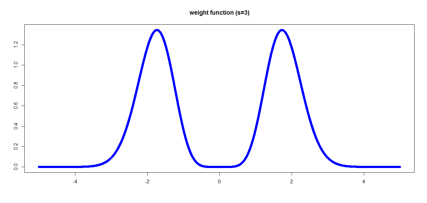
Figure 1: the weight function $w_{s}\left(x^{2}\right)$ for $s=3$.

For any resolution level $j\in\mathbb{Z}$, let $\left\{E_{jq}\right\},$ $q=1,...,Q_{j}$ be a partition of $\mathbb{S}^{1}$, such that $E_{jq_{1}}\cap E_{jq_{2}}=\varnothing$ for $q_{1}\neq q_{2}$. Any $E_{jq}$ is characterized by the couple $\left(\lambda_{jq},x_{jq}\right)$: $\lambda_{jq}=\rho\left(E_{jq}\right)$ describes the length of $E_{jq}$, while $x_{jq}\in E_{jq}$ is a point belonging to $E_{jq}$. For the sake of simplicity, we can think to $x_{jq}$ as the midpoint of the segment of arc $E_{jq}$. Fixed now the shape parameter $s\in\mathbb{N}$ and the scale parameter $B>1$, the circular Mexican needlet $\psi_{jq;s}:\mathbb{S}^{1}\mapsto\mathbb{C}$ is given by

$$\psi_{jq;s}\left(\theta\right) := \sqrt{\lambda_{jq}}\sum_{k=-\infty}^{\infty}w_{s}\left(\left(B^{-j}k\right)^{2}\right)\overline{u_{k}\left(x_{jq}\right)}u_{k}\left(\theta\right)$$ (5)

$$= \sqrt{\lambda_{jq}}\sum_{k=-\infty}^{\infty}w_{s}\left(\left(B^{-j}k\right)^{2}\right)\exp\left(ik\left(\theta-x_{jq}\right)\right)\text{, }\theta\in\mathbb{S}^{1}.$$

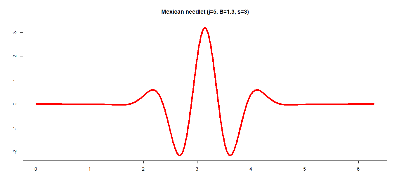
Figure 2: The Mexican Needlet with $s=3,B=1.3,j=5$ centered on the point $x_{jq}=\pi$.

For any $F\in$ $L^{2}\left(\mathbb{S}^{1}\right)$, the needlet coefficient $\beta_{jq;s}\in\mathbb{C}$ corresponding to $\psi_{jq;s}$ is given by

$$\beta_{jq;s}:=\left\langle F,\psi_{jq;s}\right\rangle_{L^{2}\left(\mathbb{S}^{1}\right)}.$$ (6)

The next result, here properly fitted for $\mathbb{S}^{1}$, was originally proposed as Theorem 1.1 in gm2 : it proves that the Mexican needlet framework describes a nearly-tight frame on the manifold. We recall that a set of functions $\left\{e_{i},i\geq 1\right\}$ defined over a manifold $M$ is a frame if there exist $c_{1},c_{2}>0$ so that, for any $F\in L^{2}\left(M\right)$,

$$c_{1}\left\|F\right\|_{L^{2}\left(M\right)}^{2}\leq\sum_{i}\left|\left\langle F,e_{i}\right\rangle_{L^{2}\left(M\right)}\right|^{2}\leq c_{2}\left\|F\right\|_{L^{2}\left(M\right)}^{2}.$$

A frame is said to be tight if $c_{1}=c_{2}$. An example of a tight frame over the $d$-dimensional sphere $\mathbb{S}^{d}$ is given by the standard needlets, introduced in the literature in npw1 ; npw2 . A frame is nearly-tight if $c_{2}/c_{1}\simeq 1+\varepsilon$, where $\varepsilon$ is close to $0$, cfr. gm1 .

Theorem 2.1

(Nearly-tightness of the Mexican needlets frame - Th. 1.1 in gm2 ) Fixing $B>1$ and $c_{0},\delta_{0}>0$ sufficiently small, there exists a constant $C_{0}$ as follows:

• for $0<\eta<1$, suppose that for each $j\in\mathbb{Z}$, there exists a set of measurable sets $\left\{E_{jq},q=1,...,Q_{j}\right\}$, with $\lambda_{jq}=\mu\left(E_{jq}\right)$, where:

  • $\lambda_{jq}\leq\eta B^{-j}$;

  • for each $j$ with $\eta B^{-j}<\delta_{0}$, $\lambda_{jq}\geq c_{0}\left(\eta B^{-j}\right)$ for $q=1,...,Q_{j}$;

• it holds that

  $$\left(\Lambda_{B,s}m_{B}\!-\!C_{0}\eta\right)\left\|F\right\|_{L^{2}\left(\mathbb{S}^{1}\right)}^{2}\!\leq\!\sum_{j=-\infty}^{\infty}\sum_{q=1}^{Q_{j}}\left|\beta_{jq;s}\right|^{2}\!\leq\!\left(\Lambda_{B,s}M_{B}\!+\!C_{0}\eta\right)\left\|F\right\|_{L^{2}\left(\mathbb{S}^{1}\right)}^{2}.$$

  If $\left(\Lambda_{B,s}m_{B}-C_{0}\eta\right)>0$, then $\left\{\psi_{jq;s}\right\}$ is a nearly tight frame, since

  $$\frac{\left(\Lambda_{B,s}M_{B}+C_{0}\eta\right)}{\left(\Lambda_{B,s}m_{B}-C_{0}\eta\right)}\sim\frac{M_{B}}{m_{B}}=1+O_{B}\left(\left|B-1\right|^{2}\log\left|B-1\right|\right).$$

Mexican needlets can be thought as an alternative approach to the standard needlets, proposed in npw1 ; npw2 , see also bkmpAoSb ; marpecbook , in views of their stronger localization property in the real domain. Standard needlets feature a quasi-exponential localization property in the spatial range, while the weight function $w_{s}$ leads to a full-exponential localization in the real space as proved below in Lemma 1 (cfr. durastanti1 ; gm2 ). As far as the frequency domain is concerned, while spherical needlets lie on compact support (see again npw1 ; npw2 ), each Mexican needlet has to take in account the whole frequency range. This issue is partially compensated by the structure itself of the function $w_{s}$, exponentially localized around a dominant term in the frequency domain and, therefore, consistently different from zero only on limited set of frequencies. For our purposes and in order to respect the conditions in Theorem 2.1, we impose the following

Condition 1

. Let $\psi_{jk;s}\left(\theta\right)$ and $\beta_{jk;s}$ be given respectively by (5) and (6). We have that, for $j>0$

$$Q_{j}\approx\eta^{-1}B^{j}\text{ , }\lambda_{jq}\approx\eta B^{-j},$$

so that

$$\psi_{jq;s}\left(\theta\right)\approx\eta^{\frac{1}{2}}B^{-\frac{j}{2}}\sum_{k=-\infty}^{\infty}w_{s}\left(\left(B^{-j}k\right)^{2}\right)\exp\left(ik\left(\theta-x_{jq}\right)\right)\text{ , }\theta\in\mathbb{S}^{1}.$$ (7)

Furthermore, we choose $J_{0}<-\log_{B}\sqrt{s}$ and fix $\delta_{0}$ such that $\delta_{0}\leq\eta B^{-J_{0}}$. Hence, we have, for $j<J_{0}$,

$$Q_{j}=1\text{, }\lambda_{jq}=2\pi.$$ (8)

Mexican needlets are characterized by the following localization property, proven in Lemma 1:

$$\left|\psi_{jk;s}\left(\theta\right)\right|\leq\!\sqrt{\lambda_{jk}}c_{s}B^{j}\exp\!\left(\!-\left(\!\frac{B^{j}\left(\theta-x_{jk}\right)}{2}\right)^{2}\right)\!\left(1+\!\left(\frac{B^{j}\left(\theta-x_{jk}\right)}{2}\right)^{2s}\right).$$

From the localization property, it follows a bound rule on the norms: there exist $\widetilde{c_{p}},\widetilde{C_{p}}>0$ such that

$$\widetilde{c_{p}}B^{j\left(\frac{p}{2}-1\right)}\eta^{\frac{p}{2}}\leq\left\|\psi_{jq;s}\right\|_{L^{p}\left(\mathbb{S}^{1}\right)}^{p}\leq\widetilde{C_{p}}\eta^{\frac{p}{2}}B^{j\left(\frac{p}{2}-1\right)}\text{ .}$$ (9)

The proof, totally analogous to the case of standard needlets (see npw2 ), is here omitted.

Remark 2

The choice of (8) is justified as follows. First of all, observe that, for any $j<J_{0}$, $\lambda_{jq}\$still satisfies Theorem 2.1. Furthermore, when $j$ is negative, the $B^{-j}$ grows to infinity, hence there exists some $J^{\prime}<0$ such that $\delta_{0}\leq\eta B^{-J^{\prime}}$. It implies that the $\lambda_{jq}$ has to be smaller than a quantity bigger  than $4\pi=\rho\left(\mathbb{S}^{1}\right)$, corresponding to the case $E_{jq}\equiv\mathbb{S}^{1}$, which leads to $Q_{j}=1$, so that we have that $Q_{j}\lambda_{jk}\approx 1$. As far as the choice of $J_{0}$ is concerned, if $J_{0}<-\log_{B}\sqrt{s}$, it means that, for any $k\,$, $\left|kB^{-J_{0}}\right|>s$, and therefore $w_{s}\left(\left(kB^{-J_{0}}\right)^{2}\right)<$ $w_{s}\left(s\right)=\max_{r\in\mathbb{R}}w_{s}\left(r\right)$. As consequence, taking into account Lemma 2, we have that for any $k$, $\chi_{s,B,J_{0}}\left(k^{2}\right)<<2^{-2s}\Gamma\left(2s\right)=e_{s}$.

Remark 3

While in gm0 ; gm1 ; gm2 ; gm3 the Mexican needlets are defined as $\psi_{j^{\prime}q}\left(\theta\right)\equiv\psi_{-jq}\left(\theta\right)$, $\theta\in\mathbb{S}^{1}$. We use this notation to uniform this work to the already existing literature on the field of statistics based on needlet-like framework.

2.2 Besov spaces on the circle

In this subsection, we will recall some of the results proposed in gm3 (see also WASA ; npw2 ) on Besov spaces, in terms of their approximation properties. More in details, let $\Pi_{r}$ be the space of polynomials of degree $r$: we start by looking for the infimum of the $L^{p}\left(\mathbb{S}^{1}\right)$-distance between a function $f:\mathbb{S}^{1}\mapsto\mathbb{R}$ and the space $\Pi_{r}$:

$$G_{r}\left(f,P\right)=\inf_{P\in\Pi_{r}}\left\|f-P\right\|_{L^{p}\left(\mathbb{S}^{1}\right)}.$$

Following, for instance, bkmpAoSb ; dgm ; gm3 ; npw2 , let $F\in\mathcal{B}_{m,t}^{r}$, if and only if both the following conditions hold:

$$\left(i\right)\text{ }F\in L^{m}\left(\mathbb{S}^{1}\right)\text{ , }\left(ii\right)\left(\sum_{u}\left(u^{s}G_{u}\left(f,P\right)\right)^{\frac{r}{u}}\right)^{\frac{1}{r}},$$

or, equivalently,

$$\left(i\right)\text{ }F\in L^{m}\left(\mathbb{S}^{1}\right)\text{ , }\left(ii\right)\left(\sum_{j}\left(B^{-jr}G_{B^{j}}\left(f,P\right)\right)^{q}\right)^{\frac{1}{q}}.$$

As shown in gm3 , see also bkmpAoSb , it holds that, for $1\leq m\leq\infty$, $r>0$, $0\leq t\leq\infty$, $f\in$ $\mathcal{B}_{m,t}^{r}$ if and only if

$$\left(\sum_{q=1}^{Q_{j}}\left|\beta_{jq;s}\right|^{m}\left\|\psi_{jk;s}\right\|_{L^{m}\left(\mathbb{S}^{1}\right)}^{m}\right)^{\frac{1}{m}}<B^{-jr}\delta_{j},\text{ }\delta_{j}\in\ell_{r}.$$

In what follows, we will make extensive use of this inequality with $m=2$:

$$\left(\sum_{q=1}^{Q_{j}}\left|\beta_{jq;s}\right|^{2}\left\|\psi_{jk;s}\right\|_{L^{2}\left(\mathbb{S}^{1}\right)}^{2}\right)^{\frac{1}{2}}\leq\left(\widetilde{C_{2}}\eta\sum_{q=1}^{Q_{j}}\left|\beta_{jq;s}\right|^{2}\right)^{\frac{1}{2}}<B^{-jr}\delta_{j},\text{ }\delta_{j}\in\ell_{r}.$$ (10)

Further details on Besov spaces can be found in npw2 and in the textbook WASA .

3 The density estimation procedure

In this section, we will introduce a thresholding density function estimator on the circle based on the Mexican needlet coefficients. As already mentioned, thresholding techniques were introduced in the literature by D. Donoho and I. Johnstone in donoho , to be later successfully applied in several research topics: for an exhaustive overview and details we suggest the textbooks WASA and tsyb . Consider a set of random directional observations $\left\{X_{i}\in\mathbb{S}^{1}:i=1,...,n\right\}$ with common distribution $v\left(\theta\right)=F\left(\theta\right)d\theta$ and let us introduce the threshold function $\zeta_{jq}\left(\tau_{n}\right):=\mathds{1}_{\left\{\left|\beta_{jq;s}\right|\geq\kappa\tau_{n}\right\}}$, where $\kappa$ is a real-valued positive constant to be chosen to set the size of the threshold (cfr. bkmpAoSb ). The coefficient estimator is given by

$$\widehat{\beta}_{jq;s}:=\frac{1}{n}\sum_{i=1}^{n}\overline{\psi}_{jq;sK}\left(X_{i}\right),$$

which is unbiased, i. e.

$$\mathbb{E}\left[\widehat{\beta}_{jqK;s}\right]=\int_{\mathbb{S}^{1}}\overline{\psi}_{jq;sK}F\left(\theta\right)d\theta=\beta_{jqK;s}.$$

Consequently, the thresholding density estimator is given by

$$\widehat{F}\left(\theta\right)=\sum_{j=J_{0}}^{J_{n}}\sum_{q=1}^{Q_{j}}\zeta_{jq}\left(\tau_{n}\right)\widehat{\beta}_{jqK;s}\psi_{jq;sK}\left(\theta\right)\text{ , }\theta\in\mathbb{S}^{1},$$ (11)

where $J_{n}$ and $K_{n}$ represent respectively the truncation resolution level and the cut-off frequency. The truncation level is chosen so that $B^{J_{n}}=\sqrt{\frac{n}{\log n}}$, as usual in the literature (see for instance bkmpAoSb ; dgm ), while the cut-off frequency is fixed so that $K_{n}=\sqrt{\frac{n}{\log n}}$, . The other tuning parameters of the Mexican needlet estimator to be considered are:

• the threshold constant $\kappa$, whose evaluation is given in the Section 6 of bkmpAoSb ;

• the scaling factor $\tau_{n}$, depending on the sample size, chosen, as usual in the literature, as $\tau_{n}=\left(\log n/n\right)^{1/2}$;

• the pixel-parameter $\eta_{n}=\eta$, chosen so that $\eta_{n}=O_{n}\left(n^{-\frac{2}{3}}\right)$.

We will present our main result concerning Mexican thresholding density estimation in the next Theorem. For the embeddings featured by the Besov spaces, as in bkmpAoSb , the condition $r>\frac{1}{m}$ implies that $F\in\mathcal{B}_{m,t}^{r}\subset\mathcal{B}_{\infty,t}^{r-\frac{1}{m}}$, so that $F$ is continuous.

Theorem 3.1

For $1\leq m=t<2$, $r>\frac{1}{m}$, there exists some constant $C_{0}=C_{0}\left(m,r\right)$ such that

$$\sup_{F\in\mathcal{B}_{m,t}^{r}}\mathbb{E}\left[\left\|\widehat{F}-F\right\|_{L^{2}\left(\mathbb{S}^{1}\right)}^{2}\right]\leq C_{0}\log n\left(\frac{n}{\log n}\right)^{-\frac{2r}{2r+1}}\text{ .}$$ (12)

Remark 4

To attain optimality, it should be necessary to show also that

$$\sup_{F\in\mathcal{B}_{m,t}^{r}}\mathbb{E}\left[\left\|\widehat{F}-F\right\|_{L^{2}\left(\mathbb{S}^{1}\right)}^{2}\right]\geq C_{*}\left(\frac{n}{\log n}\right)^{-\frac{2r}{2r+1}}.$$

This lower bound is entirely analogous to the standard needlet case in bkmpAoSb , Theorem 11, and therefore its proof is here omitted.

4 Proof of Theorem 3.1

In this section we will provide a proof for Theorem 3.1 based on the main guidelines described by D. Donoho and I. Johnstone in donoho , cfr. also bkmpAoSb and the textbooks WASA ; tsyb . The procedure illustrated by bkmpAoSb ; donoho ; donoho1 fits perfectly for tight wavelet systems, which feature an exact reconstruction formula. As already discussed in Subsection 2.1, Mexican needlet are not characterized by tightness, hence the bias term appearing in the study of (12) will also take into account addends due the (deterministic) error raising when we approximate a function with its wavelet expansion. The decay of these terms will depend on the choice of the pixel-parameter $\eta_{n},$ on one hand, and of $J_{n}$ and $K_{n}$ on the other hand. We will start by developing an upper bound for the bias term, which represents the main difference between the estimation procedure here discussed and the one based on standard needlet frames.

4.1 The bias: the construction and the upper bound

We recall from gm2 the so-called summation operator $S$, leading to the summation formula. The summation formula can be viewed as the equivalent in the Mexican needlet framework of the reconstruction formula in the standard needlet case (see for instance npw1 ; marpecbook ): for any $F\in L^{2}\left(\mathbb{S}^{1}\right)$, let the summation operator $S\left[F\right]_{s}$ be given by

$$S\left[F\right]_{s}\left(\theta\right):=\sum_{j=J_{0}}^{\infty}\sum_{q=1}^{Q_{j}}\beta_{jq;s}\psi_{jq;s}\left(\theta\right)\text{ , }\theta\in\mathbb{S}^{1}\text{.}$$ (13)

The goal of this subsection is also to estimate which terms in the sum above are so small that they can be neglected. We will fix a cut-off frequency $K$, to compensate the lack of a compact support in the harmonic domain typical of standard needlets (see npw1 ), to define the truncated Mexican needlet, and a truncation resolution level $J$. Theorem 4.1 will exploit an upper bound, depending on $s$, $J$, $K$ and $\eta$, between (13) and the truncated summation operator defined below. Observe that these results are general and not related to the specificity of the estimation problem: in this sense, when the label $n$ in $K$ and $J$ is omitted, we intend that the claimed result holds in general.
First of all, given $K\in\mathbb{N}$, the truncated Mexican needlet $\psi_{jq;sK}$ is given by

$$\psi_{jq;sK}\left(\theta\right):=\sqrt{\lambda_{jq}}\sum_{\left|k\right|\leq K}w_{s}\left(\left(kB^{-j}\right)^{2}\right)\overline{u_{k}\left(\xi_{jq}\right)}u_{k}\left(\theta\right)\text{ , }\theta\in\mathbb{S}^{1}\text{, }\xi_{jq}\in E_{jq}\text{ ,}$$

and the corresponding truncated needlet coefficient $\beta_{jq;sK}$ is defined

$$\beta_{jq;sK}:=\left\langle F,\psi_{jq;sK}\right\rangle_{L^{2}\left(\mathbb{S}^{1}\right)}\text{ .}$$

Loosely speaking, fixed $K$, $\psi_{jk;sK}\left(\cdot\right)$ is the Mexican needlet where all the elements out of the support $\left[-K,K\right]$ are not taken into account. The truncated summation operator $S\left[F\right]_{s,K,J}$ is therefore given by

$$S\left[F\right]_{s,K,J}\left(\theta\right):=\sum_{j=J_{0}}^{J}\sum_{q=1}^{Q_{j}}\beta_{jq;sK}\psi_{jq;sK}\left(\theta\right)\text{ , }\theta\in\mathbb{S}^{1}\text{.}$$ (14)

Remark 5

Following Remark 2, we will truncate in (14) all the negative resolution levels $j<J_{0}$.

Let the bias $R_{s,K,J,\eta}$ be given by

$$R_{s,K,J,\eta}:=\left\|S\left[F\right]_{s}-S\left[F\right]_{s,K,J}\right\|_{L^{2}\left(\mathbb{S}^{1}\right)}\text{ ;}$$ (15)

An upper bound for $R_{s,K,J}$ is explicitly provided in the next Theorem.

Theorem 4.1

Let $R_{s,K,J}$ be given by (15). Then, there exist $C_{1},C_{2},C_{3}>0$ such that

$$R_{s,K,J} \leq C_{1}B^{-rJ}+C_{2}J^{\frac{1}{2}}K^{2s-\frac{1}{2}}\exp\left(-K^{2}\right)B^{-\left(r+2s-\frac{1}{2}\right)J}\text{ }$$

$$+C_{3}B^{\left(1-2s\right)J}J^{\frac{1}{2}}K^{s-\frac{1}{4}}e^{-2K^{2}}\left(\sum_{\left|k\right|>K}\gamma_{k}\right)^{\frac{1}{2}}$$

Proof

Using the Minkowski inequality, we have

$$\left\|S\left[F\right]_{s}-S\left[F\right]_{s,K,J}\right\|_{L^{p}\left(\mathbb{S}^{1}\right)}\leq I_{1}+I_{2}+I_{3},$$

where

$$I_{1}:=\left\|\sum_{j=J_{0}}^{\infty}\sum_{q=1}^{Q_{j}}\beta_{jq;s}\psi_{jq;s}-\sum_{j=J_{0}}^{J}\sum_{q=1}^{Q_{j}}\beta_{jq;s}\psi_{jq;s}\right\|_{L^{2}\left(\mathbb{S}^{1}\right)};$$

$$I_{2}:=\left\|\sum_{j=J_{0}}^{J}\sum_{q=1}^{Q_{j}}\beta_{jq;s}\psi_{jq;s}-\sum_{j=J_{0}}^{J}\sum_{q=1}^{Q_{j}}\beta_{jq;s}\psi_{jq;s,K}\right\|_{L^{2}\left(\mathbb{S}^{1}\right)};$$

$$I_{3}:=\left\|\sum_{j=J_{0}}^{J}\sum_{q=1}^{Q_{j}}\beta_{jq;s}\psi_{jq;sK}-\sum_{j=J_{0}}^{J}\sum_{q=1}^{Q_{j}}\beta_{jq;sK}\psi_{jq;sK}\right\|_{L^{2}\left(\mathbb{S}^{1}\right)}.$$

Observe that while $I_{1}$ describes the bias due to the truncation of the resolution levels belonging to $\left(J,\infty\right)$, $I_{2}$ and $I_{3}$ depend strictly on the choice of the cut-off frequency $K$, due to the approximation error due to approximate Mexican needlets by the corresponding truncated ones (the former), and Mexican needlet coefficients by the corresponding truncated ones (the latter). According to Lemma 6, we get

$$I_{1}\leq C_{1,1}B^{-rJ}\text{.}$$

As far as $I_{2}$ is concerned, from Lemma 7, we obtain

$$I_{2}\leq C_{2}J^{\frac{1}{2}}K^{2s-\frac{1}{2}}\exp\left(-K^{2}\right)B^{-\left(r+2s-\frac{1}{2}\right)J}\text{ .}$$

Finally, from Lemma 8, it holds that

$$I_{3}\leq C_{3}B^{\left(1-2s\right)J}J^{\frac{1}{2}}K^{s-\frac{1}{4}}e^{-2K^{2}}\left(\sum_{\left|k\right|>K}\gamma_{k}\right)^{\frac{1}{2}}\text{ ,}$$

as claimed.

Remark 6

An analogous result is obtained in Theorem 2.5 in gm2 (see also Lemma 2.3 in gm1 ). In these works, the authors use a generic weight function belonging to the Schwarz space and, moreover, the wavelets studied are defined over a general compact manifold. For this reason, the bound exploited in Theorem 4.1, using explicit bounds provided by $w_{s}$ and by the basis $\left\{u_{k}\right\}$, is more precise.

4.2 Adaptivity of $\widehat{F}$ for the $L^{2}$-risk

Merging the results achieved in the previous subsection with the ones driven by the standard procedure in the case of nonparametric thresholding density estimation (see for instance bkmpAoSb ), we obtain the following proof.

Proof (Proof ot the Theorem 3.1)

Observe that, for the triangular inequality, we have

$$\mathbb{E}\!\left[\!\left\|\widehat{F}-F\right\|_{L^{2}\left(\mathbb{S}^{1}\right)}^{2}\!\right]\! =\!\mathbb{E}\left[\left\|\widehat{F}-S\left[F\right]_{s,K_{n},J_{n}}+S\left[F\right]_{s,K_{n},J_{n}}-S\left[F\right]_{s}+S\left[F\right]_{s}-F\right\|_{L^{2}\left(\mathbb{S}^{1}\right)}^{2}\right]$$

$$\leq E_{1}+E_{2}+E_{3}\text{ ,}$$

where

$$E_{1} = \mathbb{E}\left[\left\|\widehat{F}-S\left[F\right]_{s,K_{n},J_{n}}\right\|_{L^{2}\left(\mathbb{S}^{1}\right)}^{2}\right]\text{ ;}$$

$$E_{2} = R_{s,K_{n},J_{n}}^{2}\text{ ;}$$

$$E_{3} = \left\|S\left[F\right]_{s}-F\right\|_{L^{2}\left(\mathbb{S}^{1}\right)}^{2}\text{ .}$$

As far as $E_{1}$ is concerned, the bound is established analogously to the one achieved in bkmpAoSb , hence here it is given just a sketch of this proof in Lemma 9 (see also dgm ). Indeed, we have:

$$E_{1} = \mathbb{E}\left[\left\|\sum_{j=0}^{J_{n}}\sum_{q=1}^{Q_{j}}\left(\zeta_{jq}\left(\tau_{n}\right)\widehat{\beta}_{jq;sK_{n}}-\beta_{jq;sK_{n}}\right)\psi_{jq;sK_{n}}\right\|_{L^{2}\left(\mathbb{S}^{1}\right)}^{2}\right]$$

$$\leq \left(J_{n}+1\right)\sum_{j=0}^{J_{n}}\mathbb{E}\left[\left\|\sum_{q=1}^{Q_{j}}\left(\zeta_{jq}\left(\tau_{n}\right)\widehat{\beta}_{jq;sK_{n}}-\beta_{jq;sK_{n}}\right)\psi_{jq;sK_{n}}\right\|_{L^{2}\left(\mathbb{S}^{1}\right)}^{2}\right]$$

$$\leq \left(J_{n}+1\right)\sum_{j=0}^{J_{n}}\sum_{q=1}^{Q_{j}}\left\|\psi_{jq;sK_{n}}\right\|_{L^{2}\left(\mathbb{S}^{1}\right)}^{2}\mathbb{E}\left[\left|\zeta_{jq}\left(\tau_{n}\right)\widehat{\beta}_{jq;sK_{n}}-\beta_{jq;sK_{n}}\right|^{2}\right]$$

$$\leq \left(J_{n}+1\right)\widetilde{C_{2}}\eta_{n}\sum_{j=0}^{J_{n}}\sum_{q=1}^{Q_{j}}\mathbb{E}\left[\left|\zeta_{jq}\left(\tau_{n}\right)\widehat{\beta}_{jq;sK_{n}}-\beta_{jq;sK_{n}}\right|^{2}\right]$$

$$\leq C_{1}J_{n}\left(E_{1,1}+E_{1,2}+E_{1,3}+E_{1,4}\right)\text{ ,}$$

where

$$E_{1,1}= \eta_{n}\sum_{j=0}^{J_{n}}\sum_{q=1}^{Q_{j}}\mathbb{E}\left[\left|\zeta_{jq}\left(\tau_{n}\right)\widehat{\beta}_{jq;sK_{n}}-\beta_{jq;sK_{n}}\right|^{2}\mathds{1}_{\left\{\left|\widehat{\beta}_{jq;sK_{n}}\right|\geq\kappa\tau_{n}\right\}}\mathds{1}_{\left\{\left|\beta_{jq;sK_{n}}\right|\geq\frac{\kappa\tau_{n}}{2}\right\}}\right];$$ (16)

$$E_{1,2}= \eta_{n}\sum_{j=0}^{J_{n}}\sum_{q=1}^{Q_{j}}\mathbb{E}\left[\left|\zeta_{jq}\left(\tau_{n}\right)\widehat{\beta}_{jq;sK_{n}}-\beta_{jq;sK_{n}}\right|^{2}\mathds{1}_{\left\{\left|\widehat{\beta}_{jq;sK_{n}}\right|\geq\kappa\tau_{n}\right\}}\mathds{1}_{\left\{\left|\beta_{jq;sK_{n}}\right|\leq\frac{\kappa\tau_{n}}{2}\right\}}\right];$$ (17)

$$E_{1,3}= \eta_{n}\sum_{j=0}^{J_{n}}\sum_{q=1}^{Q_{j}}\left|\beta_{jq;sK_{n}}\right|^{2}\mathbb{E}\left[\mathds{1}_{\left\{\left|\widehat{\beta}_{jq;sK_{n}}\right|<\kappa\tau_{n}\right\}}\mathds{1}_{\left\{\left|\beta_{jq;sK_{n}}\right|\geq 2\kappa\tau_{n}\right\}}\right];$$ (18)

$$E_{1,4}= \eta_{n}\sum_{j=0}^{J_{n}}\sum_{q=1}^{Q_{j}}\left|\beta_{jq;sK_{n}}\right|^{2}\mathbb{E}\left[\mathds{1}_{\left\{\left|\widehat{\beta}_{jq;sK_{n}}\right|<\kappa\tau_{n}\right\}}\mathds{1}_{\left\{\left|\beta_{jq;sK_{n}}\right|<2\kappa\tau_{n}\right\}}\right].$$ (19)

Heuristically, the cross-terms $E_{1,2}$ and $E_{1,3}$ are bounded by means of fast decays of the probabilistic inequalities given in Lemma 10, while as far as $E_{1,1}$ and $E_{1,4}$ are concerned, their bounds will be exploited according to the tail properties of the Besov spaces: further details are in Lemma 9. From these considerations, it follows that

$$E_{1}\leq C_{1}\left(\frac{n}{\log n}\right)^{-\frac{2r}{2r+1}}.$$

As far as $E_{2}$ is concerned, from Theorem 4.1, it holds that

$$E_{2}= \leq C_{1}B^{-rJ_{n}}+C_{2}J^{\frac{1}{2}}K_{n}^{2s-\frac{1}{2}}\exp\left(-K_{n}^{2}\right)B^{-\left(r+2s-\frac{1}{2}\right)J_{n}}$$

$$+C_{3}B^{\left(1-2s\right)J_{n}}J_{n}^{\frac{1}{2}}K_{n}^{s-\frac{1}{4}}\exp\left({-2K_{n}^{2}}\right)\left(\sum_{\left|k\right|>K_{n}}\gamma_{k}\right)^{\frac{1}{2}}$$

Observe that

$$B^{-2rJ_{n}}=\left(\frac{n}{\log n}\right)^{-r}\leq\left(\frac{n}{\log n}\right)^{-\frac{2r}{2r+1}}\text{ ,}$$

while

$$C_{2}J_{n}^{\frac{1}{2}}K_{n}^{2s-\frac{1}{2}}\exp\left(-K_{n}^{2}\right)B^{-\left(r+2s-\frac{1}{2}\right)J_{n}}\leq\frac{n}{\log n}^{-\frac{2r}{2r+1}}$$

$$B^{\left(1-2s\right)J_{n}}J_{n}^{\frac{1}{2}}K_{n}^{s-\frac{1}{4}}e^{-2K_{n}^{2}}\leq\frac{n}{\log n}^{-\frac{2r}{2r+1}}$$

Finally, we have

$$\left\|S\left[F\right]_{s}-F\right\|_{L^{2}\left(\mathbb{S}^{1}\right)}^{2}\leq C_{3}\eta_{n}\text{ ,}$$

whence, for $r>1$,

$$\eta_{n}\leq n^{-\frac{3}{4}}\leq\frac{n}{\log n}^{-\frac{3}{4}}\leq\frac{n}{\log n}^{-\frac{2r}{2r+1}}\text{ .}$$

5 Numerical results

This section presents the results of some numerical experiments. Obviously, in the framework of finite sample situation, the asymptotic rate given in Theorem 3.1 has to be considered just as a prompt. In what follows, we have built an estimator (11) using the set to estimate $F\left(\theta\right)=\left(2\pi\right)^{-1}\exp\left(\left(\theta-\pi\right)^{2}/2\right)$ by using CRAN R. Some graphical evidence can be found in Figure 3. We will focus on two main points:

• the number of coefficients surviving to the thresholding procedure depending on $\kappa$ and $\tau_{n}$.

• the estimate of the $L^{2}$-risk function $\left\|\widehat{F}-F\right\|_{L^{2}\left(\mathbb{S}^{1}\right)}$ depending on the number of observations $n$.

In particular, following bkmpAoSb , we have chosen $\kappa=\kappa_{0}\sqrt{0.107}\sup_{\theta\in\mathbb{S}^{1}}\left|F\left(\theta\right)\right|$, with $\kappa_{0}=0.05,0.1,0.15,0.2$, and $n=8000,12000$, leading to $K_{8000}=30$, $K_{12000}=36$, $J_{8000}=10$, $J_{12000}=11$, $t_{8000}=0.0335$ and $t_{12000}=0.028$. The Table 1 counts the number of coefficients survived to thresholding. A qualitative analysis confirms that: (i) as $n\rightarrow\infty$, $t_{n}$ is decreasing so that the threshold is lower and more $\widehat{\beta}_{jq;s}$ survive to the thresholding procedure and (ii) if $\kappa_{0}$ increases, the number of surviving coefficients is smaller, expecially at higher resolution levels.
The Table 2 describes the estimates of the $L^{2}$-risks for any choice of $\kappa_{0}$ and any $n$. As expected, the $L^{2}$-risk    is decreasing when $n$ grows and it is increasing with respect to $\kappa_{0}$ (cfr. bkmpAoSb )

	n=8000			n=12000
$j\backslash\kappa_{0}$	0.10	0.15	0.20	0.10	0.15	0.20	Tot
0	1	1	1	1	1	1	1
1	1	1	1	1	1	1	1
2	2	2	2	2	2	2	2
3	3	3	3	3	3	2	3
4	4	4	4	4	3	3	4
5	5	4	4	5	5	5	5
6	8	7	6	8	7	6	8
7	11	10	10	10	10	9	11
8	13	11	11	13	14	14	15
9	19	14	12	20	21	18	21
10	17	4	3	28	12	10	29
11	NA	NA	NA	7	2	0	40

Table 1: number of mexican needlet coefficients surviving thresholding for various values of $n$, $j$ and $\kappa_{0}$.

	n=8000			n=12000
$\kappa_{0}$	0.10	0.15	0.20	0.10	0.15	0.20
$L^{2}$-risk	0.481	0.468	0.451	0.458	0.432	0.331

Table 2: $L^{2}$-risk for various values of $n$ and $\kappa_{0}$.

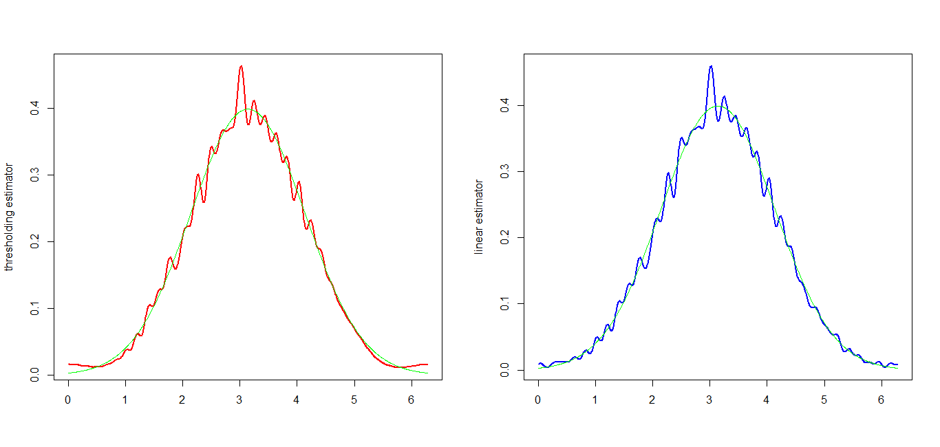
Figure 3: Graphs of the thresholding estimator (on the left) and of the linear (not-thresholded) estimator (on the right) for $n=12000$ and $s=3$.

6 Auxiliary results

This section contains all the statements and the proofs of the auxiliary results used to prove Theorem 3.1 and Theorem 4.1.

6.1 Properties and Inequalities for Mexican needlets

The first result here presented concerns the concentration property of the Mexican needlets in the real domain.

Lemma 1

For every $\theta\in\mathbb{S}^{1},$ $s\geq 1$, there exists $c_{s}$ such that:

$$\left|\psi_{jq;s}\left(\theta\right)\right|\!\leq\!\sqrt{\lambda_{jq}}c_{s}B^{j}\exp\!\left(\!-\left(\frac{B^{j}\left(\theta-x_{jq}\right)}{2}\right)^{2}\right)\!\left(\!1+\left(\frac{B^{j}\left(\theta-x_{jq}\right)}{2}\right)^{2s}\right).$$

Furthermore, if $j\geq 0$, it holds that

$$\left|\psi_{jq;s}\left(\theta\right)\right|\leq c_{s}\eta B^{\frac{j}{2}}\exp\left(-\left(\frac{B^{j}\left(\theta-x_{jq}\right)}{2}\right)^{2}\right)\left(1+\left(\frac{B^{j}\left(\theta-x_{jq}\right)}{2}\right)^{2s}\right).$$

Proof

This proof follows strictly the one for standard needlets developed in npw1 and the one for Mexican needlets on $\mathbb{S}^{2}$ in durastanti1 , see also marpecbook . First of all, from (4) observe that we can define a function $W_{s}:\mathbb{R}\mapsto\mathbb{R}_{+}$ such that $W_{s}\left(x\right)=w_{s}\left(x^{2}\right)$. We can therefore rewrite (5) as follows:

$$\psi_{jq;s}\left(\theta\right)=\sqrt{\lambda_{jq}}\sum_{k=-\infty}^{\infty}g_{B^{j},\theta-x_{jq}}\left(k\right),$$

where

$$g_{B^{j},\theta,x_{jq}}\left(u\right):=W_{s}\left(uB^{-j}\right)\exp\left(iu\left(\theta-x_{jq}\right)\right).$$

For the Poisson summation formula (see for instance npw1 ; durastanti1 ; marpecbook ), we have that

$$\sum_{k=-\infty}^{\infty}g_{B^{j},\theta,x_{jq}}\left(k\right)=\sum_{\nu=-\infty}^{\infty}\mathcal{F}\left[g_{B^{j},\theta,x_{jq}}\right]\left(2\pi\nu\right),$$

where the symbol $\mathcal{F}\left[g\right]$ denotes the Fourier transform of $g$. In our case, we have

$$\mathcal{F}\left[g_{B^{j},\theta x_{jq}}\right]\left(\omega\right)=\mathcal{F}\left[W_{s}\left(uB^{-j}\right)\right]\ast\mathcal{F}\left[\exp\left(iu\left(\theta-x_{jq}\right)\right)\right],$$

where the symbol $\ast$ denotes the convolution product. Standard calculations lead to

$$\mathcal{F}\left[W_{s}\left(uB^{-j}\right)\right]=\frac{\left(-1\right)^{s}}{\sqrt{2}B^{-j}}H_{2s}\left(\frac{\omega}{2B^{-j}}\right)\exp\left(-\left(\frac{\omega}{2B^{-j}}\right)^{2}\right);$$

$$\mathcal{F}\left[\exp\left(iu\left(\theta-x_{jq}\right)\right)\right]=\sqrt{2\pi}\delta\left(\left(\theta-x_{jq}\right)-\omega\right).$$

Hence we get

$$\mathcal{F}\left[g_{B^{j},\theta,x_{jq}}\right]\left(\omega\right)=\frac{\left(-1\right)^{s}\sqrt{\pi}}{B^{-j}}H_{2s}\left(\frac{\left(\theta-x_{jq}\right)-\omega}{2B^{-j}}\right)\exp\left(-\left(\frac{\left(\theta-x_{jq}\right)-\omega}{2B^{-j}}\right)^{2}\right).$$

Following Proposition 2 in durastanti1 , we have that

$$\sum_{\nu=-\infty}^{\infty}\mathcal{F}\left[\widehat{g}_{B^{j},\theta-x_{jq}}\right]\left(2\pi\nu\right)\leq C_{2s}B^{j}\exp\left(-\left(\frac{B^{j}\left(\theta-x_{jq}\right)}{2}\right)^{2}\right)H_{2s}\left(\frac{B^{j}\left(\theta-x_{jq}\right)}{2}\right).$$

It can be easily proved that

$$H_{2s}\left(\frac{B^{j}\left(\theta-x_{jq}\right)}{2}\right)\approx\left(1+\left(\frac{B^{j}\left(\theta-x_{jq}\right)}{2}\right)^{2s}\right),$$

see for instance durastanti2 . Straightforward calculations lead to the claimed result.

The next results will be pivotal to truncate negative resolution levels and the frequencies $k:\left|k\right|>K$ in the summation formula.

Lemma 2

Let $w_{s}:\mathbb{R}\mapsto\mathbb{R}_{+}$ be given by (4). Let $J_{0}\in\mathbb{N}$. Hence, for $t>0$, it holds that

$$\sum_{j=-\infty}^{-J_{0}}\left|w_{s}\left(tB^{-2j}\right)\right|^{2}=\frac{\chi_{s,B,J_{0}}\left(t\right)}{2\log B}\left(1\pm O\left(\left|B-1\right|^{2}\log\left|B-1\right|\right)\right),$$ (20)

where

$$\chi_{s,B,J_{0}}\left(t\right):=2^{-2s}\Gamma\left(2s,2tB^{\frac{J_{0}}{\log B}}\right).$$

Furthermore, it holds that

$$\sum_{j=J_{0}}^{\infty}\left|w_{s}\left(tB^{-2j}\right)\right|^{2}=\frac{\phi_{s,B,J_{0}}\left(t\right)}{2\log B}\left(1\pm O\left(\left|B-1\right|^{2}\log\left|B-1\right|\right)\right),$$ (21)

where

$$\phi_{s,B,J_{0}}\left(t\right):=2^{-2s}\gamma\left(2s,2tB^{\frac{J_{0}}{\log B}}\right).$$

Proof

Let us start by proving (20). First of all, observe that the following identity holds:

$$\int_{B^{\frac{J_{0}}{\log B}}}^{\infty}\left|w_{s}\left(tx\right)\right|^{2}\frac{dx}{x}=2^{-2s}\Gamma\left(2s,2tB^{\frac{J_{0}}{\log B}}\right)=\chi_{s,B,J_{0}}\left(t\right).$$

Applying an analogous procedure to the one adopted in Lemma 7.6 in gm0 , define the function $G_{s}:\mathbb{R}\mapsto\mathbb{R}_{+}$ by

$$G_{s}\left(u\right):=\left|w_{s}\left(e^{u}\right)\right|^{2}=e^{-2e^{u}\left(1-sue^{-u}\right)}.$$

Let $j^{\prime}=-j$, and fix $t=e^{v}$, $v>0$; on one hand we get

$$\sum_{j^{\prime}=J_{0}}^{\infty}\left|w_{s}\left(tB^{2j^{\prime}}\right)\right|^{2}=\sum_{j^{\prime}=J_{0}}^{\infty}\left|w_{s}\left(e^{dj^{\prime}+v}\right)\right|^{2}=\sum_{j^{\prime}=J_{0}}^{\infty}G_{s}\left(dj^{\prime}+v\right),$$

$d=2\log B$. On the other hand, for $u=\log x$, we obtain

$$\int_{B^{\frac{J_{0}}{\log B}}}^{\infty}\left|w_{s}\left(tx\right)\right|^{2}\frac{dx}{x}=\int_{J_{0}}^{\infty}\left|w_{s}\left(e^{u+v}\right)\right|^{2}du=\int_{J_{0}}^{\infty}G_{s}\left(u+v\right)du.$$

As in Lemma 7.6 in gm0 , note that $d\sum_{j^{\prime}=J_{0}}^{\infty}G_{s}\left(dj^{\prime}+v\right)$ is a Riemann sum for $\int_{B^{\frac{J_{0}}{\log B}}}^{\infty}G_{s}\left(u+v\right)du$. Moreover, because $\sum_{j^{\prime}=J_{0}}^{\infty}G_{s}\left(dj^{\prime}+v\right)$ is periodic with period $d$, it is sufficient to estimate this sum just for $0<v<d$. Now observe that, for $J=J_{0}+\Delta J$, $\Delta J>0$, we get

$$\left|d\sum_{j^{\prime}=J_{0}}^{\infty}G_{s}\left(dj^{\prime}+v\right)-\chi_{s,B,J_{0}}\left(t\right)\right|= \left|d\sum_{j^{\prime}=J_{0}}^{\infty}G_{s}\left(dj^{\prime}+v\right)-\int_{J_{0}}^{\infty}G_{s}\left(u+v\right)du\right|$$

$$\leq \left|d\!\sum_{j^{\prime}=J_{0}}^{J}\!G_{s}\!\left(dj^{\prime}+v\right)\!-\!\int_{J_{0}}^{Jd+\frac{d}{2}}\!G_{s}\!\left(u+v\right)\!du\right|$$

$$+ d\sum_{j^{\prime}>J}G_{s}\left(dj^{\prime}+v\right)\!+\!\int_{Jd+\frac{d}{2}}^{\infty}G_{s}\left(u+v\right)du.$$

Using the midpoint rule, (see again Lemma 7.6 in gm0 ), we obtain

$$\left|d\sum_{j^{\prime}=J_{0}}^{J}G_{s}\left(dj^{\prime}+v\right)-\int_{J_{0}}^{Jd+\frac{d}{2}}G_{s}\left(u+v\right)du\right|\leq\frac{1}{24}\left\|G^{\prime\prime}\right\|_{\infty}\left(J-J_{0}\right)d^{3}.$$

On the other hand, observe that, for $r>0$,

$$\frac{d}{dr}\left(1-sre^{-r}\right)=se^{-r}\left(r-1\right),$$

so that $\left(1-sre^{-r}\right)$ is monotonically decreasing for $r\in\left[0,1\right)$, it attains its minimum for $r=1$ and then it is monotonically increasing for $r\in\left(1,\infty\right)$. Observing that $\left(1-sre^{-r}\right)_{r=0}=1$ and $\lim_{r\rightarrow\infty}\left(1-sre^{-r}\right)=1$ yields to

$$G_{s}\left(r\right)\leq e^{-2e^{r}\left(1-sre^{-r}\right)}\leq e^{-2e^{r}}.$$

Consequently, for $j^{\prime\prime}=\exp dj^{\prime}$, we obtain

$$d\sum_{j^{\prime}>J}G_{s}\left(dj^{\prime}+v\right)\leq\sum_{j^{\prime}>J}e^{-2e^{dj^{\prime}+v}}=\sum_{j^{\prime\prime}>\exp dJ}e^{-2e^{v}j^{\prime\prime}}=\frac{e^{2e^{v}\left(1-e^{dJ}\right)}}{e^{2e^{v}}-1},$$

which, for $y=2e^{u+v}$, leads to

$$\int_{Jd+\frac{d}{2}}^{\infty}G_{s}\left(u+v\right)du = \int_{Jd+\frac{d}{2}}^{\infty}e^{-2e^{u+v}}du$$

$$= \int_{2e^{Jd+\frac{d}{2}+v}}^{\infty}e^{-y}\frac{dy}{y}$$

$$\leq 2e^{-\left(Jd+\frac{d}{2}+v\right)}e^{-2e^{Jd+\frac{d}{2}+v}}.$$

Therefore, there exists a constant $C>0$ so that

$$\left|\sum_{j^{\prime}=J_{0}}^{\infty}G_{s}\left(dj^{\prime}+v\right)-\frac{\chi_{s,B,J_{0}}\left(t\right)}{d}\right| \leq \frac{1}{24}\left\|G^{\prime\prime}\right\|_{\infty}\Delta Jd^{2}+\frac{e^{2e^{v}\left(1-e^{dJ}\right)}}{e^{2e^{v}}-1}$$

$$+2e^{-\left(Jd+\frac{d}{2}+v\right)}e^{-2e^{Jd+\frac{d}{2}+v}}$$

$$\leq C\left(\Delta Jd^{2}+e^{-2e^{Jd}}\right)\leq C^{\prime}\Delta Jd^{2}.$$

According again to gm0 , we choose $\Delta J\in\left(\log\left(1/d\right)/d,2\log\left(1/d\right)/d\right)$ so that

$$\left|\sum_{j=-\infty}^{-J_{0}}\left|w_{s}\left(tB^{-2j}\right)\right|^{2}-\frac{\chi_{s,B,J_{0}}\left(t\right)}{d}\right|\leq C^{\prime}\left(2d\log\left(\frac{1}{d}\right)\right).$$

It follows that

$$\left|\left(\frac{\chi_{s,B,J_{0}}\left(t\right)}{d}\right)^{-1}\sum_{j=-\infty}^{-J_{0}}\left|w_{s}\left(tB^{-2j}\right)\right|^{2}-1\right|\leq 2\frac{C^{\prime}}{\chi_{s,B,J_{0}}\left(t\right)}d^{2}\log\left(\frac{1}{d}\right).$$

Finally, because $d=2\log B$ and $\lim_{B\rightarrow 1^{+}}\log B/\left(B-1\right)=1$, the proof is complete. The proof of (21) is totally analogous and, therefore, omitted.

Lemma 3

Let $w_{s}:\mathbb{R}\mapsto\mathbb{R}_{+}$ be given by (4). Then we have

$$\sum_{\left|k\right|>K}w_{s}^{2}\left(\left(kB^{-j}\right)^{2}\right)\leq 2^{-\left(2s+\frac{1}{2}\right)}B^{j}\Gamma\left(2s+\frac{1}{2},2K^{2}B^{-2j}\right).$$

Proof

Observe that

$$\sum_{\left|k\right|>K}w_{s}^{2}\left(\left(kB^{-j}\right)^{2}\right) = \sum_{\left|k\right|>K}\left(B^{-j}k\right)^{4s}\exp\left(-2\left(B^{-j}k\right)^{2}\right)$$

$$\leq 2\int_{K}^{\infty}\left(B^{-j}x\right)^{4s}\exp\left(-2\left(B^{-j}x\right)^{2}\right)dx$$

$$\leq 2^{-\left(2s+\frac{1}{2}\right)}B^{j}\left(\int_{2K^{2}B^{-2j}}^{\infty}u^{2s-\frac{1}{2}}\exp\left(-u\right)du\right)$$

$$\leq 2^{-\left(2s+\frac{1}{2}\right)}B^{j}\Gamma\left(2s+\frac{1}{2},2K^{2}B^{2-j}\right),$$

as claimed.

Corollary 1

Let $\omega,J>0$; for $x$ sufficiently large, it holds that

$$\sum_{j=J_{0}}^{J}B^{-\omega j}\Gamma\left(S+1,xB^{-2j}\right)\leq C_{S,\alpha}x^{S}e^{-x}B^{-\left(\omega+2S\right)J}.$$

Proof

For $x$ sufficiently large, the following limit holds

$$\lim_{x\rightarrow\infty}\frac{\Gamma\left(S+1,xB^{-2j}\right)}{\left(xB^{-2j^{\prime}}\right)^{S}e^{-xB^{-2j}}}=1,$$

see for instance abramovitzstegun Formula 6.5.32, pag. 263. Therefore, we have:

$$\sum_{j=0}^{J}B^{-\left(\omega+2S\right)j}x^{S}e^{-xB^{-2j}}\leq x^{S}e^{-x}\sum_{j=0}^{J}B^{-\left(\omega+2S\right)j}\leq C_{S,\omega}x^{S}e^{-x}B^{-\left(\omega+2S\right)J}.$$

The next result concerns the behaviour of the sums of the powers of the weights $\lambda_{jq}$.

Lemma 4

Let $Q_{j}$ and $\lambda_{jq}$ be so that Theorem 2.1 holds. For any $j$, it holds that

$$\sum_{q=1}^{Q_{j}}\lambda_{jq}\approx 1.$$

Furthermore, let $p>1$ and $j>0$. It holds that

$$\sum_{q=1}^{Q_{j}}\lambda_{jq}^{p}\leq\eta^{p-1}B^{j\left(1-p\right)}.$$ (22)

Proof

The first inequality follows directly the conditions in Theorem 2.1. On the other hand, for $j>0$, it is immediate to see that

$$\sum_{q=1}^{Q_{j}}\lambda_{jq}^{p}\leq\eta^{p}\sum_{q=1}^{Q_{j}}B^{-jp}\leq\eta^{p}Q_{j}B^{-jp}\leq\eta^{p-1}B^{j\left(1-p\right)}.$$

The next Lemma establishes explicit upper bounds for the sums with respect to $q$ of differences between Mexican standard and truncated coefficients and for the $L^{2}$-norms of the sums with respect to $q$ of Mexican standard and truncated needlets.

Lemma 5

For $j>0$, it holds that

$$\sum_{q=1}^{Q_{j}}\left|\beta_{jq;sK}-\beta_{jq;s}\right|^{2}\leq B^{j}\Gamma\left(2s+\frac{1}{2},2K^{2}B^{-2j}\right)\sum_{\left|k\right|>K}\gamma_{k}\text{ ;}$$ (23)

$$\left\|\left(\psi_{jq;sK}-\psi_{jq;s}\right)\right\|_{L^{2}\left(\mathbb{S}^{1}\right)}^{2}\leq 2^{-\left(2s+\frac{1}{2}\right)}\eta\Gamma\left(2s+\frac{1}{2},2K^{2}B^{-2j}\right)\text{ .}$$ (24)

Proof

For the Hölder inequality, it holds that

$$\sum_{q=1}^{Q_{j}}\left|\beta_{jq;sK}-\beta_{jq;s}\right|^{2} = \sum_{q=1}^{Q_{j}}\lambda_{jq}\left|\sum_{\left|k\right|>K}w_{s}\left(\left(kB^{-j}\right)^{2}\right)a_{k}u_{k}\left(\xi_{jq}\right)\right|^{2}$$

$$\leq \sum_{q=1}^{Q_{j}}\lambda_{jq}\left(\sum_{\left|k\right|>K}w_{s}\left(\left(kB^{-j}\right)^{2}\right)\left|a_{k}\right|\left|u_{k}\left(\xi_{jq}\right)\right|\right)^{2}$$

$$\leq \sum_{q=1}^{Q_{j}}\lambda_{jq}\sum_{\left|k\right|>K}w_{s}^{2}\left(\left(kB^{-j}\right)^{2}\right)\sum_{\left|k\right|>K}\left|a_{k}\right|^{2}\left|u_{k}\left(\xi_{jq}\right)\right|^{2}$$

$$\leq \sum_{q=1}^{Q_{j}}\lambda_{jq}\sum_{\left|k\right|>K}w_{s}^{2}\left(\left(kB^{-j}\right)^{2}\right)\sum_{\left|k\right|>K}\gamma_{k}.$$

Using Lemma 3 and Lemma 4 leads to the claimed result. As far as (24) is concerned, we get

$$\left(\psi_{jq;sK}\left(\theta\right)-\psi_{jq;s}\left(\theta\right)\right)^{2} = \lambda_{jq}\left(\sum_{\left|k\right|>K}w_{s}\left(\left(kB^{-j}\right)^{2}\right)\overline{u_{k}\left(\xi_{jq}\right)}u_{k}\left(\theta\right)\right)^{2}$$

$$= \int_{\mathbb{S}^{1}}\lambda_{jq}\left(\sum_{\left|k_{1}\right|,\left|k_{2}\right|>K}w_{s}^{2}\left(\left(kB^{-j}\right)^{2}\right)\right).$$

Using the orthogonality of $\left\{u_{k}\right\}$ and Lemma 3 yields to

$$\left\|\left(\psi_{jq;sK}-\psi_{jq;s}\right)\right\|_{L^{2}\left(\mathbb{S}^{1}\right)}^{2} = \int_{\mathbb{S}^{1}}\lambda_{jq}\left(\sum_{\left|k_{1}\right|,\left|k_{2}\right|>K}w_{s}^{2}\left(\left(kB^{-j}\right)^{2}\right)\right)$$

$$\leq 2^{-\left(2s+\frac{1}{2}\right)}\eta\Gamma\left(2s+\frac{1}{2},2K^{2}B^{-2j}\right),$$

as claimed.

6.2 Ancillary results related to Theorem 4.1

The lemmas here proved describe the behaviour of $I_{1}$, $I_{2}$ and $I_{3}$. Hence, they are pivotal to study the bias $R_{s,K,J,\eta}$.

Lemma 6

Let $I_{1}$ be given by

$$I_{1}:=\left\|\sum_{j>J}\sum_{q=1}^{Q_{j}}\beta_{jq;s}\psi_{jq;s}\right\|_{L^{2}\left(\mathbb{S}^{1}\right)}.$$

Then, there exists $C_{1}>0$ such that

$$I_{1}\leq C_{1}B^{-rJ}.$$

Proof

Note preliminarily that

$$I_{1}\leq\sum_{j>J}\left\|\sum_{q=1}^{Q_{j}}\beta_{jq;s}\psi_{jq;s}\right\|_{L^{2}\left(\mathbb{S}^{1}\right)}.$$

Observe that, for the Hölder inequality (see also bkmpAoSb ), we get

$$\left(\sum_{q=1}^{Q_{j}}\left|\beta_{jq;s}\psi_{jq;s}\left(\theta\right)\right|\right)^{2} = \left(\sum_{q=1}^{Q_{j}}\left|\beta_{jq;s}\right|\left|\psi_{jq;s}\left(\theta\right)\right|^{\frac{1}{2}}\left|\psi_{jq;s}\left(\theta\right)\right|^{\frac{1}{2}}\right)^{2}$$

$$\leq \left(\sum_{q=1}^{Q_{j}}\left|\beta_{jq;s}\right|^{2}\left|\psi_{jq;s}\left(\theta\right)\right|\right)\left(\sum_{q=1}^{Q_{j}}\left|\psi_{jq;s}\left(\theta\right)\right|\right)$$

$$\leq C\eta^{\frac{1}{2}}B^{\frac{j}{2}}\sum_{q=1}^{Q_{j}}\left|\beta_{jq;s}\right|^{2}\left|\psi_{jq;s}\left(\theta\right)\right|.$$

For $C>0$ and using (10), it follows that

$$\left\|\sum_{q=1}^{Q_{j}}\beta_{jq;s}\psi_{jq;s}\right\|_{L^{2}\left(\mathbb{S}^{1}\right)}^{2} \leq C\eta^{\frac{1}{2}}B^{\frac{j}{2}}\sum_{q=1}^{Q_{j}}\left|\beta_{jq;s}\right|^{2}\left\|\psi_{jq;s}\right\|_{L^{1}\left(\mathbb{S}^{1}\right)}$$

$$\leq C\sum_{q=1}^{Q_{j}}\eta\left|\beta_{jq;s}\right|^{2}\leq CB^{-2rj}.$$

Hence, we obtain

$$I_{1,1}=\sum_{j>J}\left\|\sum_{q=1}^{Q_{j}}\beta_{jq;s}\psi_{jq;s}\right\|_{L^{2}\left(\mathbb{S}^{1}\right)}\leq C_{1,2}B^{-rJ}\text{ .}$$

Lemma 7

Let $I_{2}$ be given by

$$I_{2}:=\left\|\sum_{j=J_{0}}^{J}\sum_{q=1}^{Q_{j}}\beta_{jq;s}\left(\psi_{jq;s}-\psi_{jq;sK}\right)\right\|_{L^{2}\left(\mathbb{S}^{1}\right)}.$$

Then, there exists $C_{2}>0$ such that

$$I_{2}\leq C_{2}J^{\frac{1}{2}}K^{2s-\frac{1}{2}}\exp\left(-K^{2}\right)B^{-\left(r+2s-\frac{1}{2}\right)J}.$$

Proof

First of all, observe

$$\left\|\sum_{j=J_{0}}^{J}\sum_{q=1}^{Q_{j}}\beta_{jq;s}\left(\psi_{jq;s}-\psi_{jq;sK}\right)\right\|_{L^{2}\left(\mathbb{S}^{1}\right)}^{2}$$

$$\quad\quad\quad\quad\quad\quad\leq\left(J-J_{0}+1\right)\sum_{j=J_{0}}^{J}\left\|\sum_{q=1}^{Q_{j}}\beta_{jq;s}\left(\psi_{jq;s}-\psi_{jq;sK}\right)\right\|_{L^{2}\left(\mathbb{S}^{1}\right)}^{2};$$

using the Hölder inequality, we have

$$\left(\sum_{q=1}^{Q_{j}}\left|\beta_{jq;s}\left(\psi_{jq;s}\left(\theta\right)-\psi_{jq;sK}\left(\theta\right)\right)\right|\right)^{2} \leq \left(\sum_{q=1}^{Q_{j}}\left(\psi_{jq;s}\left(\theta\right)-\psi_{jq;sK}\left(\theta\right)\right)^{2}\right)$$

$$\left(\sum_{q=1}^{Q_{j}}\left|\beta_{jq;s}\right|^{2}\right),$$

so that

$$\left\|\sum_{q=1}^{Q_{j}}\beta_{jq;s}\left(\psi_{jq;s}\!-\!\psi_{jq;sK}\right)\right\|_{L^{2}\left(\mathbb{S}^{1}\right)}^{2}\!\!\!\!\leq\!\left(\sum_{q=1}^{Q_{j}}\left|\beta_{jq;s}\right|^{2}\right)\!\sum_{q=1}^{Q_{j}}\!\left\|\left(\psi_{jq;sK}\!-\!\psi_{jq;s}\right)\right\|_{L^{2}\left(\mathbb{S}^{1}\right)}^{2}\!.$$

Using (24) in Lemma 5 and (10), we obtain

$$\left\|\sum_{q=1}^{Q_{j}}\beta_{jq;s}\left(\psi_{jq;s}-\psi_{jq;sK}\right)\right\|_{L^{2}\left(\mathbb{S}^{1}\right)}^{2}\leq CB^{-2rj}\Gamma\left(2s+\frac{1}{2},2K^{2}B^{-2j}\right)$$

so that, from the Corollary 1, it follows

$$\sum_{j=J_{0}}^{J}B^{-2rj}\Gamma\left(2s+\frac{1}{2},2K^{2}B^{-2j}\right)\leq CK^{4s-1}\exp\left(-2K^{2}\right)B^{-\left(2r+4s-1\right)J}.$$

Hence, we get

$$I_{2}\leq\text{ }C_{2}J^{\frac{1}{2}}K^{2s-\frac{1}{2}}\exp\left(-K^{2}\right)B^{-\left(r+2s-\frac{1}{2}\right)J},$$

as claimed.

Lemma 8

Let $I_{3}$ be given by

$$I_{3}:=\left\|\sum_{j=J_{0}}^{J}\sum_{q=1}^{Q_{j}}\left(\beta_{jq;s}-\beta_{jq;sK}\right)\psi_{jq;sK}\right\|_{L^{2}\left(\mathbb{S}^{1}\right)}.$$

Then, there exists $C_{3}>0$ such that

$$I_{3}\leq C_{3}B^{\left(\frac{3}{2}-2s\right)J}J^{\frac{1}{2}}K^{2s-\frac{1}{2}}e^{-K^{2}}\left(\sum_{\left|k\right|>K}\gamma_{k}\right)^{\frac{1}{2}}.$$

Proof

Observe that

$$\left\|\sum_{j=J_{0}}^{J}\sum_{q=1}^{Q_{j}}\left(\beta_{jq;s}-\beta_{jq;sK}\right)\psi_{jq;sK}\right\|_{L^{2}\left(\mathbb{S}^{1}\right)}^{2}$$

$$\quad\quad\quad\quad\quad\quad\leq\left(J-J_{0}+1\right)\sum_{j=J_{0}}^{J}\left\|\sum_{q=1}^{Q_{j}}\left(\beta_{jq;s}-\beta_{jq;sK}\right)\psi_{jq;sK}\right\|_{L^{2}\left(\mathbb{S}^{1}\right)}^{2}.$$

Hölder inequality leads to

$$\left(\sum_{q=1}^{Q_{j}}\left|\left(\beta_{jq;s}-\beta_{jq;sK}\right)\psi_{jq;sK}\left(\theta\right)\right|\right)^{2} \leq \left(\sum_{q=1}^{Q_{j}}\left(\beta_{jq;s}-\beta_{jq;sK}\right)^{2}\left|\psi_{jq;sK}\left(\theta\right)\right|\right)$$

$$\left(\sum_{q=1}^{Q_{j}}\left|\psi_{jq;sK}\left(\theta\right)\right|\right).$$

We therefore obtain

$$\sum_{q=1}^{Q_{j}}\left|\psi_{jq;s,K}\left(\theta\right)\right|\leq\sum_{q=1}^{Q_{j}}\left|\psi_{jq;s}\left(\theta\right)\right|\leq CB^{\frac{j}{2}};$$

so that

$$\left\|\sum_{q=1}^{Q_{j}}\left(\beta_{jq;s}-\beta_{jq;sK}\right)\psi_{jq;sK}\right\|_{L^{2}\left(\mathbb{S}^{1}\right)}^{2}\!\!\!\!\! \leq CB^{\frac{j}{2}}\sum_{q=1}^{Q_{j}}\left(\beta_{jq;s}-\beta_{jq;sK}\right)^{2}\left\|\psi_{jq;sK}\right\|_{L^{1}\left(\mathbb{S}^{1}\right)}$$

$$\leq CB^{j}\Gamma\left(2s+\frac{1}{2},2K^{2}B^{-2j}\right)\sum_{\left|k\right|>K}\gamma_{k}.$$

Using Corollary 1 leads to

$$\sum_{j=J_{0}}^{J}B^{j}\Gamma\left(2s+\frac{1}{2},2K^{2}B^{-2j}\right)\leq C\left(2K^{2}\right)^{2s-\frac{1}{2}}\exp\left(-2K^{2}\right)B^{-2\left(2s-1\right)J}.$$

Hence, we get

$$I_{3}\leq C_{3}B^{\left(1-2s\right)J}J^{\frac{1}{2}}K^{s-\frac{1}{4}}e^{-2K^{2}}\left(\sum_{\left|k\right|>K}\gamma_{k}\right)^{\frac{1}{2}}\text{ ,}$$

as claimed.

6.3 Ancillary results related to Theorem 3.1

In this subsection we will summon auxiliary results connected to the proof Theorem 3.1.

Lemma 9

Let $E_{1,1}$, $E_{1,2}$, $E_{1,3}$ and $E_{1,4}$ be given respectively by (16), (17), (18) and (19). Then, there exists $C_{E}>0$ such that

$$E_{1,1}+E_{1,2}+E_{1,3}+E_{1,4}\leq C_{E}\left(\frac{n}{\log n}\right)^{-\frac{2r}{2r+1}}.$$

Proof

Observe that

$$E_{1,1}\leq C_{1}\eta_{n}n^{-1}\left(\sum_{j=0}^{J_{n}}\sum_{q=1}^{Q_{j}}\mathds{1}_{\left\{\left|\beta_{jq;sK_{n}}\right|\geq\frac{\kappa\tau_{n}}{2}\right\}}\right),$$

Splitting the sum into two parts by means of the so-called optimal bandwidth selection, given by $J_{1,n}:B^{J_{1,n}}=\left(n/\log n\right)^{\frac{1}{2r+1}}$, and using (26) yields to

$$\eta_{n}\sum_{j=0}^{J_{1,n}}\sum_{q=1}^{Q_{j}}\mathds{1}_{\left\{\left|\beta_{jq;sK_{n}}\right|\geq\frac{\kappa\tau_{n}}{2}\right\}}\leq CB^{J_{1,n}}\leq C\left(n/\log n\right)^{\frac{1}{2r+1}},$$

and, on the other hand,

$$\eta_{n}\sum_{j=J_{1,n}}^{J_{n}}\mathds{1}_{\left\{\left|\beta_{jq;sK_{n}}\right|\geq\frac{\kappa\tau_{n}}{2}\right\}} \leq C\eta_{n}\sum_{j=J_{1,n}}^{J_{n}}\sum_{q=1}^{Q_{j}}\left|\beta_{jq;sK_{n}}\right|^{2}\left(\frac{\kappa\tau_{n}}{2}\right)^{-2}$$

$$\leq C^{\prime}\frac{n}{\log n}B^{-2rJ_{1n}}$$

$$\leq C^{\prime}\left(\frac{n}{\log n}\right)^{\frac{1}{2r+1}}.$$

It follows

$$E_{1,1}\leq C_{1,1}\left(\frac{n}{\log n}\right)^{-\frac{2r}{2r+1}}.$$

As far as $E_{1,2}$ is concerned, standard calculations using (27) lead to

$$E_{1,2} = \eta_{n}\sum_{j=0}^{J_{n}}\sum_{q=1}^{Q_{j}}\mathbb{E}\left[\left|\widehat{\beta}_{jq;sK_{n}}-\beta_{jq;sK_{n}}\right|^{2}\mathds{1}_{\left\{\left|\widehat{\beta}_{jq;sK_{n}}-\beta_{jq;sK_{n}}\right|\geq\kappa\tau_{n}/2\right\}}\right]$$

$$\leq C\eta_{n}\sum_{j=0}^{J_{n}}\sum_{q=1}^{Q_{j}}\mathbb{E}^{\frac{1}{2}}\!\left[\left|\widehat{\beta}_{jq;sK_{n}}-\beta_{jq;sK_{n}}\right|^{4}\right]\!\mathbb{P}^{\frac{1}{2}}\!\left[\left|\widehat{\beta}_{jq;sK_{n}}-\beta_{jq;sK_{n}}\right|\!\geq\!\frac{\kappa\tau_{n}}{2}\right]$$

$$\leq C^{\prime}\sum_{j=0}^{J_{n}}B^{j}n^{-1}n^{-\frac{\delta}{2}}\leq C^{\prime\prime}B^{J_{n}}n^{-1}n^{-\frac{\delta}{2}}\leq C_{1,2}\eta_{n}\left(\log n\right)^{-1}n^{-\frac{\delta}{2}}.$$

On the other hand, we obtain

$$E_{1,3} = \eta_{n}\sum_{j=0}^{J_{n}}\sum_{q=1}^{Q_{j}}\left|\beta_{jq;sK_{n}}\right|^{2}\mathbb{E}\left[\mathds{1}_{\left\{\left|\widehat{\beta}_{jq;sK_{n}}-\beta_{jq;sK_{n}}\right|\geq\kappa\tau_{n}/2\right\}}\right]$$

$$\leq C_{1,3}n^{-\delta}\left\|F\right\|_{L^{2}\left(\mathbb{S}^{1}\right)}^{2}.$$

Finally, we get

$$E_{1,4} \leq C\eta_{n}\sum_{j=0}^{J_{n}}\sum_{q=1}^{Q_{j}}\left|\beta_{jq;sK_{n}}\right|^{2}\mathds{1}_{\left\{\left|\beta_{jq;sK_{n}}\right|<2\kappa\tau_{n}\right\}}$$

$$\leq C\sum_{j=0}^{J_{1,n}}\sum_{q=1}^{Q_{j}}\left|2\kappa\tau_{n}\right|^{2}+\eta_{n}\sum_{j=J_{1,n}}^{J_{n}}\sum_{q=1}^{Q_{j}}\left|\beta_{jq;sK_{n}}\right|^{2}$$

$$\leq C^{\prime}\left(B^{J_{1,n}}\left(\frac{n}{\log n}\right)^{-1}+\sum_{j=J_{1,n}}^{J_{n}}B^{-2rj}\right),$$

so that

$$E_{1,4}\leq C_{1,4}\left(\frac{n}{\log n}\right)^{-\frac{2r}{2r+1}},$$

as claimed.

The next result was originally presented in bkmpAoSb as Lemma 16, hence the proof is here omitted.

Lemma 10

Let $\sigma$ be a finite positive constant such that

$$\sigma\geq\left(\left\|F\right\|_{L^{\infty}\left(\mathbb{S}^{1}\right)}\left\|\psi_{jq;s}\right\|_{L^{2}\left(\mathbb{S}^{1}\right)}^{2}\right)^{\frac{1}{2}}.$$

Then, there exists constants $c_{P},c_{E},C>0$ such that, for $B^{j}\leq\left(\frac{n}{\log n}\right)^{\frac{1}{2}}$, the following inequalities hold

$$\mathbb{P}\left[\left|\widehat{\beta}_{jq;sK_{n}}-\beta_{jq;sK_{n}}\right|>x\right]\leq 2\exp\left(\frac{nx^{2}}{2\left(\sigma^{2}+c_{P}xB^{\frac{j}{2}}\right)}\right);$$ (25)

$$\mathbb{E}\left[\left|\widehat{\beta}_{jq;sK_{n}}-\beta_{jq;sK_{n}}\right|^{2}\right]\leq c_{E}n^{-1};$$ (26)

$$\mathbb{P}\left[\left|\widehat{\beta}_{jq;sK_{n}}-\beta_{jq;sK_{n}}\right|>\frac{\kappa\tau_{n}}{2}\right]\leq Cn^{-\delta}$$ (27)

where $\delta\geq$ $6\sigma^{2}$.

Acknowledgements - The author whishes to thank D. Marinucci and I.Z. Pesenson for the useful suggestions and discussions.

References

- (1) Abramowitz, M. and Stegun, I. (1946).Handbook of mathematical functions. Dover, New York.
- (2) Al-Sharadqah, A., and Chernov, N. (2009). Error analysis for circle fitting algorithms. Electron. J. Stat., 3, 886–911.
- (3) Baldi, P., Kerkyacharian, G., Marinucci, D. and Picard, D. (2009). Adaptive density estimation for directional data using Needlets. Ann. Statist., 37 (6A), 3362-3395.
- (4) Bhattacharya, A. and Bhattacharya, R. (2008). Nonparametric statistics on manifolds with applications to shape spaces. IMS Lecture Series.
- (5) Di Marzio, M., Panzera, A. and Taylor, C.C. (2009). Local polynomial regression for circular predictors. Stat. Probab. Lett., 79 (19), 2066–2075.
- (6) Donoho, D. and Johnstone, I. (1994). Ideal spatial adaptation via wavelet shrinkage. Biomefrika, 81, 425-455.
- (7) Donoho, D., Johnstone, I., Kerkyacharian, G. and Picard, D. (1996). Density estimation by wavelet thresholding. Ann. Statist., 24, 508–539.
- (8) Durastanti, C., Geller, D. and Marinucci, D. (2012). Adaptive nonparametric regression on spin fiber bundles. J. Multivariate Anal., 104 (1), 16–38.
- (9) Durastanti, C. and Lan, X., (2013). High-frequency tail index estimation by nearly tight frames. AMS Contemporary Mathematics, Vol. 603.
- (10) Durastanti, C. (2013). Tail behaviour of Mexican needlets. Submitted.
- (11) Durastanti, C. (2015). Block Thresholding on the sphere. Sankhya A, 77 (1), 153–185.
- (12) Durastanti, C. (2016). Quantitative central limit theorems for Mexican needlet coefficients on circular Poisson fields. to appear on Stat. Methods Appl.
- (13) Durastanti, C. (2016). Adaptive global thresholding on the sphere. Submitted.
- (14) Fisher, N.I. (1993). Statistical Analysis of Circular Data. Cambridge University Press.
- (15) Geller, D. and Mayeli, A. (2006). Continuous wavelets and frames on stratified Lie groups I. J. Fourier Anal. Appl., 12 (5), 543–579.
- (16) Geller, D. and Mayeli, A. (2009). Continuous wavelets on manifolds. Math. Z., 262, 895–927
- (17) Geller, D. and Mayeli, A. (2009). Nearly tight frames and space-frequency analysis on compact manifolds. Math. Z., 263, 235–264.
- (18) Geller, D. and Mayeli, A. (2009). Besov spaces and frames on compact manifolds. Indiana Univ. Math. J., 58, 2003–2042
- (19) Geller, D. and Pesenson, I.Z. (2011). Band-limited localized Parseval frames and Besov spaces on compact homogeneous manifolds. J. Geom. Anal., 21 (2), 334–371.
- (20) Hardle, W., Kerkyacharian, G., Picard, D., and Tsybakov, A. (1998). Wavelets, approximation and statistical applications. Springer.
- (21) Kato, S., Shimizu, K. and Shieh, G. S. (2008). A circular–circular regression model. Statist. Sinica, 18 (2), 633–645.
- (22) Klemela, J. (2000). Estimation of densities and derivatives of densities with directional data. J. Multivariate Anal., 73, 18–40.
- (23) Lan, X. and Marinucci, D. (2009). On the dependence structure of wavelet coefficients for spherical random fields. Stochastic Process. Appl., 119, 3749-3766.
- (24) Marinucci, D. and Peccati, G. (2011).Random fields on the sphere. Cambridge University Press.
- (25) Mayeli, A. (2010). Asymptotic uncorrelation for Mexican needlets. J. Math. Anal. Appl., 363 (1), 336–344.
- (26) Narcowich, F.J., Petrushev, P. and Ward, J.D. (2006a). Localized tight frames on spheres. SIAM J. Math. Anal., 38, 574–594.
- (27) Narcowich, F.J., Petrushev, P. and Ward, J.D. (2006b). Decomposition of Besov and Triebel-Lizorkin spaces on the sphere. J. Funct. Anal, 238 (2), 530–564.
- (28) Pesenson, I.Z. (2013), Multiresolution analysis on compact Riemannian manifolds. in Multiscale analysis and nonlinear dynamics, Rev. Nonlinear Dyn. Complex, Wiley-VCH, 65-82.
- (29) Rao Jammalamadaka, S. and Sengupta, A. (2001). Topics in circular statistics. World Scientific.
- (30) Scodeller, S., Rudjord, O. Hansen, F.K., Marinucci, D., Geller, D. and Mayeli, A. (2011). Introducing Mexican needlets for CMB analysis: issues for practical applications and comparison with standard needlets. ApJ, 733 (121).
- (31) Silverman, B.W. (1986). Density estimation for statistics and data analysis. Chapman & Hall CRC.
- (32) Stein, E. and Weiss, G. (1971). Introduction to Fourier analysis on Euclidean spaces. Princeton University Press.
- (33) Tsybakov, A.B. (2009). Introduction to Nonparametric estimation, Springer, New York.
- (34) Wu, H. (1997). Optimal exact designs on a circle or a circular arc. Ann. Statist., 25(5), 2027–2043.