The Approximation of the Dissimilarity Projection

Abstract

Diffusion magnetic resonance imaging (dMRI) data allow to reconstruct the 3D pathways of axons within the white matter of the brain as a tractography. The analysis of tractographies has drawn attention from the machine learning and pattern recognition communities providing novel challenges such as finding an appropriate representation space for the data. Many of the current learning algorithms require the input to be from a vectorial space. This requirement contrasts with the intrinsic nature of the tractography because its basic elements, called streamlines or tracks, have different lengths and different number of points and for this reason they cannot be directly represented in a common vectorial space. In this work we propose the adoption of the dissimilarity representation which is an Euclidean embedding technique defined by selecting a set of streamlines called prototypes and then mapping any new streamline to the vector of distances from prototypes. We investigate the degree of approximation of this projection under different prototype selection policies and prototype set sizes in order to characterise its use on tractography data. Additionally we propose the use of a scalable approximation of the most effective prototype selection policy that provides fast and accurate dissimilarity approximations of complete tractographies.

1 Introduction

Deterministic tractography algorithms [8] can reconstruct white matter fiber tracts as a set of streamlines, also known as tracks, from diffusion Magnetic Resonance Imaging (dMRI) [2] data. A streamline is a mathematical approximation of thousands of neuronal axons expressing anatomical connectivity between different areas of the brain, see Figure 1. Recently there has been an increase of attention in analysing dMRI/tractography data by means of machine learning and pattern recognition methods, e.g. [14, 13]. These methods often require the data to lie in a vectorial space, which is not the case for streamlines. Streamlines are polylines in $3$D space and have different lengths and numbers of points. The goal of this work is to investigate the features and limits of a specific Euclidean embedding, i.e. the dissimilarity representation, that was recently applied to the analysis of tractography data [9].

The dissimilarity representation is an Euclidean embedding technique defined by selecting a set of objects (e.g. a set of streamlines) called prototypes, and then by mapping any new object (e.g. any new streamline) to the vector of distances from the prototypes. This representation [11, 1, 3] is usually presented in the context of classification and clustering problems. It is a lossy transformation in the sense that some information is lost when projecting the data into the dissimilarity space. To the best of our knowledge this loss, i.e. the degree of approximation, has received little attention in the literature. In [10] the approximation was studied to decide among competing prototype selection policies only for classification tasks. In this work we are interested in assessing and controlling this loss without restriction to the classification scenario.

This work is motivated by practical applications about executing common algorithms, like spatial queries, clustering or classification, on large collections of objects that do not have a natural vectorial space representation. The lack of the vectorial representation avoids the use of some of those algorithms and of computationally efficient implementations. The dissimilarity space representation could be the way to provide such a vectorial representation and for this reason it is crucial to assess the degree of approximation introduced. Besides this characterisation we propose the use of a stochastic approximation of an optimal algorithm for prototype selection that scales well on large datasets. This scalability issue is of primary importance for tractographies given that a full brain tractography is a large collection of streamlines, usually $\approx 3\times 10^{5}$, a size for which algorithms may become impractical. We provide practical examples both from simulated data and human brain tractographies.

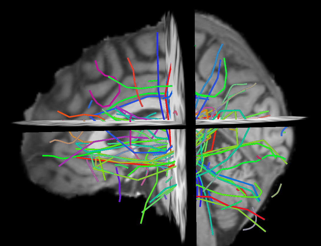
Figure 1: A set of $100$ streamlines, i.e. an example of prototypes, from a full tractography

2 Methods

In the following we present a concise formal description of the dissimilarity projection together with a notion of approximation to quantify how accurate this representation is. Additionally we introduce three strategies for prototype selection that will be compared in Section 3.

2.1 The Dissimilarity Projection

Let $\mathcal{X}$ be the space of the objects of interest, e.g. streamlines, and let $X\in\mathcal{X}$. Let $P_{X}$ be a probability distribution over $\mathcal{X}$. Let $d:\mathcal{X}\times\mathcal{X}\mapsto\mathbb{R}^{+}$ be a distance function between objects in $\mathcal{X}$. Note that $d$ is not assumed to be necessarily metric. Let $\Pi=\{\tilde{X}_{1},\ldots,\tilde{X}_{p}\}$, where $\forall i$ $\tilde{X}_{i}\in\mathcal{X}$ and $p$ is finite. We call each $\tilde{X}_{i}$ as prototype or landmark. The dissimilarity representation/projection is defined as $\phi_{\Pi}^{d}(X):\mathcal{X}\mapsto\mathbb{R}^{p}$ s.t.

$$\phi_{\Pi}^{d}(X)=[d(X,\tilde{X}_{1}),\ldots,d(X,\tilde{X}_{p})]$$ (1)

and maps an object $X$ from its original space $\mathcal{X}$ to a vector of $\mathbb{R}^{p}$.

Note that this representation is a lossy one in the sense that in general it is not possible to exactly reconstruct $X$ from $\phi_{\Pi}^{d}(X)$ because some information is lost during the projection.

We define the distance between projected objects as the Euclidean distance between them: $\Delta_{\Pi}^{d}(X,X^{\prime})=||\phi_{\Pi}^{d}(X)-\phi_{\Pi}^{d}(X^{\prime})||_{2}$, i.e. $\Delta_{\Pi}^{d}:\mathcal{X}\times\mathcal{X}\mapsto\mathbb{R}^{+}$. It is intuitive that $\Delta_{\Pi}^{d}$ and $d$ should be strongly related. In the following sections we will present more details and explanations about this relation.

2.2 A Measure of Approximation

We investigate the relationship between the distribution of distances among objects in $\mathcal{X}$ through $d$ and the corresponding distances in the dissimilarity representation space through $\Delta_{\Pi}^{d}$. We claim that a good dissimilarity representation must be able to accurately preserve the partial order of the distances, i.e. if $d(X,X^{\prime})\leq d(X,X^{\prime\prime})$ then $\Delta_{\Pi}^{d}(X,X^{\prime})\leq\Delta_{\Pi}^{d}(X,X^{\prime\prime})$ for each $X,X^{\prime},X^{\prime\prime}\in\mathcal{X}$ almost always. As a measure of the degree of approximation of the dissimilarity representation we define the Pearson correlation coefficient $\rho$ between the two distances over all possible pairs of objects in $\mathcal{X}$:

$$\boldsymbol{\rho}=\frac{\mathrm{Cov}(d(X,X^{\prime}),\Delta_{\Pi}^{d}(X,X^{\prime}))}{\sigma_{d(X,X^{\prime})}\sigma_{\Delta_{\Pi}^{d}(X,X^{\prime})}}$$ (2)

where $X,X^{\prime}\sim P_{X}$. In practical cases $P_{X}$ is unknown and only a finite sample $S$ is available. We can approximate $\boldsymbol{\rho}$ as the sample correlation $\boldsymbol{r}$ where $X,X^{\prime}\in S$. An accurate approximation of the relative distances between objects in $\mathcal{X}$ results in values of $\boldsymbol{\rho}$ far from zero and close to $1$.

In the literature of the Euclidean embeddings of metric spaces, the term of distortion is used for representing the relation between the distances in the original space and the corresponding ones in the projected space. The embedding is said to have distortion$\leq c$ if for every $x,x^{\prime}\in\mathcal{X}$:

$$d(x,x^{\prime})\geq\Delta_{\Pi}^{d}(x,x^{\prime})\geq\frac{1}{c}d(x,x^{\prime}).$$ (3)

An interesting embedding of metric spaces is described in [7]. It is based on ideas similar to the dissimilarity representation and has the advantage of providing a theoretical bound on the distortion. Unfortunately this embedding is computationally too expensive to be used in practice.

We claim that correlation and distortion target slightly different aspects of the embedding quality, the first focussing on the averaged differences between the original and projected space and the second on the worst case scenario. For this reason we claim that, in the context of machine learning and pattern recognition applications, correlation is a more appropriate measure.

2.3 Strategies for Prototype Selection

The definition of the set of prototypes with the goal of minimising the loss of the dissimilarity projection is an open issue in the dissimilarity space representation literature. In the context of classification problems the policy of random selection of the prototypes was proved to be useful under certain assumptions [1]. In the following we address the issue of choosing the prototypes in order to achieve the desired degree of approximation but we do not restrict to the classification case only. We define and discuss the following policies for prototype selection: random selection, farthest first traversal (FFT) and subset farthest first (SFF). All these policies are parametric with respect to $p$, i.e. the number of prototypes.

2.3.1 Random Selection

In practical cases we have a sample of objects $S=\{X_{1},\ldots,X_{N}\}\subset\mathcal{X}$. This selection policy draws uniformly at random from $S$, i.e. $\Pi\subseteq S$ and $|\Pi|=p$. Note that sampling is without replacement because identical prototypes provide redundant, i.e. useless, information. This policy was first proposed in [4] for seeding clustering algorithms. This policy has the lowest computational complexity $O(1)$.

2.3.2 Farthest First Traversal (FFT)

This policy selects an initial prototype at random from $S$ and then each new one is defined as the farthest element of $S$ from all previously chosen prototypes. The FFT policy is related to the $k$-center problem [6]: given a set $S$ and an integer $k$, what is the smallest $\epsilon$ for which you can find an $\epsilon$-cover of $S$ of size $k$? . The $k$-center problem is known to be an NP-hard [6], i.e. no efficient algorithm can be devised that always returns the optimal answer. Nevertheless FFT is known to be close to the optimal solution, in the following sense: If $T$ is the solution returned by FFT and $T^{*}$ is the optimal solution, then $\max_{x\in S}d(x,T)\leq 2\max_{x\in S}d(x,T^{*})$. Moreover, in metric spaces, any algorithm having a better ratio must be NP-hard [6]. FFT has $O(p|S|)$ complexity. Unfortunately when $|S|$ becomes very large this prototype selection policy becomes impractical.

2.3.3 Subset Farthest First (SFF)

In the context of radial basis function networks initialisation, a scalable approximation of the FFT algorithm, called subset farthest first (SFF), was proposed in [12]. This approximation is also claimed to reduce the chances to select outliers that can lead to a poor representation of large datasets. The SFF policy samples $m=\lceil cp\log p\rceil$ points from $S$ uniformly at random and then applies FFT on this sample in order to select the $p$ prototypes. In [12] it was proved that under the hypothesis of $p$ clusters in $S$, the probability of not having a representative of some clusters in the sample is at most $pe^{-m/p}$. The computational complexity of SFF is $O(p^{2}\log p)$. Note that for large datasets and small $p$ this prototype selection policy has a much lower computational cost than FFT.

3 Experiments

In the following we describe the assessment of the degree of approximation of the dissimilarity representation across different prototype selection policies and different numbers of prototypes. The aim is to investigate the trade-off between accuracy and computational cost. The experiments are carried out on 2D simulated data and on real tractographies reconstructed from dMRI recordings of the human brain.

3.1 Simulated Data

Let $\mathcal{X}=\mathbb{R}^{2}$, $P_{X}=\mathcal{N}(\boldsymbol{\mu},\Sigma)$, $\boldsymbol{\mu}=[0,0]$, $\Sigma=I$, $d(X,X^{\prime})=||X-X^{\prime}||_{2}$, $p=3$ and $\tilde{X}_{1},\tilde{X}_{2},\tilde{X}_{3}\sim P_{X}$. Then $\phi_{\Pi}^{d}(X)=\left[||X-\tilde{X}_{1}||_{2},||X-\tilde{X}_{2}||_{2},||X-\tilde{X}_{3}||_{2}\right]\in\mathbb{R}^{3}$. Figure 2 shows a sample of $50$ points drawn from $P_{X}$ together with the $3$ prototypes $\tilde{X}_{1},\tilde{X}_{2},\tilde{X}_{3}$. Figure 3 shows the sample projected into the dissimilarity space together with the prototypes.

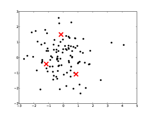
Figure 2: A 2-dimensional example of $50$ points (black circles) drawn from $\mathcal{N}(\boldsymbol{0},I)$ and $3$ prototypes (red stars) drawn from the same pdf.

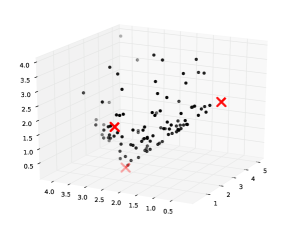
Figure 3: The dissimilarity projection of the dataset and prototypes of Figure 2.

The selection of the prototypes according to different policies is explained in Section 2.3. For SFF we chose $c=3$ in order to have high probability ($>0.95$) of accurately representing $S$ through the subset. Each dataset was projected in the dissimilarity space. The correlation $\boldsymbol{\rho}$ between distances in the original space and the corresponding distances in the projected space was estimated by computing $50$ repetitions of the simulated dataset. The average correlation and one standard deviation for each prototype selection strategy are shown in Figure 4.

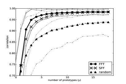
Figure 4: Average correlation between $d$ and $\Delta_{\Pi}^{d}$ across different prototype selection policies and different numbers of prototypes.

In this simulated dataset both SFF and FFT performed significantly better than the random selection, on average. FFT showed a small advantage over SFF when $p<10$.

3.2 Tractography data

We estimated the dissimilarity representation over tractography data from dMRI recordings of the MRI facility at the MRC Cognition and Brain Sciences Unit, Cambridge UK. The dataset consisted of $12$ healthy subjects; $101$ ($+1$, i.e. $b=0$) gradients; $b$-values from 0 to 4000; voxel size: $2.5\times 2.5\times 2.5mm^{3}$. In order to get the tractography we computed the single tensor reconstruction (DTI) and created the streamlines using EuDX, a deterministic tracking algorithm [5] from the DiPy library . We obtained two tractographies using $10^{4}$ and $3\times 10^{6}$ random seed respectively. The first tractography consisted of approximately $10^{3}$ streamlines and the second one of $3\times 10^{5}$ streamlines. An example of a set of prototypes from the largest tractography is shown in Figure 1.

As the distance between streamlines we chose one of the most common, i.e. the symmetric minimum average distance from [14] defined as $d(X_{a},X_{b})=\frac{1}{2}(\delta(X_{a},X_{b})+\delta(X_{b},X_{a}))$ where

$$\delta(X_{a},X_{b})=\frac{1}{|X_{a}|}\sum_{\mathbf{x}_{i}\in X_{a}}\min_{\mathbf{y}\in X_{b}}||\mathbf{x}_{i}-\mathbf{y}||_{2}.$$ (4)

As it is shown in Figure 5 for the case of a tractography of $10^{3}$ streamlines both FFT and SFF ($c=3$) had significantly higher correlation than the random sampling for all numbers of prototypes considered. We confirmed that the SFF selection policy is an accurate approximation of the FFT policy for tractographies. Moreover we noted that after $15-20$ prototypes the correlation reaches approximately $0.95$ on average ($50$ repetitions) and then slightly decreases indicating that a little number of prototypes is sufficient to reach a very accurate dissimilarity representation.

Figure 6 shows the correlation for SFF and the random policy when the tractography has $3\times 10^{5}$ streamlines, i.e. the standard size of a tractography from current dMRI recording techniques. In this case FFT is impractical to be computed because it requires approximately $15$ minutes on a standard desktop computer for a single repetition when $p=50$. The cost of computing SFF is instead the same of the case of $10^{3}$ streamlines, as its computational cost depends only on the number of prototypes. It took $\approx 2$ seconds on standard desktop computer when $p=50$ to compute one repetition. We observed that for $3\times 10^{5}$ streamlines SFF significantly outperformed the random policy and reached the highest correlation of $0.96$ on average ($50$ repetitions) for $15-25$ prototypes.

Note that the figures presented in this section refers to data from subject $1$ of the dMRI dataset. We conducted the same experiments on other subjects obtaining equivalent results. The code to reproduce all the experiments is available at https://github.com/emanuele/prni2012_dissimilarity under an open source license.

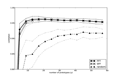
Figure 5: The correlation between of $d$ and $\Delta_{\Pi}^{d}$ over a $10^{3}$ streamlines tractography for different prototype selection policies.

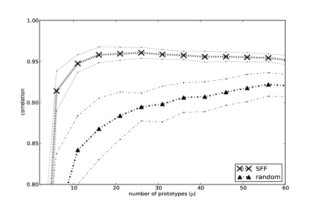
Figure 6: The correlation between of $d$ and $\Delta_{\Pi}^{d}$ for a full tractography of $3\times 10^{5}$ streamlines for the random and SFF prototype selection policies.

4 Discussion

In this document we investigated the degree of approximation of the dissimilarity representation for the goal of preserving the relative distances between streamlines within tractographies. Empirical assessment has been conducted on two different datasets and through various prototype selection methods. All of the results from both simulated data and real tractography data reached correlation $\geq 0.95$ with respect to the distances in the original space. This fact proved that the dissimilarity representation works well for preserving the relative distances. Moreover on tractography data the maximum correlation was reached with just approximately $20-25$ prototypes proving that the dissimilarity representation can produce compact feature spaces for this kind of data.

When comparing the different prototype selection policies we found that FFT had a small advantage over SFF but only when the number of prototypes was very low ($p<10$). Both FFT and SFF always outperformed the random policy. Moreover, since the computational cost of SFF does not increase with the size of the dataset but only with the number of prototypes, we observed that the SFF policy can be easily computed on a standard computer even in the case of a tractography of $3\times 10^{5}$ streamlines. This is different from FFT which is several orders of magnitude slower than SFF, thus computationally less practical.

We advocate the use of the dissimilarity approximation for the Euclidean embedding of tractography data in machine learning and pattern recognition applications. Moreover we strongly suggest the use of the SFF policy to obtain an efficient and effective selection of the prototypes.

References

- [1] Maria-Florina Balcan, Avrim Blum, and Nathan Srebro. A theory of learning with similarity functions. Machine Learning, 72(1):89–112, August 2008.
- [2] P. J. Basser, J. Mattiello, and D. LeBihan. MR diffusion tensor spectroscopy and imaging. Biophysical journal, 66(1):259–267, January 1994.
- [3] Yihua Chen, Eric K. Garcia, Maya R. Gupta, Ali Rahimi, and Luca Cazzanti. Similarity-based Classification: Concepts and Algorithms. Journal of Machine Learning Research, 10:747–776, March 2009.
- [4] E. W. Forgy. Cluster analysis of multivariate data: efficiency vs interpretability of classifications. Biometrics, 21:768–769, 1965.
- [5] E. Garyfallidis. Towards an accurate brain tractography. PhD thesis, University of Cambridge, 2012.
- [6] Dorit S. Hochbaum and David B. Shmoys. A Best Possible Heuristic for the k-Center Problem. Mathematics of Operations Research, 10(2):180–184, May 1985.
- [7] Nathan Linial, Eran London, and Yuri Rabinovich. The geometry of graphs and some of its algorithmic applications. Combinatorica, 15(2):215–245, June 1995.
- [8] Susumu Mori and Peter C. M. van Zijl. Fiber tracking: principles and strategies – a technical review. NMR Biomed., 15(7-8):468–480, 2002.
- [9] Emanuele Olivetti and Paolo Avesani. Supervised segmentation of fiber tracts. In Proceedings of the First international conference on Similarity-based pattern recognition, SIMBAD’11, pages 261–274, Berlin, Heidelberg, 2011. Springer-Verlag.
- [10] E. Pekalska, R. Duin, and P. Paclik. Prototype selection for dissimilarity-based classifiers. Pattern Recognition, 39(2):189–208, February 2006.
- [11] Elzbieta Pekalska, Pavel Paclik, and Robert P. W. Duin. A generalized kernel approach to dissimilarity-based classification. J. Mach. Learn. Res., 2:175–211, 2002.
- [12] D. Turnbull and C. Elkan. Fast recognition of musical genres using RBF networks. Knowledge and Data Engineering, IEEE Transactions on, 17(4):580–584, April 2005.
- [13] Xiaogang Wang, Grimson, and Carl-Fredrik Westin. Tractography segmentation using a hierarchical Dirichlet processes mixture model. NeuroImage, 54(1):290–302, January 2011.
- [14] Song Zhang, S. Correia, and D. H. Laidlaw. Identifying White-Matter Fiber Bundles in DTI Data Using an Automated Proximity-Based Fiber-Clustering Method. Visualization and Computer Graphics, IEEE Transactions on, 14(5):1044–1053, 2008.