The method of constructing models of peer to peer protocols

Abstract

The models of peer to peer protocols are presented with the help of one-step processes. On the basis of this presentation and the method of randomization of one-step processes described method for constructing models of peer to peer protocols. As specific implementations of proposed method the models of FastTrack and Bittorrent protocols are studied.

I Introduction

While constructing stochastic mathematical model there is a certain problem how to introduce the stochastic term which deals not with external impact on the system, but has a direct relationship with the system’s structure. In to order to construct a required mathematical model we will consider the processes occurring in the system as one-step Markov processes.

This approach allows to obtain stochastic differential equations with compatible stochastic and deterministic parts, since they are derived from the same equation. The stochastic differential equations theory allows qualitatively to analyse the solutions of these equations The Runge–Kutta methods are used to obtain the solutions of stochastic differential equations and for illustration of presented results.

In previous studies, the authors developed a method of construction of mathematical model based on one-step stochastic processes, which describe a wide class of phenomena  Demidova et al. (2013); Demidova and Kulyabov (2012). This method presented good results for population dynamic models Demidova et al. (2010, 2012); Demidova (2013). This method is also applicable to some technical problems such as p2p-networks simulation, in particular to the FastTrack and BitTorrent Korolkova and Kulyabov (2013).

The paper proposes to use one-step stochastic processes method in order to construct FastTrack and BitTorrent protocol models and to study stochastic influence on the deterministic model.

II Notations and conventions

1. In this paper the notation of abstract indices is used Penrose and Rindler (1984). Under the given notation, the tensor is denoted by an index (eg, $x^{i}$), and the tensor’s components are denoted by an underlined index (eg, $x^{\underline{\vphantom{j}{i}}}$).

2. Latin indices of the middle of the alphabet (eg, $i$, $j$, $k$) denote system space vectors. Latin indices from the beginning of the alphabet (eg, $a$) are related to the space of Wiener’s process. Latin indices from the end of the alphabet (eg, $p$, $q$) are the indices of the Runge–Kutta methods. Greek indices (eg, $\alpha$) denote a quantity of different interactions in the kinetic equations.

3. A dot over the symbol (eg, $\dot{x}$) denotes time differentiation.

4. A comma in the index denotes the partial derivative with respect to corresponding coordinate.

III One-step processes modeling

Under the one-step process we understand the continuous time Markov processes with integer state space. The transition matrix which allows only transitions between neighboring states. Also, these processes are known as birth-and-death processes.

The state of the system is described by a state vector $x^{i}\in\mathbb{R}^{n}$, where $n$ — system dimension.

The idea of the method is as follows. For the studied system the interaction scheme as a symbolic record of all possible interactions between system elements is introduced. The scheme shows the number and type of elements in certain interaction and the result of the interaction. For this purpose the system state operators are used. The operator $n^{i\alpha}_{j}\in\mathbb{Z}^{n}_{{}\geqslant 0}\times\mathbb{Z}^{n}_{{}\geqslant 0}\times\mathbb{Z}^{s}_{0}$ sets the state of the system before the interaction, and the operator $m^{i\alpha}_{j}\in\mathbb{Z}^{n}_{{}\geqslant 0}\times\mathbb{Z}^{n}_{{}\geqslant 0}\times\mathbb{Z}^{s}_{0}$ — sets the state after the interaction. It is also assumed that in the system $s$ kinds of different interactions may occur, where $s\in\mathbb{Z}_{+}$. As a result of the interaction , the system switches into the $x^{i}\rightarrow x^{i}+r^{i\underline{\vphantom{j}{\alpha}}}_{j}x^{j}$ or $x^{i}\rightarrow x^{i}-r^{i\underline{\vphantom{j}{\alpha}}}_{j}x^{j}$ states, where $r_{j}^{i\alpha}=m_{j}^{i\alpha}-n_{j}^{i\alpha}$.

Let’s introduce transition probabilities from state $x^{i}$ into $x^{i}+r^{i\underline{\vphantom{j}{\alpha}}}_{j}x^{j}$ states (the $x^{i}-r^{i\underline{\vphantom{j}{\alpha}}}_{j}x^{j}$ state). The transition probabilities of are assumed to be proportional to the number of possible interactions between elements.

Based on the interaction schemas and transition probabilities, we create the master equation, decompose it into a series, leaving only the terms up to the second derivative. The resulting equation is the Fokker–Planck equation, which looks like:

$$\frac{\partial p}{\partial t}=-\partial_{i}\left[A^{i}p\right]+\frac{1}{2}\partial_{i}\partial_{j}\left[B^{ij}p\right],$$ (1)

where

$$\begin{gathered}A^{i}:=A^{i}(x^{k},t)=r^{i\underline{\vphantom{j}{\alpha}}}\left[s^{+}_{\underline{\vphantom{j}{\alpha}}}-s^{-}_{\underline{\vphantom{j}{\alpha}}}\right],\\ B^{ij}:=B^{ij}(x^{k},t)=r^{i\underline{\vphantom{j}{\alpha}}}r^{j\underline{\vphantom{j}{\alpha}}}\left[s^{+}_{\underline{\vphantom{j}{\alpha}}}-s^{-}_{\underline{\vphantom{j}{\alpha}}}\right].\end{gathered}$$ (2)

Here $p:=p(x^{i},t)$ is a random variable $x^{i}$ density function, $A^{i}$ — a drift vector, $B^{ij}$ — a diffusion vector.

As it is evident from (2), the Fokker–Planck equation coefficients can be obtained immediately from interaction scheme and transition probabilities, i.e., for practical calculations the master equation is not in need.

To get the more convenient form of the model the corresponding Langevin’s equation is given:

$$\mathrm{d}x^{i}=a^{i}\mathrm{d}t+b^{i}_{a}\mathrm{d}W^{a},$$ (3)

where $a^{i}:=a^{i}(x^{k},t)$, $b^{i}_{a}:=b^{i}_{a}(x^{k},t)$, $x^{i}\in\mathbb{R}^{n}$, $W^{a}\in\mathbb{R}^{m}$ — $m$-dimensional Wiener’s process. It is implemented as $\mathrm{d}W=\varepsilon\sqrt{\mathrm{d}t}$, where $\varepsilon\sim N(0,1)$ — normal distribution with mean equal to$0$ and variance equal to $1$.

The relationship between the equations (1) and (3) is expressed by the following:

$$A^{i}=a^{i},\qquad B^{ij}=b^{i}_{a}b^{ja}.$$ (4)

Thus, for our system description the stochastic differential equation may be derived to from the general considerations. This equation consists of two parts, one of which describes a deterministic behaviour of the system, and other the stochastic one. Furthermore, both sides of the equations are consistent, since they are derived from the same equation (Figure 1).

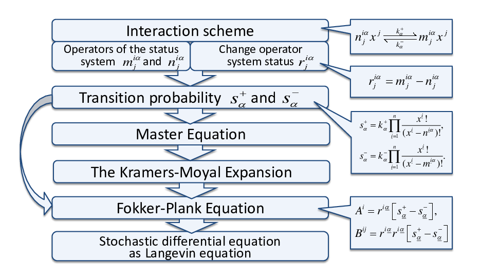
Figure 1: Method’s diagram

IV Fast Track Protocol

Fast Track Protocol is the p2p network protocol for Internet file sharing. The file can be downloaded only from peers which possess the whole file. FastTrack was originally implemented in the KaZaA software. It has a decentralized topology that makes it very reliable. All FastTrack users are divided into two classes: supernodes and ordinary nodes. The supernodes allocation is one of the functions of FT protocol. Supernodes are those with fast network connection, high-bandwidth and possibility of a fast data processing. The users themselves do not know that their computer has been designated as a supernode.

To upload a file, a node sends a request to the supernode, which, in its turn, communicates with the other nodes, etc. So, the request extends to a certain level protocol network which is called a lifetime request. After as the desired file is found, it is directly sent to the node bypassing the supernode from the node possessing the necessary file Liang et al. (2006); Ding et al. (2006).

IV.1 FastTrack modeling

Assume that the file consists of one part Thus, during one interaction, the node desiring to download it can download the entire file at once. When the download is completed, the node becomes supernode.

Let $N$ denote the new node, $L$ — supernode and $\beta$ — interaction coefficient. The new nodes appear with the intensity of $\lambda$, and the supernodes leave the system with the intensity of $\mu$. Then the scheme of interaction and vector $\mathbf{r}$ are:

$$\begin{cases}0\xrightarrow{\lambda}N,&r^{\underline{\vphantom{j}{i}}1}=(1,0)\\ N+L\xrightarrow{\beta}2L,&r^{\underline{\vphantom{j}{i}}2}=(-1,1)\\ L\xrightarrow{\mu}0,&r^{\underline{\vphantom{j}{i}}3}=(0,-1).\end{cases}$$ (5)

The first line in the diagram describes the a new client appearance in the system. The second line reflects the interaction of a new client and a seed. After this interaction a new seed appears. And the third line indicates the departure of the seed from the system. Let us introduce the transition probabilities:

$$\begin{gathered}s^{+}_{1}(n,l)=\lambda\\ s^{+}_{2}(n,l)=\beta nl\\ s^{+}_{3}(n,l)=\mu l.\end{gathered}$$ (6)

It is possible now to write out the Fokker-Planck equation for our model:

$$\frac{\partial p(n,l)}{\partial t}={\partial_{i}}(A^{i}(n,l)p(n,l))+\frac{1}{2}{\partial_{i}\partial_{j}}(B^{ij}(n,l)p(n,l)),$$ (7)

where the drift vector and diffusion matrix are follows:

$$\begin{gathered}A^{i}:=A^{i}(x^{k},t)=r^{i\underline{\vphantom{j}{\alpha}}}s^{+}_{\underline{\vphantom{j}{\alpha}}}(n,l),\\ B^{i}:=B^{ij}(x^{k},t)=r^{i\underline{\vphantom{j}{\alpha}}}r^{i\underline{\vphantom{j}{\alpha}}}s^{+}_{\underline{\vphantom{j}{\alpha}}}(n,l),\underline{\vphantom{j}{\alpha}}=1,2,3.\end{gathered}$$ (8)

At last we get:

$$\begin{gathered}\mathbf{A}=\begin{pmatrix}1\\ 0\end{pmatrix}\lambda+\begin{pmatrix}-1\\ 1\end{pmatrix}\beta nl+\begin{pmatrix}0\\ -1\end{pmatrix}\mu l=\begin{pmatrix}\lambda-\beta nl\\ \beta nl-\mu l\end{pmatrix},\\ \begin{multlined}\mathbf{B}=\begin{pmatrix}1\\ 0\end{pmatrix}(1,0)\lambda+\begin{pmatrix}-1\\ 1\end{pmatrix}(-1,1)\beta nl+\begin{pmatrix}0\\ -1\end{pmatrix}(0,-1)\mu l=\\ =\begin{pmatrix}\lambda+\beta nl&-\beta nl\\ -\beta nl&\beta nl+\mu l\end{pmatrix}.\end{multlined}\mathbf{B}=\begin{pmatrix}1\\ 0\end{pmatrix}(1,0)\lambda+\begin{pmatrix}-1\\ 1\end{pmatrix}(-1,1)\beta nl+\begin{pmatrix}0\\ -1\end{pmatrix}(0,-1)\mu l=\\ =\begin{pmatrix}\lambda+\beta nl&-\beta nl\\ -\beta nl&\beta nl+\mu l\end{pmatrix}.\end{gathered}$$ (9)

The stochastic differential equation in its Langevin’s form can be derived by using an appropriate formula.

IV.2 Deterministic behavior

Since the drifts vector $A$ completely describes the deterministic behavior of the system, it is possible to derive an ordinary differential equations system, which describes the population dynamics of new clients and seeds.

$$\left\{\begin{aligned} \frac{dn}{dt}&=\lambda-\beta nl\\ \frac{dl}{dt}&=\beta nl-\mu l\end{aligned}\right.$$ (10)

IV.2.1 Steady-states

Let us find steady-states of the system (10) from the following system of equations:

$$\left\{\begin{aligned} \lambda-\beta nl&=0\\ \beta nl-\mu l&=0\end{aligned}\right.$$ (11)

The system (10) has the only one steady state:

$$(\bar{n},\bar{l})=\left(\frac{\mu}{\beta},\frac{\lambda}{\mu}\right)$$ (12)

.

To linearize the system (10), let $n=\bar{n}+\xi$, $l=\bar{l}+l\eta$, where $\bar{n}$ and $\bar{l}$ are coordinates of stability points, $\xi$ and $\eta$ are small parameters

$$\left\{\begin{aligned} \frac{d\xi}{dt}&=-\beta\bar{n}\eta-\beta\bar{l}\xi\\ \frac{d\eta}{dt}&=\beta\bar{n}\eta+\beta\bar{l}\xi-\mu\eta\end{aligned}\right.$$ (13)

In the neighborhood of the equilibrium point, the linearized system is presented as following::

$$\left\{\begin{aligned} \frac{d\xi}{dt}&=-\mu\eta\frac{\beta\lambda}{\mu}\xi\\ \frac{d\eta}{dt}&=\frac{\beta\lambda}{\mu}\xi\end{aligned}\right.$$ (14)

Now we may find the eigenvalues of the characteristic equation:

$$s^{2}+\frac{\beta\lambda}{\mu}s+\beta\lambda=0.$$ (15)

The roots of this characteristic equation:

$$s_{1,2}=\frac{1}{2}\left(-\frac{\beta\lambda}{\mu}\pm\sqrt{\left(\frac{\beta\lambda}{\mu}\right)^{2}-4\beta\lambda}\right).$$ (16)

Thus, depending on the choice of parameters, the critical point has different types. In the case when $\beta\lambda<4\mu^{2}$, the critical point represents a stable focus, while in the reverse case — a steady node. In both the cases, the singular point is a stable one because the real part of the roots of the equation is negative. Thus, depending on the choice of coefficient, the change of values of the variables can occur in one of two trajectories.

In the case when the critical point represents a focus, the damped oscillations of the nodes and supernodes quantity occur  2. And if the critical point is node, there are no oscillations in the trajectories 3. Phase portraits of the system for each of the two cases are plotted, respectively, in Figs.  4 and  5.

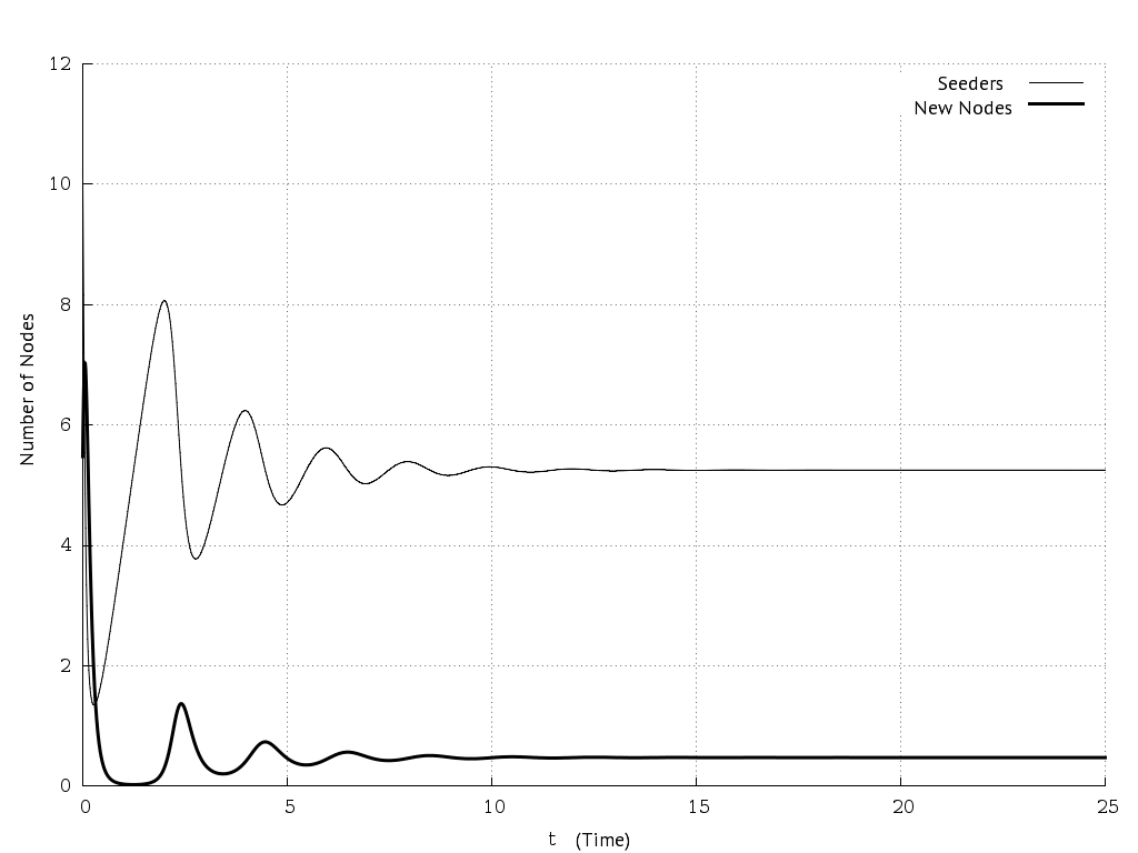
Figure 2: The time dependence of the nodes and seeds quantity in the Fast Track network for the deterministic case $\beta\lambda<4\mu^{2}$.

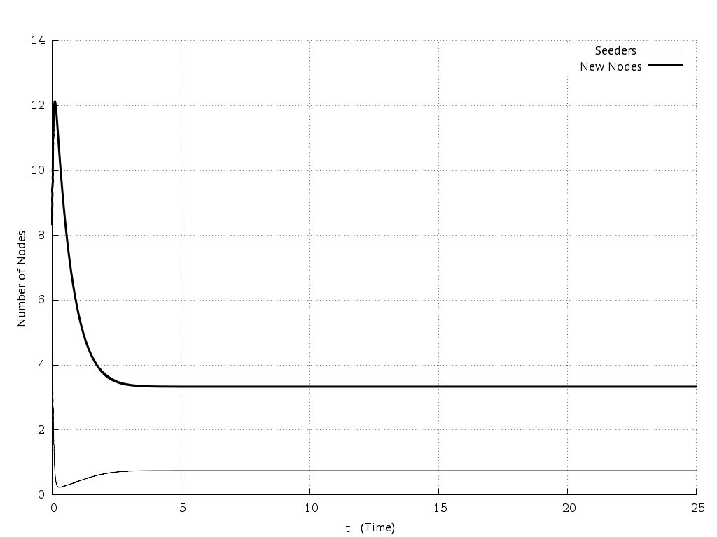
Figure 3: The time dependence of the nodes and seeds quantity in Fast Track network for the deterministic case $\beta\lambda>4\mu^{2}$.

Figure 4: Phase portraits of a deterministic Fast Track system with various deviations $(\Delta x,\Delta y)$ from stationary point if $\beta\lambda<4\mu^{2}$.

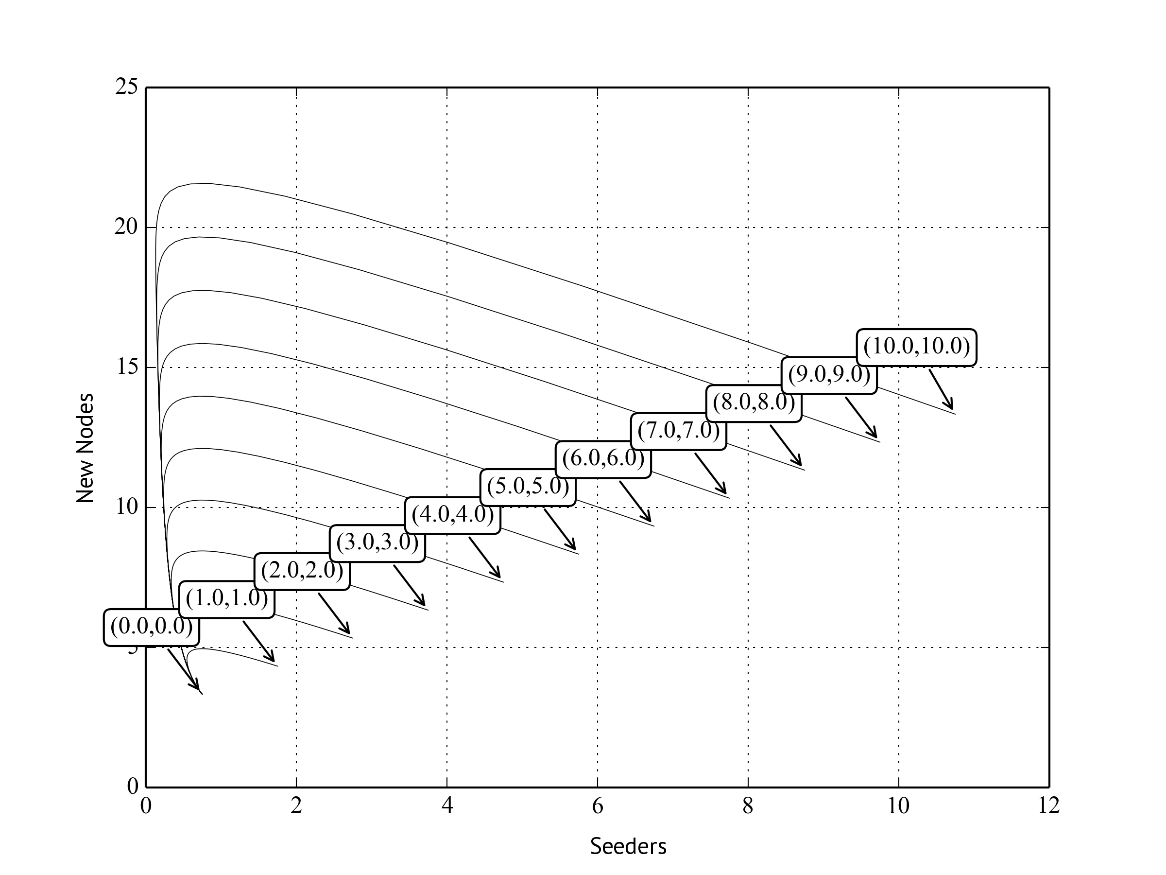
Figure 5: Phase portraits of a deterministic Fast Track system with various deviations $(\Delta x,\Delta y)$ from stationary point if $\beta\lambda>4\mu^{2}$.

IV.2.2 Numerical simulation of the stochastic model

To illustrate the obtained results the numerical modelling of stochastic differential equation in the Langevin’s form was performed. The extension of Runge-Kutta methods for stochastic differential equations was applied Tocino and Ardanuy (2002); Debrabant and Röbler (2008), and a Fortran program for this extension was written. The results are presented on Figures 7 and 8.

Figures 7 and 8 clearly indicate that small stochastic terms do not substantially affect the behaviour of the system in the stationary point neighbourhood. The stochastic term influence exists only on the early evolution of the system. After a relatively short period of time, the system enters the steady-state regime and differs little from the deterministic case.

Conclusions

The obtained results indicate that the stochastic introduction in the steady-state regime has little effect on the behaviour of the system. So, the deterministic model provides the appropriate results.

Furthermore, the proposed method allows to extend the framework of the tools used for the analysis, so is becomes possible to use ordinary stochastic differential equation (Langevin) and partial differential equation (Fokker-Planck) simultaneously. Furthermore, as the above example indicates, in some cases a deterministic approach defined by the diffusion matrix is sufficient.

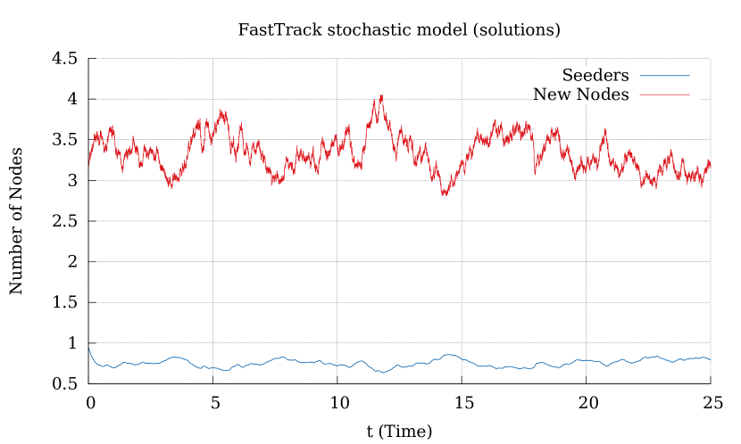
Figure 6: The time dependence of new nodes and seeds quantity in the FastTrack network for the stochastic case.

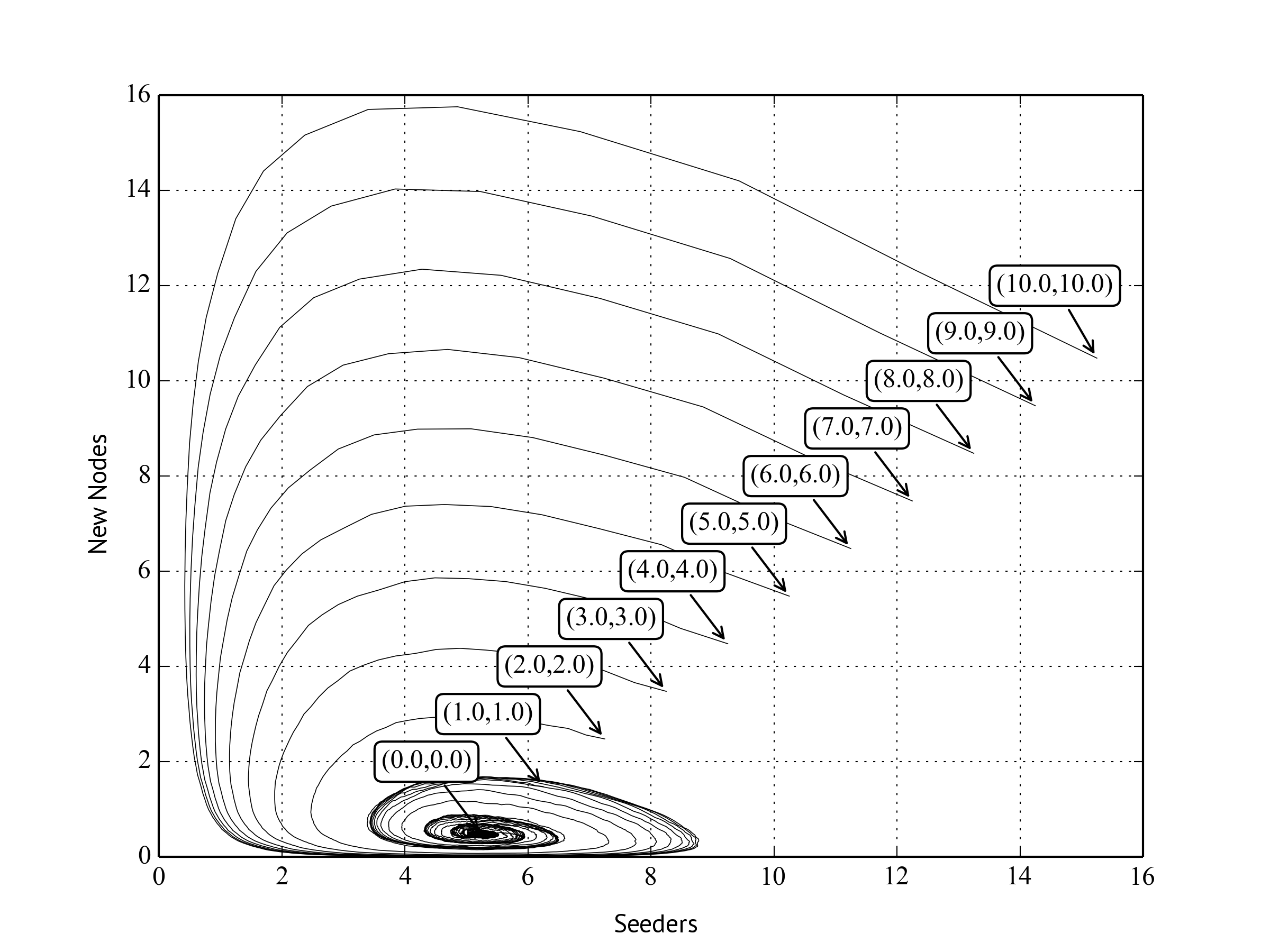
Figure 7: Phase trajectories of the stochastic FastTrack model with various deviations $(\Delta x,\Delta y)$ from the stationary point $\beta\lambda>4\mu^{2}$.

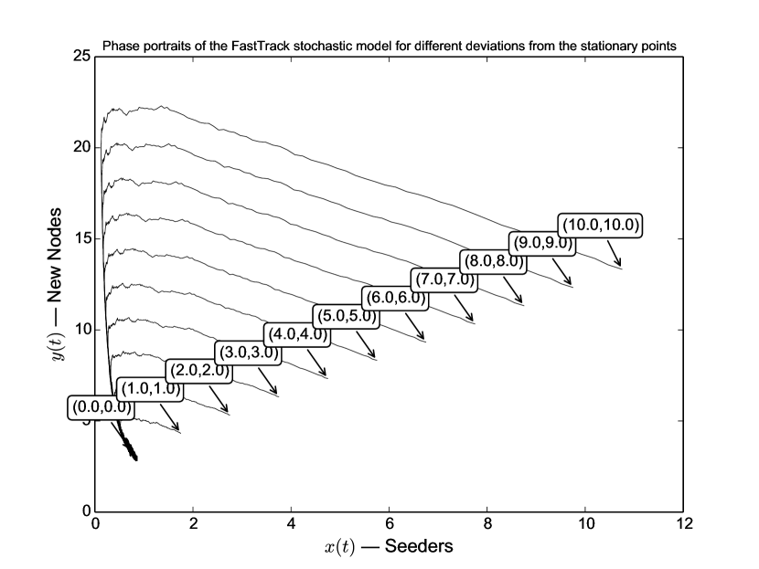
Figure 8: Phase trajectories of the stochastic FastTrack model with various deviations $(\Delta x,\Delta y)$ from the stationary point $\beta\lambda>4\mu^{2}$.

V BitTorrent protocol

BitTorrent is the p2p-network protocol for file sharing over the Internet. Files are transferred by chunks. Each torrent-client simultaneously downloads the needed chunks from one node and uploads available chunks to another node. It makes the BitTorrent protocol more flexible then the FastTrack one.

V.1 Modeling

First, we consider a simplified model of a closed system, where the numbers of leechers and seeders are constant. Furthermore, we assume that the file consists of one chunk. Thus, the leecher downloads the file during only one time step and then becomes a seeder.

Let $N$ denote a new leecher, $C$ —seeder, and $\beta$ — interaction coefficient. Then the interaction scheme will be:

$$N+C\xrightarrow{\beta}2C,\qquad r^{\underline{\vphantom{j}{i}}2}=(-1,1).$$ (17)

The scheme reflects that after the leecher interaction with the seeder, the leecher disappears and another seeder appears.

Next, let $n$ be the number of new nodes, and $c$ — the number of seeders in the system.

The transition probabilities:

$$s^{+}(n,c)=\beta nc.$$ (18)

The Fokker–Planck’s equation for this model:

$$\frac{\partial p(n,c)}{\partial t}={\partial_{i}}(A^{i}(n,c)p(n,c))+\frac{1}{2}{\partial_{i}\partial_{j}}(B^{ij}(n,c)p(n,c)),$$ (19)

where the drift vector and the diffusion matrix are presented as following:

$$\begin{gathered}A^{i}(n,c)=r^{i\underline{\vphantom{j}{\alpha}}}s^{+}_{\underline{\vphantom{j}{\alpha}}}(n,l),\\ B^{i}(n,c)=r^{i\underline{\vphantom{j}{\alpha}}}r^{i\underline{\vphantom{j}{\alpha}}}s^{+}_{\underline{\vphantom{j}{\alpha}}}(n,l).\end{gathered}$$ (20)

Thus, we obtain:

$$\begin{gathered}\mathbf{A}=\begin{pmatrix}-1\\ 1\end{pmatrix}\beta nc+=\begin{pmatrix}-\beta nl\\ \beta nl\end{pmatrix},\\ \begin{multlined}\mathbf{B}=\begin{pmatrix}-1\\ 1\end{pmatrix}(-1,1)\beta nc=\begin{pmatrix}\beta nc&-\beta nc\\ -\beta nc&\beta nc\end{pmatrix}.\end{multlined}\mathbf{B}=\begin{pmatrix}-1\\ 1\end{pmatrix}(-1,1)\beta nc=\begin{pmatrix}\beta nc&-\beta nc\\ -\beta nc&\beta nc\end{pmatrix}.\end{gathered}$$ (21)

The stochastic differential equation in the Langevin’s form can be obtained with the help of the appropriate formula.

It is also possible to write out differential equations which describe the deterministic behaviour of the system:

$$\left\{\begin{aligned} \frac{dn}{dt}&=-\beta nc\\ \frac{dc}{dt}&=\beta nc\end{aligned}\right.$$ (22)

Next, we consider the open system in which new clients appear with the intensity $\lambda$, and seeders leave it with the intensity $\mu$. Now, the scheme of interaction has the form of:

$$0\xrightarrow{\lambda}N, r^{\underline{\vphantom{j}{i}}1}=(1,0),$$ (23)

$$N+C\xrightarrow{\beta}2C, r^{\underline{\vphantom{j}{i}}2}=(-1,1),$$

$$C\xrightarrow{\mu}0, r^{\underline{\vphantom{j}{i}}3}=(0,-1).$$

The first line in the scheme describes the appearance of the new peer in the system, the second line describes the interactions between the new peer and the seeder, after which a new seeder appears. And the third line meaning is that the seeder leaves the system.

Let $n$ denote the number of new clients and $c$ — the number of seeders in the system.

This system is equivalent to the Fast Track model up to notation.

Now consider a system in which downloaded files consist of $m$ chunks. The system consists of:

• Peers ($N$) are the clients without any chunk of the file.

• Leechers ($L$) are the clients who have already downloaded a number of chunks of the file and can share them with new peers or other leechers.

• Seeders ($C$) are the clients who have the whole file and they only can share the file.

In addition, $n$ is the number of new peers, and $c$ — number of seeders in the system, $l_{i}$ — number of leechers with exactly $i$ chunks of the file, where $i=\overline{i,n-1}$. Also, let $\bar{L}_{i}$ be the number of leechers with any chunk of the file of interest for leecher $L_{i}$ and the $\bar{l}_{i}$ is their amount.

For this scheme it is possible to write out the following types of relations:

$$0\xrightarrow{\lambda} N,$$ (24)

$$N+C\xrightarrow{\beta} L_{1}+C,$$

$$N+L_{i}\xrightarrow{\beta_{i}} L_{1}+L_{i},$$

$$L_{i}+\bar{L}_{i}\xrightarrow{\delta_{i}} L_{i+1}+\bar{L}_{i},$$

$$L_{i}+C\xrightarrow{\gamma_{i}} L_{i+1}+C,$$

$$L_{m-1}+\bar{L}_{m-1}\xrightarrow{\gamma_{m-1}} C+\bar{L}_{m-1},$$

$$L_{m-1}+C\xrightarrow{\gamma} 2C,$$

$$C\xrightarrow{\mu} 0.$$

On every interaction step one chunk of file is transferred from one peer to another. The first relation describes the appearance of a new peer in a system with the intensity $\lambda$.

The second and third relations describe the interaction of a new peer with a seeder or a leecher with the interaction coefficients $\beta$ and $\beta i$, $(i=\overline{i,m-1})$. As the result of interaction, the peer transforms into a leecher from the $L_{1}$ class. The fourth and fifth relations describe the leecher $L_{i}$ interaction with the seeder and other leechers with the coefficients $\delta_{i}$ and $\gamma_{i}$ $(i=\overline{i,m-2})$. As the result of this interaction, the leecher gets one chunk of a file and becomes the $L_{i+1}$-class leacher. The sixth and seventh relations describe the transformation of leecher into seeders with the coefficients $\gamma_{m-1}$ and $\gamma$ (the leecher downloads the last file chunk). The last relation describes the seeder departure from the system with the intensity $\mu$.

The vectors $r^{i\underline{\vphantom{j}{\alpha}}}=(n,l_{1},l_{2},...,l_{m-1},c)$ and transition probabilities $s^{+}_{\underline{\vphantom{j}{\alpha}}}$:

$$\begin{gathered}r^{1}=(1,0,0,...,0),\\ r^{2}=r_{i}^{3}=(-1,1,0,...,0),i=\overline{i,m-1}\\ r_{i}^{4}=r_{i}^{5}=(0,...,-1,1,...,0),i=\overline{i,m-2}\\ r^{6}=r^{7}=(0,0,...,-1,1),\\ r^{8}=(0,0,...,-1).\end{gathered}$$ (25)

$$\begin{gathered}s^{+}_{1}=\lambda,\\ s^{+}_{2}=\beta nc,\\ s^{+}_{3i}=\beta_{i}nl_{i},\\ s^{+}_{4i}=\delta_{i}l_{i}\bar{l}_{i},i=\overline{i,m-1}\\ s^{+}_{5i}=\gamma_{i}l_{i}c,i=\overline{i,m-2}\\ s^{+}_{6}=\gamma_{m-1}l_{m-1}\bar{l}_{m-1},\\ s^{+}_{7}=\gamma l_{m-1}c,\\ s^{+}_{8}=\mu c.\\ \end{gathered}$$ (26)

For this model, which is similar to the previous one, we can write out the Fokker-Planck’s equation. But for deterministic behaviour description, it’s enough to write out the matrix $A$.

$$\mathbf{A}=\begin{pmatrix}\lambda-\beta nc-\sum_{i=1}^{m-1}\beta_{i}nl_{i}\\ \beta nc+\sum_{i=1}^{m-1}\beta_{i}nl_{i}-\delta_{1}l_{1}\bar{l}_{1}-\gamma_{1}l_{1}c\\ \delta_{1}l_{1}\bar{l}_{1}+\gamma_{1}l_{1}c-\delta_{2}l_{2}\bar{l}_{2}-\gamma_{2}l_{2}c\\ \ldots\\ \begin{multlined}\delta_{m-2}l_{m-2}\bar{l}_{m-2}+\gamma_{m-2}l_{m-2}c-{}\\ {}-\delta_{m-1}l_{m-1}\bar{l}_{m-1}-\gamma_{m-1}l_{m-1}c\end{multlined}\delta_{m-2}l_{m-2}\bar{l}_{m-2}+\gamma_{m-2}l_{m-2}c-{}\\ {}-\delta_{m-1}l_{m-1}\bar{l}_{m-1}-\gamma_{m-1}l_{m-1}c\\ \delta_{m-1}l_{m-1}\bar{l}_{m-1}+\gamma_{m-1}l_{m-1}c-\mu c\end{pmatrix}.$$ (27)

As a result, we obtain a system of differential equations describing the dynamics of new peers, leechers and seeders:

$$\left\{\begin{gathered}\frac{dn}{dt}=\lambda-\beta nc-\sum_{i=1}^{m-1}\beta_{i}nl_{i},\\ \frac{dl_{1}}{dt}=\beta nc+\sum_{i=1}^{m-1}\beta_{i}nl_{i}-\delta_{1}l_{1}\bar{l}_{1}-\gamma_{1}l_{1}c,\\ \frac{dl_{2}}{dt}=\delta_{1}l_{1}\bar{l}_{1}+\gamma_{1}l_{1}c-\delta_{2}l_{2}\bar{l}_{2}-\gamma_{2}l_{2}c,\\ \ldots\\ \begin{multlined}\frac{dl_{m-1}}{dt}=\delta_{m-2}l_{m-2}\bar{l}_{m-2}+\gamma_{m-2}l_{m-2}c-{}\\ {}-\delta_{m-1}l_{m-1}\bar{l}_{m-1}-\gamma_{m-1}l_{m-1}c,\end{multlined}\frac{dl_{m-1}}{dt}=\delta_{m-2}l_{m-2}\bar{l}_{m-2}+\gamma_{m-2}l_{m-2}c-{}\\ {}-\delta_{m-1}l_{m-1}\bar{l}_{m-1}-\gamma_{m-1}l_{m-1}c,\\ \frac{dc}{dt}=\delta_{m-1}l_{m-1}\bar{l}_{m-1}+\gamma_{m-1}l_{m-1}c-\mu c.\end{gathered}\right.$$ (28)

Let’s suppose that $\delta=\delta_{1}=\delta_{2}=...=\delta_{m-1}=const$, then let’s sum the equations in our system from the second one to the $m+1$-th. If we denote leechers and seeders as $l=l_{1}+l_{2}+...+l_{m-1}+c$ the system of the equations may be simplified as follows:

$$\left\{\begin{aligned} \frac{dn}{dt}&=\lambda-\beta n(l+c),\\ \frac{d(l+c)}{dt}&=\beta n(l+c)-\mu c.\end{aligned}\right.$$ (29)

VI Conclusion

1. In this paper the method of stochastic models construction by use of one-step stochastic processes is described. The proposed method provides an universal algorithm of deriving stochastic differential equations for such systems. It’s also shown that there are two way of stochastic system’s description: with the help of partial differential equation (Fokker-Plank) and ordinary differential equations (Langevin).

2. In order to study influence of the stochastic term of an equation the Fast Track and Bittorrent protocol models were discussed. The results of this study indicate, that near the stationary points the stochastic influence is minimal, and that’s because the deterministic model gives very good results. In addition, as it was shown by the above example, in some cases, in order to examine the system it is enough to study its deterministic approximation, which is described by the drift matrix.

References

- Liang et al. [2006] J. Liang, R. Kumar, and K. W. Ross. The FastTrack overlay: a measurement study. Computer Networks, (50(6)):842–858, 2006.
- Penrose and Rindler [1984] R. Penrose and W. Rindler. Spinors and Space-Time: Two-Spinor Calculus and Relativistic Fields, volume 1. Cambridge University Press, 1984.
- Debrabant and Röbler [2008] K. Debrabant and A. Röbler. Classification of Stochastic Runge–Kutta Methods for the Weak Approximation of Stochastic Differential Equations. Mathematics and Computers in Simulation, 77(4):408–420, 2008. ISSN 0378-4754. doi: http://dx.doi.org/10.1016/j.matcom.2007.04.016.
- Ding et al. [2006] C. H. Ding, S. Nutanong, and R. Buyya. Peer-to-peer networks for content sharing. Journal of Systems Architecture, (52):737–772, 2006.
- Korolkova and Kulyabov [2013] A. V. Korolkova and D. S. Kulyabov. Methods of Stochastization of Mathematical Models on the Example of Peer to Peer Networks. In A Scientific Session NRNU MEPHI–2013, page 131, Moscow, 2013. MEPHI.
- Demidova et al. [2013] A. V. Demidova, A. V. Korolkova, D. S. Kulyabov, and L. A. Sevastianov. The Method of Stochastization of One-Step Processes. In Mathematical Modeling and Computational Physics, page 67. JINR, 2013.
- Demidova [2013] A. V. Demidova. The method of stochastization of mathematical models for the example of the ‘‘predator-prey’’. In A Scientific Session NRNU MEPHI-2013, page 127, 2013. in Russian.
- Tocino and Ardanuy [2002] A. Tocino and R. Ardanuy. Runge–Kutta Methods for Numerical Solution of Stochastic Differential Equations. Journal of Computational and Applied Mathematics, 138(2):219–241, 2002. ISSN 0377-0427. doi: http://dx.doi.org/10.1016/S0377-0427(01)00380-6. URL http://www.sciencedirect.com/science/article/pii/S0377042701003806.
- Demidova et al. [2012] A. V. Demidova, D. S. Kulyabov, and L. A. Sevastianov. The agreed stochastic term in population models. In XI Belarusian Mathematical Conference, page 39, Minsk, 2012. Institute of Mathematics of the National Academy of Sciences of Belarus. in Russian.
- Demidova et al. [2010] A. V. Demidova, L. A. Sevastianov, and D. S. Kulyabov. Application of Stochastic Differencial Equations to Model Population Systems. In Third International Conference on Mathematical Modelling of Social and Economical Dynamics MMSED-2010, pages 92–94. Russian State Social University, 2010. in Russian.
- Demidova and Kulyabov [2012] A. V. Demidova and D. S. Kulyabov. The Introduction of an Agreed Term in the Equation of Stochastic Population Model. Bulletin of Peoples Friendship University of Russia. Series Mathematics. Information Sciences. Physics, (3):69–78, 2012. In Russian.