Using FUV to IR Variability to Probe the Star–Disk Connection in the Transitional Disk of GM Aur

Laura Ingleby¹¹affiliation: Department of Astronomy, Boston University, 725 Commonwealth Avenue, Boston, MA 02215, USA; lingleby@bu.edu , Catherine Espaillat¹¹affiliation: Department of Astronomy, Boston University, 725 Commonwealth Avenue, Boston, MA 02215, USA; lingleby@bu.edu , Nuria Calvet²²affiliation: Department of Astronomy, University of Michigan, 830 Dennison Building, 500 Church Street, Ann Arbor, MI 48109, USA , Michael Sitko³³affiliation: Department of Physics, University of Cincinnati, Cincinnati OH 45221, USA , Ray Russell⁴⁴affiliation: The Aerospace Corporation, Los Angeles, CA 90009, USA , Elizabeth Champney³³affiliation: Department of Physics, University of Cincinnati, Cincinnati OH 45221, USA

Abstract

We analyze 3 epochs of ultraviolet (UV), optical and near-infrared (NIR) observations of the Taurus transitional disk GM Aur using the Hubble Space Telescope Imaging Spectrograph (STIS) and the Infrared Telescope Facility SpeX spectrograph. Observations were separated by one week and 3 months in order to study variability over multiple timescales. We calculate accretion rates for each epoch of observations using the STIS spectra and find that those separated by one week had similar accretion rates ( $\sim 1\times 10^{-8}$ $M_{\sun}\,yr^{-1}$ ) while the epoch obtained 3 months later had a substantially lower accretion rate ( $\sim 4\times 10^{-9}$ $M_{\sun}\,yr^{-1}$ ). We find that the decline in accretion rate is caused by lower densities of material in the accretion flows, as opposed to a lower surface coverage of the accretion columns. During the low accretion rate epoch we also observe lower fluxes at both far UV (FUV) and IR wavelengths, which trace molecular gas and dust in the disk, respectively. We find that this can be explained by a lower dust and gas mass in the inner disk. We attribute the observed variability to inhomogeneities in the inner disk, near the corotation radius, where gas and dust may co-exist near the footprints of the magnetospheric flows. These FUV–NIR data offer a new perspective on the structure of the inner disk, the stellar magnetosphere, and their interaction.

Accretion, accretion disks, Stars: Circumstellar Matter, Stars: Pre Main Sequence

1 Introduction

The early picture of static, axisymmetric circumstellar disks irradiated by a constant luminosity T Tauri star has evolved to include disk warps, fluctuating accretion of material in the disk and ever changing emission properties of the central star, among other dynamic processes. Each of these manifest themselves in T Tauri light curves as variability. Warps block light from the star, causing optical dips (Bouvier et al., 1999; Alencar et al., 2010; Morales-Calderón et al., 2011; Cody et al., 2014) while variable accretion may be seen as bursts in optical and ultraviolet light curves (Herbst et al., 1994; Stauffer et al., 2014) or changing widths and intensities of emission lines produced by accretion (Costigan et al., 2012; Chou et al., 2013; Dupree et al., 2014). Activity cycles in the star may cause long timescale X-ray variability (Micela & Marino, 2003), while short, strong X-ray bursts are produced by solar-like flares (Wolk et al., 2005). Depending on the cause, variability is seen as periodic or stochastic, lasting for minutes or slowly varying over a period of years. With all these characteristics of T Tauri light curves, often with multiple phenomena occurring simultaneously, explaining variability is complicated, especially if the time sampling is low or the wavelength coverage is limited.

In addition, the radial structure of dust in the disk is not always continuous. Along with full disks, those with gaps or holes in the dust (pre-transitional or transitional, respectively) are known to exist (Strom et al., 1989; Skrutskie et al., 1990; Calvet et al., 2002; Espaillat et al., 2007; Andrews et al., 2011) all thought to eventually end up as debris disks with little gas and processed dust (Zuckerman, 2001; Chen et al., 2006; Matthews et al., 2014). Planet formation, photoevaporation of the disk by the central star or viscous evolution, and settling have all been invoked to explain these structures observed in the dust (Espaillat et al., 2014; Zhu et al., 2011; Owen et al., 2012). Gaps and holes in the disk can alter interpretations of T Tauri variability, as processes relevant to full disks appear differently in transitional disks. For example, a warp in the disk wall at the sublimation temperature may not be a contributor to the light curves of transitional disks, which have walls at much larger radii. Therefore, varied dust distributions add an additional complication to the interpretation of T Tauri variability.

Here, we analyze variability in the transitional disk GM Aur over 3 epochs of observation with full wavelength coverage from the far-ultraviolet (FUV) to near-infrared (NIR), all obtained within one day. While photometric variability studies focusing on one or multiple wavelength regimes are significant in number, there are few, if any, variability studies with such extensive spectral coverage. GM Aur is a K5 source in the Taurus molecular cloud, initially suspected to be a transitional disk (Marsh & Mahoney, 1992; Koerner et al., 1993; Chiang & Goldreich, 1999) and later established as having an inner clearing of optically thick dust, though with a small amount of submicron-sized optically thin dust remaining, using Spitzer Infrared Spectrograph (IRS) observations (Calvet et al., 2005; Espaillat et al., 2010). Sub-millimeter observations confirmed that GM Aur has an inner hole in the dust, with a radius of $\sim$ 20 AU (Hughes et al., 2009; Andrews et al., 2011). Rice et al. (2003) showed that transitional disk IRS spectra may be produced by clearing of disk material by planets over a range of disk radii. While photoevaporation models can also produce inner disk holes, the size of the cavity in GM Aur and the presence of remaining gas and small dust are better understood in a planet formation scenario (Owen et al., 2010). In addition to existing long wavelength observations of GM Aur, far and near ultraviolet (FUV and NUV, respectively) spectra have provided glimpses of the gas in the disk of GM Aur (Ardila et al., 2013) and the emission produced in an accretion shock at the stellar surface (Ingleby et al., 2013).

In §2, we discuss the UV, optical and near- IR observations used in our analysis. In §3 we outline our modeling procedures for each epoch of GM Aur data, including accretion shock modeling, comparison of IR fluxes to models of the emission from dust in the disk, and a discussion of the molecular contribution to the FUV. Finally, in §4 we propose a scenario to explain the variability of these spectra.

2 Observations

2.1 STIS

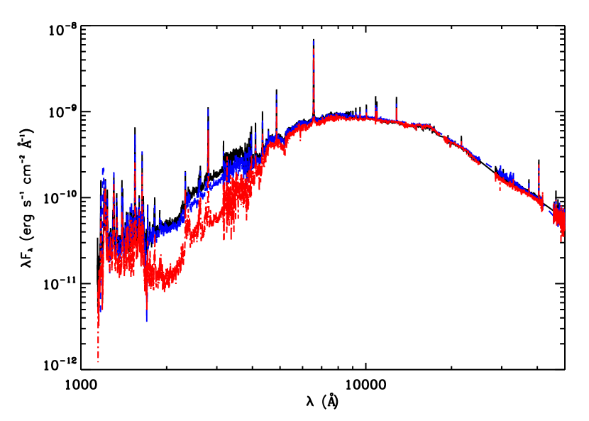
GM Aur was observed during 3 epochs, referred to as GM_1, GM_2 and GM_3 in the following analysis, between September 2011 and January 2012 in GO program 11608 (PI: N. Calvet) with the Space Telescope Imaging Spectrograph (STIS). The observations were separated by 1 week (GM_1 to GM_2) and 3 months (GM_1 to GM_3) in order to study variability on short and long timescales. Spectra were obtained from the FUV to optical, approximately 1100 Å to 1 $\mu$ m, utilizing a combination of STIS gratings. The UV gratings, G140L and G230L used the MAMA detector and provided spectra between 1150 and 3180 Å with resolution, $R$ , ranging between 500 and 1,440. G430L and G750L used the CCD detector and covered 2900 to 10,270 Å with $R\sim 530-1,040$ . We used data products produced through the STScI calstis reduction pipeline for our analysis. A log of all STIS observations is provided in Table 1 and the spectra are plotted in Figure 1, combined with IR data obtained from SpeX, discussed in §2.2.

Refer to caption — Figure 1: UV, optical and IR spectra of GM Aur. Three epochs of observations are shown as solid black (GM_1), dashed blue (GM_2) and dot-dashed red (GM_3) lines. Gaps in the near- IR SpeX data are regions where data is not shown due to poor telluric subtraction.

2.2 SpeX

GM Aur was observed using the SpeX spectrograph (Rayner et al., 2003) on NASA’s Infrared Telescope Facility (IRTF). The SpeX observations were obtained using the cross-dispersed (hereafter XD) echelle gratings in both short-wavelength mode (SXD) covering 0.8-2.4 µm with a resolution of $\sim$ 2000 and long-wavelength mode (LXD) covering 2.3-5.4 µm and resolution $\sim$ 2500. The LXD data were obtained on 5 nights (2011 September 11, 18, and 29 (UT) and 2012 January 2 and 6 (UT). On three of these nights (November 11 & 18 and January 6) SXD data were also obtained. For all XD observations, a 0.8^′′ wide slit was used. The spectra were corrected for telluric extinction, and flux calibrated against the A0V star HD 25152 using the Spextool software (Vacca et al., 2003; Cushing et al., 2004) running under IDL. On nights when both SXD and LXD spectra were obtained, the LXD spectrum was merged to the SXD, by re-scaling in the LXD spectra in the wavelength region where they overlapped.

Due to the light loss introduced by the 0.8^′′ slit used to obtain the XD spectra, changes in telescope tracking and seeing between the observations of GM Aur and a calibration star may result in merged XD spectrum with a net zero-point shift compared to their true absolute flux values. To correct for any zero-point shift that results from the 0.8^′′ echelle observations, we also observed GM Aur on 4 of the nights (excluding only 2011 September 29, due to poor sky conditions) with the low dispersion prism in SpeX using a 3.0^′′ wide slit. On nights where the seeing is 1.0^′′ or better, this technique yields absolute fluxes that agree with aperture photometry to within 5% or better. The resulting scaling factors derived for the XD spectra were 10% or less on all 4 nights, and the scalings were applied to each spectrum prior to analysis. The three epochs closest in time to the STIS spectra were included in our analysis and details of the SpeX observations are listed in Table 1.

3 Analysis and Results

3.1 Accretion rates from STIS spectra

It is generally accepted that the NUV and blue optical excess emission in classical T Tauri stars (CTTS) is produced in the accretion shock at the stellar surface, a result of magnetospheric accretion (Uchida & Shibata, 1985; Koenigl, 1991; Shu et al., 1994). In this scenario the circumstellar disk is truncated by strong stellar magnetic fields at a few stellar radii, inside of which material is channeled along the field lines to the star. Calvet & Gullbring (1998) described the emission from an accreting column of material which forms a shock at the stellar surface. The shock emits soft X-rays towards the star, heating the photosphere below, and along the column of accreting material where it is reprocessed producing a spectrum peaked in the NUV. Models which assume a single temperature and density slab for the accretion shock have also been successful in reproducing the shock emission (Herczeg & Hillenbrand, 2008; Rigliaco et al., 2011; Manara et al., 2014). As a second order approximation to the accretion shock model of Calvet & Gullbring (1998), Ingleby et al. (2013) allowed columns with a variety of energy fluxes, ${\cal F}$ , and surface coverage or filling factors, $f$ , to co-exist. The presence of multiple accretion columns was motivated by models of the magnetospheric geometry which include higher order moments of the stellar magnetic field producing a complex accretion pattern at the stellar surface (Donati et al., 2008; Long et al., 2008; Gregory & Donati, 2011).

We fit the STIS NUV and optical spectra with the multi-column accretion shock model described in Ingleby et al. (2013). STIS spectra were first de-reddened using $A_{V}=0.8$ from Espaillat et al. (2011) and the extinction law towards HD 29647 (Whittet et al., 2004). We account for the emission from a T Tauri chromosphere and photosphere by using a non-accreting T Tauri star or weak T Tauri star (WTTS) template, specifically a STIS spectrum of the WTTS RECX 1 from Ingleby et al. (2011). RECX 1 is in the nearby $\eta$ Chamaeleon star forming region and has the same spectral type as GM Aur (K5).

To scale the spectrum of the WTTS RECX 1 to that of GM Aur we use the veiling value at the V band. Veiling refers to the degree by which photospheric absorption lines appear shallower due to the addition of a continuum excess (Hartigan et al., 1991), which we assume is accretion shock emission, or $F_{V,WTTS}=F_{V,CTTS}/(1+r_{V})$ , where $F_{V,WTTS}$ and $F_{V,CTTS}$ are continuum fluxes for the WTTS and CTTS, respectively, and $r_{V}$ is the amount of veiling, defined as $r_{V}=F_{V,Veil}/F_{V,WTTS}$ , where $F_{V,Veil}$ is the flux of the veiling continuum. Since we lack high resolution observations, we use the value $r_{V}=0.2$ , from Edwards et al. (2006). Veiling is variable and depends on the amount of excess emission produced in the shock, therefore assuming the value of Edwards et al. (2006) is a source of error. However, we expect this error to be small given that the low accretion rate of GM Aur produces a small amount of veiling. The optical spectrum of GM Aur is dominated by the stellar emission, with the shock emission becoming important in the UV.

As in Ingleby et al. (2013), each accretion column is characterized by an energy flux, ${\cal F}$ , and a filling factor, $f$ . The energy flux, ${\cal F}=1/2\rho v_{s}^{3}$ , is a measure of the density of material in the accretion column, $\rho$ , assuming that the magnetospheric truncation radius is not changing and therefore the infall velocity, $v_{s}$ is constant. Higher ${\cal F}$ columns deposit more energy, producing hotter shock emission and shifting the shock spectrum towards shorter wavelengths (Ingleby et al., 2013). The filling factor $f$ gives the fraction of the stellar surface covered by the column. The stellar mass and radius are additional input parameters to the models. We estimate stellar properties using a synthetic $J$ band magnitude found by integrating the 2MASS $J$ band transmission curve over the de-reddened SpeX observations. The synthetic $J$ magnitude combined with the conversion to bolometric magnitude of Kenyon & Hartmann (1995) provides the stellar luminosity, $L_{\ast}=0.9\;L_{\sun}$ . We assume a distance to GM Aur of 140 pc, and a temperature of 4350 K (Kenyon & Hartmann, 1995) to get $R_{\ast}=1.7\;R_{\sun}$ . Finally we estimate a mass $M_{\ast}=1.1\;M_{\sun}$ using the isochrones of Siess et al. (2000).

We calculated models of the emission from accretion columns with log ${\cal F}$ =10, 10.5, 11, 11.5 and 12 erg s^-1 cm^-2, corresponding to heated photosphere temperatures between 4600 and 10,700 K. As ${\cal F}$ increases, the shock spectrum gets bluer, therefore, a combination of columns provides the best fit to red and blue wavelengths. Following Ingleby et al. (2013), we found the best model of the STIS spectra by calculating the reduced chi squared fit ( $\chi^{2}_{red}$ ) of combinations of accretion columns, each scaled by $f$ , left as a free parameter. The accretion shock models do not attempt to reproduce line emission, therefore, the $\chi^{2}_{red}$ fit omitted spectral regions with strong emission lines. The assessment of the fit also excluded the region between 3200 and 3400 Å, where there is significant noise due to edges of the NUV and optical gratings. To produce the final fit, we added the emission from each contributing accretion column to the emission from the WTTS template, RECX 1. Figure 2 shows the best fits to each epoch of STIS observations.

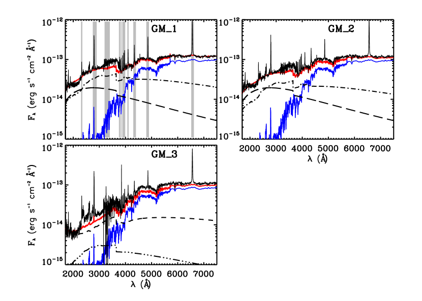
The filling factor of the contributing columns at each epoch is given in Table 2. We list a characteristic value for the energy flux, ${\cal F}_{w}$ , which is an average of the energy flux of all columns, weighted by the filling factor of each column. The listed total filling factor, $f_{total}$ , is the sum of the $f$ values for the contributing columns, providing the total percentage of the surface covered by accretion columns.

The mass accretion rate was found by by adding the contributions of the columns (Ingleby et al., 2013)

\dot{M}=\frac{8\pi R_{\ast}^{2}}{v_{s}^{2}}\sum_{i}{\cal F}_{i}f_{i}=\frac{8\pi R_{\ast}^{2}}{v_{s}^{2}}{\cal F}_{w}f_{total}

(1)

We assume that $v_{s}$ is 0.89 of the free-fall velocity, which for the stellar parameters is 494 ${\rm km\,s^{-1}}$ , corresponding to infall from $\sim$ 5 stellar radii. Values for $\dot{M}$ in the three epochs are given in Table 2. The error in our estimates of the accretion rate is dominated by uncertainties in $A_{V}$ . Existing estimates of extinction for GM Aur range from 0.1 (Kenyon & Hartmann, 1995) to 0.8 (Espaillat et al., 2011) with a value of 0.3 derived from long wavelength optical spectra (Herczeg & Hillenbrand, 2014). We adopted the value listed in Espaillat et al. (2011) in order to directly compare those results to our analysis. The range of measured $A_{V}$ values introduces a factor of 2 error in our $\dot{M}$ estimate.

3.2 FUV to IR variability

Here, we analyze the wavelength dependent variability in the STIS and SpeX data and discuss some of the common contributors to the emission in each spectral region. GM_1 and GM_2, separated by one week, have very similar spectra and in §3.1 we showed that these two epochs had minimal differences in the accretion properties. However, GM_3, which was observed 3 months after GM_1, is clearly dimmer, though the magnitude of the dimming across the spectrum is not uniform (see Figure 1). Namely, the biggest decrease in fluxes occurs in the NUV, with accompanying yet smaller dips in FUV, optical and IR fluxes. In the following analysis we focus on the differences between GM_1 and GM_3.

3.2.1 NUV and optical excess

As shown in Table 2, while the total filling factors for all three epochs are approximately equal, the energy flux of the columns is higher in GM_1 and GM_2 than in GM_3. As a result, the columns in GM_3 emit less in the NUV, significantly lowering the total flux in this wavelength range. This can best be seen in Figure 3, which compares the normalized total flux due to the accretion columns in the three epochs.

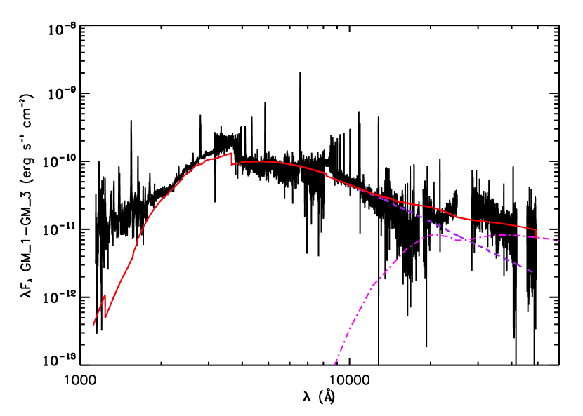
Figure 4 shows the difference in flux between GM_1 and GM_3, with excesses observed in GM_1 at all wavelengths. We fit the NUV and optical portion of this difference spectrum with the emission from an accretion column. We tried fits with columns characterized by log ${\cal F}=10-12$ and found that the best fit to the excess comes from an accretion column with ${\cal F}=3\times 10^{11}$ $erg\;s^{-1}\;cm^{-2}$ and $f$ of 0.006. The accretion rate of a column with these parameters is 5.1 $\times 10^{-9}\;M_{\sun}\,yr^{-1}$ . This $\dot{M}$ is roughly consistent with the difference in $\dot{M}$ between GM_1 and GM_3 listed in Table 2.

To summarize, we find that the difference between the accretion properties of GM_1 and GM_3 is in the energy flux, or density, of the accretion columns rather than the total surface coverage. The decrease of $\dot{M}$ in GM_3 is mainly due to the decreased density in the high density accretion columns.

3.2.2 IR excess

GM Aur is known to be variable in the infrared. Using Spitzer IRS spectra, Espaillat et al. (2011) found a change in the strength of the 10 µm silicate emission and in infrared continuum emission from 5 to 10 µm. They interpreted this as due to changes in the amount of optically thin dust within the disk hole. Espaillat et al. (2011) found that the inner disk hole contained 2 $\times$ 10^-12 M_☉ of optically thin dust and they could reproduce the observed variability by decreasing the amount of dust in the optically thin region by a factor of two.

In Figure 4 we detect an excess in the IR in GM_1 as compared to GM_3. This excess is redder than the emission expected from accretion and therefore not associated with shock emission (Fischer et al., 2011; McClure et al., 2013). We calculated models of optically thin dust emission to fit the SpeX data for GM_1 and GM_3, following the procedure of Espaillat et al. (2010, 2011) to reproduce the excess. The dust is heated by stellar radiation and we change the mass in dust to fit the spectra. The silicate dust composition used in the optically thin region is the same as in Espaillat et al. (2011), which is based on the best fit to the 10 µm silicate feature. We use ISM-sized (0.005–0.25 µm) dust composed of 32 $\%$ organics, 12 $\%$ troilite, and 56 $\%$ silicates. The silicates are 90 $\%$ amorphous and 10 $\%$ crystalline forsterite. We find that to fit the GM_1 spectra we need 1.9 $\times$ 10^-12 M_☉ of dust in the optically thin region, while we need 1.4 $\times$ 10^-12 M_☉ for GM_3. Figure 4 compares the GM_1-GM_3 excess spectrum to the emission from the difference between the two optically thin dust models used to fit the SpeX data.

3.2.3 FUV excess

Figure 4 shows that the observed FUV excess in GM_1 compared to GM_3 cannot be explained by emission from more energetic accretion columns alone. However, it is well known that in addition to shock emission, molecular gas emission contributes to the FUV spectrum, primarily H₂ with a contribution from CO (Herczeg et al., 2002, 2004; Bergin et al., 2004; Ingleby et al., 2009; France et al., 2011a, b). This molecular gas was expected to be within a few AU of the central star, as H₂ was spatially unresolved by Herczeg et al. (2002) for TW Hya, and indeed Ingleby et al. (2011) showed that spectrally resolved H₂ lines originated between the magnetospheric truncation radius, out to $\sim$ 3 AU for the case of RECX 11 in $\eta$ Chameleon.

H₂ in the inner disk is excited via one of two mechanisms. The first is excitation by Ly $\alpha$ photons populating the upper levels of H₂ which then creates a fluorescent spectrum as it de-excites. While Ly $\alpha$ fluorescent lines were identified by Herczeg et al. (2002) in high resolution STIS spectra, the features are detectable at low resolution and are found in the GM Aur FUV spectra for all epochs. The second mechanism is collisional H₂ excitation by free hot electrons. Metals present in the inner disk are ionized by X-rays from the star and these electrons ionize the abundant H and He producing a large supply of hot electrons. Electrons collisionally excite H₂ and therefore different paths for de-excitation are allowed with one path producing continuum emission as the H₂ is dissociated. Therefore the two excitation methods produce unique and distinguishable H₂ emission spectra (Abgrall et al., 1997).

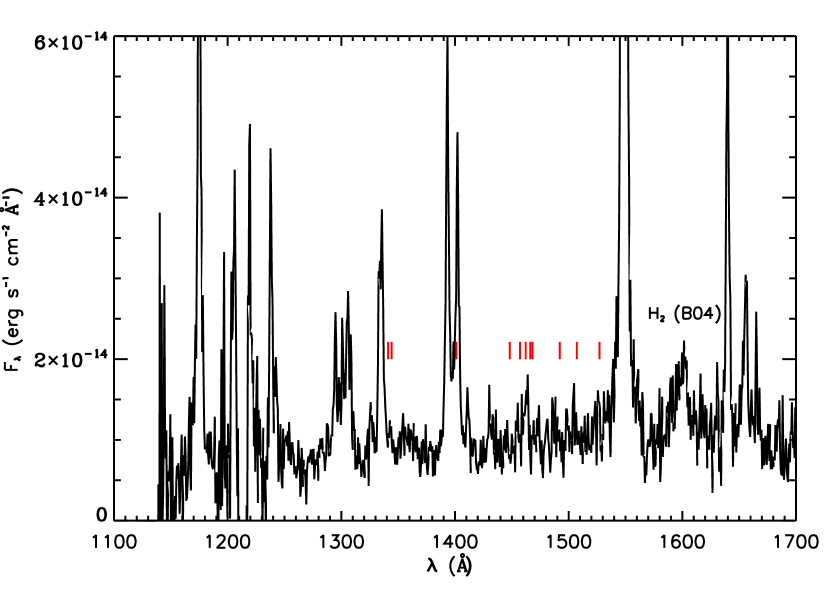
In Figure 5 we show the excess FUV emission after the subtraction of the accretion shock continuum emission (black minus red in Figure 4). The strong FUV atomic lines remain after the removal of the shock, since the accretion shock models do not attempt to produce line emission; however lines such as the Si IV doublet near 1400 Å, C IV at 1548 and 1551 Å and He II $\lambda$ 1640 Å are known to correlate with the mass accretion rate (Johns-Krull et al., 2000; Calvet et al., 2004; Ardila et al., 2013). In addition to the strong hot lines, we see a remaining continuum emission which cannot be explained by the accretion shock. The broad continuum feature at 1600 Å was identified as collisionally excited H₂ emission from the disk of CTTS in Bergin et al. (2004). Ingleby et al. (2009, 2012) showed that this feature is always observed in CTTS but absent in WTTS, when the disk has been dispersed. We observe this continuum feature in the FUV difference spectrum, revealing an excess of collisionally excited H₂ emission coming from the disk in GM_1. Assuming that the difference reflects an increase in H₂ density, we estimate the necessary density difference assuming that the flux in the 1600 Å H₂ feature ( $F_{1600}$ ) is proportional to the H₂ surface density ( $\Sigma_{H_{2}}$ ), or $F_{1600}\propto\Sigma_{H_{2}}^{2}$ (Ingleby et al., 2009). Using this relation, we find that the surface density of H₂ decreased from GM_1 to GM_3 by a factor of 1.4.

The difference spectrum does not support an excess in the Ly $\alpha$ excited H₂ emission. Fluorescent lines easily detected in the original spectra do not appear in Figure 5, indicating that there is little change in this type of H₂ emission when the accretion rate drops. In addition to the observations discussed here, GM Aur was observed with STIS in April, 2003 in GO Program 9374 (PI: E. Bergin) and during August, 2010 in GO Program 11616 (PI: G. Herczeg). The 2010 spectra were analyzed and accretion rates determined in Ingleby et al. (2013) while we calculate $\dot{M}$ for the 2003 data using the method described in §3.1. Accretion rates in 2003 and 2010 were $9.1\times 10^{-9}$ and $9.6\times 10^{-9}$ $M_{\sun}\,yr^{-1}$ , respectively. We compared the fluxes in the strong Ly $\alpha$ fluoresced H₂ lines of all 5 STIS epochs and found that there is no evidence for a correlation with $\dot{M}$ , based on a Pearson r coefficient between 0 and 0.5 for most lines. While Ly $\alpha$ is heavily absorbed by interstellar hydrogen and cannot be observed directly, these results suggest Ly $\alpha$ is not changing between GM_1 and GM_3, contrary to predictions that Ly $\alpha$ is formed in the accretion shock. If instead Ly $\alpha$ is formed in the broad accretion flows, then perhaps the magnetospheric truncation radius is larger when $\dot{M}$ drops, increasing the Ly $\alpha$ emitting region. While interesting, much more substantial work is needed to interpret Ly $\alpha$ in CTTS, for example with efforts to reconstruct the Ly $\alpha$ line profile by observing H₂ fluorescence (Herczeg et al., 2002; Schindhelm et al., 2012).

4 Discussion

In the previous sections, we presented observations which displayed variability in the FUV–NIR emission of GM Aur. From these observations, we extracted four measurements of the properties of GM Aur. First, we measured a lower accretion rate in GM_3 than in GM_1 and GM_2. For GM_3, we also measured a lower dust mass and a lower H₂ density in the inner disk than the earlier GM_1 and GM_2 data. Lastly, the change in the FUV–NIR emission of GM Aur was observed to occur over a timescale of 3 months. In the the following, we consider which physical properties of the system may have been different during GM_3 to explain our observations. In particular, we focus on how inhomogeneities in the inner disk may explain the four measured properties of GM Aur.

We can explain the decrease in the NUV emission of GM Aur with our accretion shock models, which measure a lower accretion rate in GM_3. It is important to define what a single measured accretion rate corresponds to. Accretion rates are derived by measuring the shock emission in excess above the stellar photosphere and using the accretion shock model (or a slab model) to account for the emission outside the observed wavelengths (i.e., $<$ 1000 and $>$ 1 ${\micron}$ in this work). Determining the accretion luminosity from the excess emission, and using the stellar mass and radius, the accretion rate then follows (e.g., Gullbring et al., 1998; Herczeg & Hillenbrand, 2008; Ingleby et al., 2013). And so, the reported accretion rate is a measure of the emission created from mass impacting a region of the stellar surface at a particular point in time, which in turn corresponds to a particular orientation of the star (and hence magnetosphere) and disk along our line of sight. Analysis of the spectral energy distribution of the excess emission in §3.1 indicates that in GM_3 we were observing a magnetospheric region characterized by low density accretion columns. This does not preclude that high density columns were present at other azimuthal regions that were not visible at that time.

Considering 5 epochs of existing STIS spectra (combining the current observations with those obtained in 2003 and 2010), 4 out of 5 times GM Aur was observed during a high state of accretion and in GM_3 we caught it in a low state. Compared to results from accretion shock fitting of our multi-epoch data, the accretion rates in 2003 and 2010 were similar to the higher accretion rates of GM_1 and GM_2 (see $\S$ 3.2.3). Specifically, in the multi-column fitting of the spectra, all but the GM_3 epoch are characterized by high density accretion columns with small filling factors. As discussed in Ingleby et al. (2013), lower density columns could still be contributing, but their emission could not be extracted from the brighter stellar spectrum. Whereas during GM_3 the accretion columns had lower densities with larger stellar surface coverage. Although schematic, this evidence points to an inhomogeneous and variable magnetosphere. This is not surprising given the highly complex nature of the stellar magnetic fields determined by Zeeman Doppler techniques (Donati et al., 2008, 2011, 2013; Gregory & Donati, 2011). However, in addition to the complexity of the magnetic fields, the structure of the inner disk from which the mass is coming from must play a role in the driving the full spectrum of variability.

Simultaneous with the NUV decrease in GM_3, there are decreases in the NIR spectrum and FUV H₂ emission feature at 1600 Å. We attribute these to lower dust masses and lower H₂ densities in the inner disk, respectively. In §3.2.2 we discussed the optically thin dust models used to fit the NIR excess and found that the dust mass was a factor of 1.4 lower in GM_3 than in GM_1. Since the dust is optically thin, this means the dust surface density decreased by a factor of 1.4. Interestingly, 1.4 is the same factor by which we estimate the H₂ density decreased between GM_1 and GM_3 in §3.2.3. This suggests that the H₂ 1600 Å feature is tracing the same location in the disk as the dust, and that the dust and gas are well-mixed in the inner disk. The decrease in the H₂ emission feature at 1600 Å is not accompanied by a change in H₂ fluorescent lines, which should also trace the gas; however, this may be due to different origins of the H₂ lines. As discussed earlier (§3.2.3), the H₂ emission feature at 1600 Å is a consequence of collisional excitation following X-ray ionization of heavy elements in the inner disk (Abgrall et al., 1997; Bergin et al., 2004) while fluorescent lines are due to excitation of electrons to high electronic levels of H₂ by UV Ly $\alpha$ emission (Herczeg et al., 2002). X-rays penetrate deeper into the disk than UV photons because UV radiation is absorbed by small dust grains in the uppermost layers of the disk (Nomura et al., 2007). We expect that the H₂ emission feature at 1600 Å is coming from deeper in the disk and is tracing the same disk regions as seen in the NIR dust emission.

Our analysis suggests a link between the mass in gas and dust in the disk and the mass being loaded onto the star at the magnetospheric truncation radius. However, the kinematic timescales where the gas and dust reside in the disk are problematic given the 3 month time difference between GM_1 and GM_3. At the dust destruction radius, the viscous timescale is $\sim$ 2–10 years using Equation 37 of Hartmann et al. (1998) with R₁ = 10 R_∗, T=5000-1000, and $\alpha$ =0.01. It is unlikely that the mass in the entire inner disk is decreasing within 3 months and that this is causing the lower accretion rate in GM_3 given that the dust and gas in the inner disk are fed by the outer disk on the viscous timescale. A period of 3 months requires a change in the disk to occur near the magnetospheric radius, $\sim$ 5 $R_{\ast}$ . At this radius, the viscous timescale is no longer relevant as material is transported inward along magnetic field lines as opposed to viscously through the disk.

In order for a similar decline of mass in the dust and H₂, the two must be spatially related, but dust must reside outside the dust destruction radius (typically $\sim$ 10 R_∗) where the viscous timescale is much longer than 3 months. However, if we allow large dust grains, 1 mm, and a sublimation temperature of 1600 K (as opposed to the commonly used 1400 K), dust grains can survive down to 0.07 AU, following D’Alessio et al. (2005), which is approximately the corotation radius. Stauffer et al. (2015) found that, for a sample of young stars, IR variability indicates that inner disk walls may be present near the corotation radius. In our simple model, we assume the magnetospheric truncation radius is 5 $R_{\ast}$ (Calvet & Gullbring, 1998), or 0.04 AU. In reality, the truncation radius depends on the strength of the magnetic field and accretion rate. In addition, magnetospheres are complex, therefore the truncation radius varies and may extend to corotation at times (Donati et al., 2011). If some of the NIR emission is produced in the large grains near the midplane (allowing for small grains remaining in the upper layers), then the gas and dust may be co-spatial near the corotation radius and also linked to an extended magnetosphere. Blinova et al. (2015) showed that if the magnetospheric truncation radius ( $r_{m}$ ) is near the corotation radius ( $r_{cor}$ ), $r_{cor}\sim 1.4\;r_{m}$ , then accretion is chaotic and variable, whereas for $r_{cor}>1.4\;r_{m}$ , accretion is stable. Unstable accretion occurs through short lived “tongues”, contributing to inhomogeneous accretion.

While the NUV emission is related to variable accretion, FUV and NIR variability is rooted in the disk. We cannot conclusively say what is leading to inhomogeneities in the inner disk with our low cadence data set. One theory is that disk material builds up near the corotation radius before emptying quickly onto the star (D’Angelo & Spruit, 2012). This would produce a period of lower density in the inner disk after the material is dumped onto the star. While this phenomenon is typically used to describe objects undergoing large accretion bursts (like EXors), D’Angelo & Spruit (2012) note that any object with a strong magnetic field and low accretion rate should undergo this affect at some level. As discussed, the magnetosphere may truncate the disk closer to corotation than typically assumed, and gas and large dust grains may coexist near corotation, linking the decline in disk mass observed with the lower accretion rate. Alternatively, it is possible that inner disk gas may have an emission component in the NIR. Tannirkulam et al. (2008) required the presence of NIR emission inside the dust destruction radius of Herbig Ae stars and suggested optically thick gas as the source. If the NIR does come from inner disk gas, then the inhomogeneities and magnetospheric truncation radius may reside inside corotation.

Another common cause of variability in CTTS stems from variable extinction by dust. GM Aur becomes redder as it dims during the GM_3 epoch and objects with that behavior may be undergoing such variable dust extinction, possibly from warps in the circumstellar disk (Günther et al., 2014; Cody et al., 2014). Variable obscuration requires that the disk be observed close to edge on, as in the well studied case of AA Tau (Bouvier et al., 2013). GM Aur has a well determined inclination of $\sim$ 57^∘ (Dutrey et al., 1998), therefore dust obscuration requires disk structures at large scale heights, unlikely to exist for any sustained period of time. A dimming event in the CTTS RW Aur A (inclined between 45^∘ and 60^∘) may be due to dust carried to large scale heights above the disk in an enhanced wind, producing the obscuration (Petrov et al., 2015); however, RW Aur A is known to have strong outflows as evidenced by existing jets, whereas GM Aur shows no sign of jets. In addition, Ellerbroek et al. (2014) showed that dust lifted to large scale heights above the disk, while producing dimming in the optical by obscuring the star, would increase the NIR emission as the surface area of dust is increased.

In conclusion, we propose that the observations presented here are tracing inhomogeneities in the inner disk and magnetosphere. Parsing out the detailed structure of these regions and how they interact is an extremely difficult task given the high complexity (e.g., Romanova et al., 2008; Kulkarni & Romanova, 2008; Romanova et al., 2012; Kurosawa & Romanova, 2013). In fact, there are some observed properties of GM Aur that we cannot yet explain. We note that while the dust mass and H₂ density decrease by a factor of 1.4 in GM_3, the accretion rate decreases by a factor of 2.8 (although given the errors, these numbers may in fact be more similar). The surface density may not scale exactly with $\dot{M}$ as factors such as temperature and viscosity also play a role. It is puzzling what causes this difference, given that it is not clear exactly how accretion occurs onto the star. In any event, our data connect the disk, near the footprints of the magnetic field lines, to the material in the accretion shock at the stellar surface. Higher cadence observations of GM Aur would be ideal to test our proposal and to make further progress on the issue of variability of TTS.

5 Summary

We analyzed variability in the FUV to NIR spectrum of GM Aur over 3 epochs of observation, separated by one week and 3 months. We found that GM_1 and GM_2 were nearly identical in fluxes. GM_3 was observed during an epoch of low fluxes across the entire spectrum. We drew the following conclusions:

•

The accretion rate of GM_3 was lower than the first two epochs by a factor of 2.8. While the surface coverage of the accretion columns remained approximately constant, the energy flux in the columns decreased in GM_3. Energy flux is related to the density, so GM_3 had low densities in the accretion columns compared to the earlier epochs.
•

We fit SpeX observations, obtained contemporaneously with the STIS spectra, with models of optically thin dust in the inner cavity of GM Aur. During the epoch of low accretion, the mass of dust in the disk decreased by a factor of 1.4.
•

The FUV spectrum indicates that the emission from H₂ molecules decreased during the epoch of low accretion and decreased dust mass. In particular, we found that the spectrum of H₂ collisionally excited by free electrons in the disk described the shape of the excess in GM_1 over GM_3. Moreover, we find that the mass of H₂ changed by the same factor as the dust.
•

GM Aur is seen here to vary within a 3 month period, placing the origin of variability near the magnetospheric truncation radius. If the disk is truncated near corotation and dust can survive near corotation in large grains, then inhomogeneities at that location in the disk can account for accretion variability. The build up and subsequent dumping of material onto the star is one possible explanation for the source of disk inhomogeneities.

We conclude that these FUV-NIR data are providing a glimpse at the complexity of the interaction between the stellar magnetic field and the inner disk. Future observational work is needed to test this conclusion as well as theoretical work on the observable properties of star-disk interactions.

6 Acknowledgments

LI and NC acknowledge support from HST grant No. GO-11608. The authors thank Hal Levinson, Andrew Youdin and Kevin Flaherty for insightful discussions. LI would like to thank the anonymous referee for useful comments and suggestions. The authors acknowledge Daryl Kim for his critical role in the BASS observing program. This work is supported at The Aerospace Corporation by the Independent Research and Development Program.

References

Abgrall et al. (1997) Abgrall, H., Roueff, E., Liu, X., & Shemansky, D. E. 1997, ApJ, 481, 557
Alencar et al. (2010) Alencar, S. H. P., Teixeira, P. S., Guimarães, M. M., et al. 2010, A&A, 519, A88
Andrews et al. (2011) Andrews, S. M., Wilner, D. J., Espaillat, C., et al. 2011, ApJ, 732, 42
Ardila et al. (2013) Ardila, D. R., Herczeg, G. J., Gregory, S. G., et al. 2013, ApJS, 207, 1
Bergin et al. (2004) Bergin, E., Calvet, N., Sitko, M. L., et al. 2004, ApJ, 614, L133
Blinova et al. (2015) Blinova, A. A., Romanova, M. M., & Lovelace, R. V. E. 2015, ArXiv e-prints
Bouvier et al. (2013) Bouvier, J., Grankin, K., Ellerbroek, L. E., Bouy, H., & Barrado, D. 2013, A&A, 557, A77
Bouvier et al. (1999) Bouvier, J., Chelli, A., Allain, S., et al. 1999, A&A, 349, 619
Calvet et al. (2002) Calvet, N., D’Alessio, P., Hartmann, L., et al. 2002, ApJ, 568, 1008
Calvet & Gullbring (1998) Calvet, N., & Gullbring, E. 1998, ApJ, 509, 802
Calvet et al. (2004) Calvet, N., Muzerolle, J., Briceño, C., et al. 2004, AJ, 128, 1294
Calvet et al. (2005) Calvet, N., D’Alessio, P., Watson, D. M., et al. 2005, ApJ, 630, L185
Chen et al. (2006) Chen, C. H., Sargent, B. A., Bohac, C., et al. 2006, ApJS, 166, 351
Chiang & Goldreich (1999) Chiang, E. I., & Goldreich, P. 1999, ApJ, 519, 279
Chou et al. (2013) Chou, M.-Y., Takami, M., Manset, N., et al. 2013, AJ, 145, 108
Cody et al. (2014) Cody, A. M., Stauffer, J., Baglin, A., et al. 2014, AJ, 147, 82
Costigan et al. (2012) Costigan, G., Scholz, A., Stelzer, B., et al. 2012, ArXiv e-prints
Cushing et al. (2004) Cushing, M. C., Vacca, W. D., & Rayner, J. T. 2004, PASP, 116, 362
D’Alessio et al. (2005) D’Alessio, P., Hartmann, L., Calvet, N., et al. 2005, ApJ, 621, 461
D’Angelo & Spruit (2012) D’Angelo, C. R., & Spruit, H. C. 2012, MNRAS, 420, 416
Donati et al. (2008) Donati, J.-F., Jardine, M. M., Gregory, S. G., et al. 2008, MNRAS, 386, 1234
Donati et al. (2011) Donati, J.-F., Bouvier, J., Walter, F. M., et al. 2011, MNRAS, 412, 2454
Donati et al. (2013) Donati, J.-F., Gregory, S. G., Alencar, S. H. P., et al. 2013, MNRAS, 436, 881
Dupree et al. (2014) Dupree, A. K., Brickhouse, N. S., Cranmer, S. R., et al. 2014, ApJ, 789, 27
Dutrey et al. (1998) Dutrey, A., Guilloteau, S., Prato, L., et al. 1998, A&A, 338, L63
Edwards et al. (2006) Edwards, S., Fischer, W., Hillenbrand, L., & Kwan, J. 2006, ApJ, 646, 319
Ellerbroek et al. (2014) Ellerbroek, L. E., Podio, L., Dougados, C., et al. 2014, A&A, 563, A87
Espaillat et al. (2007) Espaillat, C., Calvet, N., D’Alessio, P., et al. 2007, ApJ, 670, L135
Espaillat et al. (2011) Espaillat, C., Furlan, E., D’Alessio, P., et al. 2011, ApJ, 728, 49
Espaillat et al. (2010) Espaillat, C., D’Alessio, P., Hernández, J., et al. 2010, ApJ, 717, 441
Espaillat et al. (2014) Espaillat, C., Muzerolle, J., Najita, J., et al. 2014, ArXiv e-prints
Fischer et al. (2011) Fischer, W., Edwards, S., Hillenbrand, L., & Kwan, J. 2011, ApJ, 730, 73
France et al. (2011a) France, K., Yang, H., & Linsky, J. L. 2011a, ApJ, 729, 7
France et al. (2011b) France, K., Schindhelm, E., Burgh, E. B., et al. 2011b, ApJ, 734, 31
Gregory & Donati (2011) Gregory, S. G., & Donati, J.-F. 2011, Astronomische Nachrichten, 332, 1027
Gullbring et al. (1998) Gullbring, E., Hartmann, L., Briceno, C., & Calvet, N. 1998, ApJ, 492, 323
Günther et al. (2014) Günther, H. M., Cody, A. M., Covey, K. R., et al. 2014, AJ, 148, 122
Hartigan et al. (1991) Hartigan, P., Kenyon, S. J., Hartmann, L., et al. 1991, ApJ, 382, 617
Hartmann et al. (1998) Hartmann, L., Calvet, N., Gullbring, E., & D’Alessio, P. 1998, ApJ, 495, 385
Herbst et al. (1994) Herbst, W., Herbst, D. K., Grossman, E. J., & Weinstein, D. 1994, AJ, 108, 1906
Herczeg & Hillenbrand (2008) Herczeg, G. J., & Hillenbrand, L. A. 2008, ApJ, 681, 594
Herczeg & Hillenbrand (2014) —. 2014, ApJ, 786, 97
Herczeg et al. (2002) Herczeg, G. J., Linsky, J. L., Valenti, J. A., Johns-Krull, C. M., & Wood, B. E. 2002, ApJ, 572, 310
Herczeg et al. (2004) Herczeg, G. J., Wood, B. E., Linsky, J. L., Valenti, J. A., & Johns-Krull, C. M. 2004, ApJ, 607, 369
Hughes et al. (2009) Hughes, A. M., Andrews, S. M., Espaillat, C., et al. 2009, ApJ, 698, 131
Ingleby et al. (2012) Ingleby, L., Calvet, N., Herczeg, G., & Briceño, C. 2012, ApJ, 752, L20
Ingleby et al. (2009) Ingleby, L., Calvet, N., Bergin, E., et al. 2009, ApJ, 703, L137
Ingleby et al. (2011) —. 2011, ApJ, 743, 105
Ingleby et al. (2013) Ingleby, L., Calvet, N., Herczeg, G., et al. 2013, ApJ, 767, 112
Johns-Krull et al. (2000) Johns-Krull, C. M., Valenti, J. A., & Linsky, J. L. 2000, ApJ, 539, 815
Kenyon & Hartmann (1995) Kenyon, S. J., & Hartmann, L. 1995, ApJS, 101, 117
Koenigl (1991) Koenigl, A. 1991, ApJ, 370, L39
Koerner et al. (1993) Koerner, D. W., Sargent, A. I., & Beckwith, S. V. W. 1993, Icarus, 106, 2
Kulkarni & Romanova (2008) Kulkarni, A. K., & Romanova, M. M. 2008, MNRAS, 386, 673
Kurosawa & Romanova (2013) Kurosawa, R., & Romanova, M. M. 2013, MNRAS, 431, 2673
Long et al. (2008) Long, M., Romanova, M. M., & Lovelace, R. V. E. 2008, MNRAS, 386, 1274
Manara et al. (2014) Manara, C. F., Testi, L., Natta, A., et al. 2014, ArXiv e-prints
Marsh & Mahoney (1992) Marsh, K. A., & Mahoney, M. J. 1992, ApJ, 395, L115
Matthews et al. (2014) Matthews, B. C., Krivov, A. V., Wyatt, M. C., Bryden, G., & Eiroa, C. 2014, Protostars and Planets VI
McClure et al. (2013) McClure, M. K., Calvet, N., Espaillat, C., et al. 2013, ApJ, 769, 73
Micela & Marino (2003) Micela, G., & Marino, A. 2003, A&A, 404, 637
Morales-Calderón et al. (2011) Morales-Calderón, M., Stauffer, J. R., Hillenbrand, L. A., et al. 2011, ApJ, 733, 50
Nomura et al. (2007) Nomura, H., Aikawa, Y., Tsujimoto, M., Nakagawa, Y., & Millar, T. J. 2007, ApJ, 661, 334
Owen et al. (2012) Owen, J. E., Clarke, C. J., & Ercolano, B. 2012, MNRAS, 422, 1880
Owen et al. (2010) Owen, J. E., Ercolano, B., Clarke, C. J., & Alexander, R. D. 2010, MNRAS, 401, 1415
Petrov et al. (2015) Petrov, P. P., Gahm, G. F., Djupvik, A. A., et al. 2015, ArXiv e-prints
Rayner et al. (2003) Rayner, J. T., Toomey, D. W., Onaka, P. M., et al. 2003, PASP, 115, 362
Rice et al. (2003) Rice, W. K. M., Wood, K., Armitage, P. J., Whitney, B. A., & Bjorkman, J. E. 2003, MNRAS, 342, 79
Rigliaco et al. (2011) Rigliaco, E., Natta, A., Randich, S., Testi, L., & Biazzo, K. 2011, A&A, 525, A47
Romanova et al. (2008) Romanova, M. M., Kulkarni, A. K., & Lovelace, R. V. E. 2008, ApJ, 673, L171
Romanova et al. (2012) Romanova, M. M., Ustyugova, G. V., Koldoba, A. V., & Lovelace, R. V. E. 2012, MNRAS, 421, 63
Schindhelm et al. (2012) Schindhelm, E., France, K., Burgh, E. B., et al. 2012, ApJ, 746, 97
Shu et al. (1994) Shu, F., Najita, J., Ostriker, E., et al. 1994, ApJ, 429, 781
Siess et al. (2000) Siess, L., Dufour, E., & Forestini, M. 2000, A&A, 358, 593
Skrutskie et al. (1990) Skrutskie, M. F., Dutkevitch, D., Strom, S. E., et al. 1990, AJ, 99, 1187
Stauffer et al. (2014) Stauffer, J., Cody, A. M., Baglin, A., et al. 2014, AJ, 147, 83
Stauffer et al. (2015) Stauffer, J., Cody, A. M., McGinnis, P., et al. 2015, ArXiv e-prints
Strom et al. (1989) Strom, K. M., Strom, S. E., Edwards, S., Cabrit, S., & Skrutskie, M. F. 1989, AJ, 97, 1451
Tannirkulam et al. (2008) Tannirkulam, A., Monnier, J. D., Millan-Gabet, R., et al. 2008, ApJ, 677, L51
Uchida & Shibata (1985) Uchida, Y., & Shibata, K. 1985, PASJ, 37, 515
Vacca et al. (2003) Vacca, W. D., Cushing, M. C., & Rayner, J. T. 2003, PASP, 115, 389
Whittet et al. (2004) Whittet, D. C. B., Shenoy, S. S., Clayton, G. C., & Gordon, K. D. 2004, ApJ, 602, 291
Wolk et al. (2005) Wolk, S. J., Harnden, Jr., F. R., Flaccomio, E., et al. 2005, ApJS, 160, 423
Zhu et al. (2011) Zhu, Z., Nelson, R. P., Hartmann, L., Espaillat, C., & Calvet, N. 2011, ApJ, 729, 47
Zuckerman (2001) Zuckerman, B. 2001, ARA&A, 39, 549

Table 1: Log of Observations

Epoch	Telescope/ Instrument	Date of Obs
GM_1	HST/STIS	09-11-2011
GM_1	IRTF/SpeX	09-11-2011
GM_2	HST/STIS	09-17-2011
GM_2	IRTF/SpeX	09-18-2011
GM_3	HST/STIS	01-05-2012
GM_3	IRTF/SpeX	01-06-2012

Table 2: Results from Multi-Component Model Fits to UV and Optical Spectra

Object	$f(3\times 10^{10})$	$f(10^{11})$	$f(3\times 10^{11})$	$f(10^{12})$	$f_{total}$	Weighted ${\cal F}$	$\dot{M}\;(M_{\sun}\,yr^{-1})$
GM_1	0	0.03	0	0.001	0.031	$1.3\times 10^{11}$	$1.1\times 10^{-8}$
GM_2	0	0.02	0	0.001	0.021	$1.4\times 10^{11}$	$8.5\times 10^{-9}$
GM_3	0.04	0	0.0006	0	0.041	$3.4\times 10^{10}$	$3.9\times 10^{-9}$

Note. — The values in parentheses represents the energy flux ( ${\cal F}$ ) of each column in erg s^-1 cm^-3.