Modal and nonmodal stability analysis of electrohydrodynamic flow with and without cross-flow

Abstract

We report the results of a complete modal and nonmodal linear stability analysis of the electrohydrodynamic flow (EHD) for the problem of electroconvection in the strong injection region. Convective cells are formed by Coulomb force in an insulating liquid residing between two plane electrodes subject to unipolar injection. Besides pure electroconvection, we also consider the case where a cross-flow is present, generated by a streamwise pressure gradient, in the form of a laminar Poiseuille flow. The effect of charge diffusion, often neglected in previous linear stability analyses, is included in the present study and a transient growth analysis, rarely considered in EHD, is carried out. In the case without cross-flow, a non-zero charge diffusion leads to a lower linear stability threshold and thus to a more unstable flow. The transient growth, though enhanced by increasing charge diffusion, remains small and hence cannot fully account for the discrepancy of the linear stability threshold between theoretical and experimental results. When a cross-flow is present, increasing the strength of the electric field in the high-$Re$ Poiseuille flow yields a more unstable flow in both modal and nonmodal stability analyses. Even though the energy analysis and the input-output analysis both indicate that the energy growth directly related to the electric field is small, the electric effect enhances the lift-up mechanism. The symmetry of channel flow with respect to the centerline is broken due to the additional electric field acting in the wall-normal direction. As a result, the centers of the streamwise rolls are shifted towards the injector electrode, and the optimal spanwise wavenumber achieving maximum transient energy growth increases with the strength of the electric field.

1 Introduction

1.1 General description of EHD flow

Electrohydrodynamics (EHD) is concerned with the interaction between an electric field and a flow field. Such configurations have broad applications in a range of industrial and biological devices. EHD effects can be used to enhance the heat transfer efficiency (Jones, 1978; Allen & Karayiannis, 1995), to design microscale electrohydrodynamic pumps (Bart et al., 1990; Darabi et al., 2002), to fabricate diagnostic devices and drug delivery systems (Chakraborty et al., 2009) and DNA microarrays (Lee et al., 2006), and to design new strategies for active flow control (Bushnell & McGinley, 1989). Physically, EHD flow is characterized by a strong nonlinear interaction between the velocity field, the electric field and space charges: the electric force results in flow motion, which in turn affects the charge transport. The intricate nature of this nonlinearity defies a fundamental understanding of EHD flow. Moreover, as we will see, there still remains a mismatch or discrepancy between experimental observations and a theoretical analysis.

One classic problem in EHD, named electroconvection, deals with the convective motions induced by unipolar charge injection into a dielectric liquid (of very low conductivity) which fills the gap between two parallel rigid plane electrodes. The Coulomb force acting on the free charge carriers tends to destabilize the system. Electroconvection is often compared to Rayleigh-Bénard convection (RBC) because of their similar geometry and convection patterns. Moreover, RBC is known to be analogous to the Taylor-Couette (TC) flow in the gap between two concentric rotating cylinders, where thermal energy transport in RBC corresponds to the transport of angular momentum in TC flow (Bradshaw, 1969; Grossmann & Lohse, 2000). In the linear regime of RBC, the flow is destabilized by the buoyancy force caused by the continued heating of the lower wall (an analogous role is played by centrifugal force in TC flow). As the thermal gradient exceeds a critical value, chaotic motion sets in. In EHD flow, the destabilizing factor is the electric force, acting in the wall-normal direction. However, the analogy between the two flows ends, as soon as nonlinearities arise, especially as diffusive effects are concerned: in RBC, molecular diffusion constitutes the principal dissipative mechanism whereas in EHD flow, it is the ion drift velocity $KE$ (with $K$ being the ionic mobility) which diffuses perturbations in the fluid. It is well-known that RBC is of a supercritical nature, i.e., transition from the hydrostatic state to the finite-amplitude state occurs continuously as the controlling parameter, i.e., the Rayleigh number, is increased. For EHD flow, on the other hand, the bifurcation is subcritical, characterized (i) by an abrupt jump in motion amplitude from zero to a finite value, as a critical parameter is crossed, and (ii) by the existence of a hysteresis loop. It is interesting to mention an analogy between EHD flow and polymeric flow: polymeric flow shows a hysteresis loop as well, as the first bifurcation is considered. In fact, the counterpart of EHD flow, i.e., magneto-hydrodynamics (MHD) flow, has been compared to polymeric flow in Ogilvie & Proctor (2003).

Most studies in the EHD literature address electroconvection in the hydrostatic condition, i.e., without cross-flow. In this work we also investigate the EHD stability properties in the presence of cross-flow. Our interest is two-fold. First, the potential of this flow configuration resides in the possibility of using the electric field to create large-scale rollers for flow manipulation; turbulent drag reduction designed in the spirit of Schoppa & Hussain (1998) and investigated by Soldati & Banerjee (1998) in the nonlinear regime is an example of this type. Secondly, EHD with cross-flow has been applied to wire-plate electrostatic precipitators, but due to the complex nature of the chaotic interaction between wall turbulence and the electric field, our current understanding of such flows is rather limited. Nonlinear EHD simulations with a cross-flow component have been reported in Soldati & Banerjee (1998). More relevant to our linear problem is the unipolar-injection-induced instabilities in plane parallel flows studied by Atten & Honda (1982) and Castellanos & Agrait (1992). The former work focused on so-called electroviscous effects, defined by an increase of viscosity due to the applied electric field compared to the canonical channel flow. The latter work found that, at high Reynolds numbers, the destabilizing mechanism is linked to inertia, while, at sufficiently low Reynolds numbers, EHD instability are dominant. In this article, we will not only address the modal stability problem of EHD channel flow, as those two previous studies did, we will also take into account transient effects, discussed shortly below, of the high-$Re$ number channel flow in the presence of an electric field. Our results would be interesting to the researchers in the flow instability and transition to turbulence, especially for high-$Re$ flow. The results will also shed light on the study of flow control strategy using EHD effects.

1.2 Stability of EHD flow

The endeavor to understand the stability and transition to turbulence in EHD flow dates back to the 1970’s, when Schneider & Watson (1970) and Atten & Moreau (1972), among the first, performed a linear stability analysis on the flow of dielectric liquids confined between two parallel electrodes with unipolar injection of charges. The mechanism for linear instability could be explained via the formation of an electric torque engendered by the convective motion when the driving electric force is sufficiently strong to overcome viscous diffusion. It was established in Atten & Moreau (1972) that, in the weak injection limit, $C\ll 1$, with $C$ as the charge injection level, the flow is characterized by the criterion $T_{c}C^{2}\approx 220.7$, where $T_{c}$ is the linear stability criterion for the stability parameter $T$, defined in the mathematical modeling section 2.2, and, in the case of space-charge-limited (SCL) injection, $C\rightarrow\infty$, they found $T_{c}\approx 160.75$. However, according to Lacroix et al. (1975) and Atten & Lacroix (1979), the experimentally determined stability criterion was notably different from the theoretical calculations. In the experiments performed by Atten & Lacroix (1979), the linear criterion was found to be $T_{c}\approx 100$ in the case of SCL, which is far lower than the theoretically predicted value. It was argued then that this disagreement might be due to neglecting charge diffusion (Atten, 1976). We will address this discrepancy in the SCL in this paper, and confirm that charge diffusion is indeed an important factor influencing the linear stability criterion in this case.

The first nonlinear stability analysis was performed by Félici (1971), who assumed a two-dimensional, a priori hydraulic model for the velocity field in the case of weak injection between two parallel plates. It was found that within the interval $[T_{nl},T_{c}]$, where $T_{nl}$ is the nonlinear stability criterion for $T$, two solutions exist, namely, a stable state and an unstable finite-amplitude state. This finding corroborated the fact that the bifurcation in the unipolar injection problem is of a subcritical nature and that the flow has a hysteresis loop, as experimentally verified by Atten & Lacroix (1979). Physically, this subcritical bifurcation is related to the formation of a region of zero charge (Pérez & Castellanos, 1989). Later, this simple hydraulic model was extended to three-dimensional, hexagonal convective cells for the case of SCL by Atten & Lacroix (1979), and it was shown that the most unstable hydrodynamic mode consists of hexagonal cells with the interior liquids flowing towards the injector. The nonlinear stability criterion for three-dimensional, hexagonal cells, according to Atten & Lacroix (1979), was $T_{nl}\approx 90$ in the experiments, but theoretical studies produced $T_{nl}\approx 110$.

Most of the previous linear stability analyses of EHD flow focus on the most unstable mode of the linear system, which is insufficient for a comprehensive flow analysis. In fact, theoretically, the linear stability analysis is linked to the characteristics of the linearized Navier-Stokes (N-S) operator $\bm{\mathcal{L}}$ which, in the case of shear flows (in this paper, the cross-flow case), may be highly nonnormal, i.e., $\bm{\mathcal{L}}^{+}\bm{\mathcal{L}}\neq\bm{\mathcal{L}}\bm{\mathcal{L}}^{+}$ (with $\bm{\mathcal{L}}^{+}$ denoting the adjoint of $\bm{\mathcal{L}}$) or, expressed differently, the eigenvectors of the linear operator are mutually nonorthogonal (see Trefethen et al., 1993; Schmid & Henningson, 2001). For a normal operator ($\bm{\mathcal{L}}^{+}\bm{\mathcal{L}}=\bm{\mathcal{L}}\bm{\mathcal{L}}^{+}$), the dynamics of the perturbations is governed by the most unstable mode over the entire time horizon. In contrast, a nonnormal operator has the potential for large transient amplification of the disturbance energy in the early linear phase, even though the most unstable mode is stable. The theory of nonmodal stability analysis (Farrell & Ioannou, 1996; Schmid, 2007), the main tool to be used in this work, has been applied successfully to explain processes active during transition to turbulence in several shear flows. The fact that the bifurcation of EHD flow is subcritical, a trait often observed in shear flows governed by nonnormal linearized operators, tempts one to think that the discrepancy between the experimental value $T_{c}\approx 100$ and the theoretical value $T_{c}\approx 161$ in the SCL regime of EHD flow might be examined in the light of nonmodal stability theory. In fact, it seems surprising that this type of stability analysis has so far only rarely been applied to EHD flows, except for the work of Atten (1974) in the case of hydrostatic flow. The method we employ here is different from Atten’s quasistationary approach: nonmodal stability theory, based on solving the initial-value problem, seeks the maximum disturbance energy growth over entire time horizon when considering all admissible initial conditions and identifies the optimal initial condition for achieving this maximum energy growth. In Atten (1974), a quasistationary approach was taken that proposed that disturbances grow rapidly, compared to the time variation of the thickness of the unipolar layer; however, transient energy growth due to the nonnormality of the linearized operator in hydrostatic EHD has been found to be rather limited in this work. This is in contrast with EHD Poiseuille flow, where nonnormality is prevalent and should be considered from the outset.

The present paper extends the work by Martinelli et al. (2011) and is organized as follows. In § 2, we present the mathematical model, the governing equations and the framework of the linear stability analysis. In § 3, numerical details are given and a code validation is provided in the appendix. We then present in § 4 the results of the modal and nonmodal stability analysis and in § 5 the energy analysis. Finally, in § 6, we summarize our findings and conclude with a discussion.

2 Problem formulation

2.1 Mathematical modeling

We consider the planar geometry sketched in figure 1, where the Cartesian coordinate system used in this work is ($x$, $y$, $z$) or ($\bm{1}_{x}$, $\bm{1}_{y}$, $\bm{1}_{z}$) as the streamwise, wall-normal and spanwise directions, respectively. The two flat electrodes extend infinitely in the $x$- and $z$-directions, and the applied voltage only varies in the $y$-direction. The distance between the two electrodes is $2L^{*}$. The dimensional variables and parameters are denoted with a superscript ^∗.

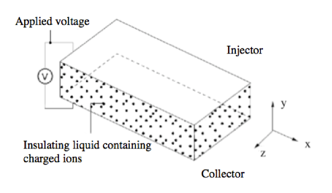
Figure 1: Sketch of the electroconvection problem with coordinate system ($x$, $y$, $z$). In the non-hydrostatic case, a flow rate is induced along the streamwise ($x$) direction.

The electric field satisfies the reduced Maxwell equations. The charges are generated through electrochemical reactions on the charge-injecting electrode (Alj et al., 1985). Since the electric conductivity is very low, conduction currents are negligible even in the presence of large electric fields. Therefore, magnetic effects in the Maxwell equations can be neglected (Melcher, 1981; Castellanos, 1998), leading to the quasi-electrostatic limit of the Maxwell equations ∇^* ×E^* &=0,
∇^* ⋅D^* =Q^*,
∂Q*∂t* + ∇^* ⋅J^* =0, where $\bm{E}^{*}$ is the electric field, $\bm{D}^{*}=\epsilon^{*}\bm{E}^{*}$ denotes the electric displacement, $\epsilon^{*}$ stands for the fluid permittivity which we assume constant here, $Q^{*}$ represents the charge density and $\bm{J}^{*}$ is the current density. Considering equation (1a), it is a well-known practice to define a potential field $\phi^{*}$ according to $\bm{E}^{*}=-\bm{\nabla}^{*}\phi^{*}$. Combining the first two equations (1a) and (1b), we can write the governing equation for $\phi^{*}$ as

$$\nabla^{*2}\phi^{*}=-\frac{Q^{*}}{\epsilon^{*}}.$$ (1)

The current density $\bm{J}^{*}$ arises from several sources. By modeling the EHD flow with only one ionic species in a perfectly insulating fluid (conductivity $\sigma^{*}=0$), one can express $\bm{J}^{*}$ as (Castellanos, 1998)

$$\bm{J}^{*}=K^{*}\bm{E}^{*}Q^{*}+\bm{U}^{*}Q^{*}-D^{*}_{\nu}\bm{\nabla}^{*}Q^{*}$$ (2)

where the first term accounts for the drift of ions (with respect to the fluid) under the effect of the electric field, moving at the relative velocity $K^{*}\bm{E}^{*}$, with $K^{*}$ as the ionic mobility, the second term represents the convection of ions due to the fluid velocity $\bm{U}^{*}$, and the last term takes into account the charge diffusion, with $D^{*}_{\nu}$ as the diffusion coefficient. Since the work of Pérez & Castellanos (1989), the vast body of literature, with the exception of Kourmatzis & Shrimpton (2012) for turbulent EHD flow, neglects the charge-diffusion term because of its small value when compared to the drift terms. However, we will show that, even though the numerical value of $D^{*}_{\nu}$ is very small, its impact on the flow dynamics is undeniable.

The flow field is incompressible, viscous and Newtonian and governed by the Navier-Stokes equations, which, in vector notation, read ∇^* ⋅U^*&=0,
ρ^* ∂U*∂t* + ρ^* ( U^* ⋅∇^*) U^*=-∇^* P^* + μ^* ∇^*2 U^*+ F_q^* , where $\bm{U}^{*}$ is the velocity field, $P^{*}$ the pressure, $\rho^{*}$ the density, $\mu^{*}=\rho^{*}\nu^{*}$ the dynamic viscosity ($\nu^{*}$ the kinematic viscosity) and $\bm{F_{q}}^{*}$ the volumic density of electric force, which expresses the coupling between the fluid and the electric field. In general, $\bm{F_{q}}^{*}$ can be written as

$$\bm{F_{q}}^{*}=Q^{*}\bm{E}^{*}-\frac{1}{2}|\bm{E}^{*}|^{2}\bm{\nabla}^{*}\epsilon^{*}+\bm{\nabla}^{*}\Big{[}\frac{|\bm{E}^{*}|^{2}}{2}\rho^{*}\frac{\partial\epsilon^{*}}{\partial\rho^{*}}\Big{]},$$ (3)

where the three terms on the right-hand side represent, respectively, the Coulomb force, the dielectric force and the electrostrictive force. The Coulomb force is commonly the strongest force when a DC voltage is applied. As we assume an isothermal and homogeneous fluid, the permittivity $\epsilon$ is constant in space. As a result, the dielectric force is zero (however, it would be dominant in the case of an AC voltage). The electrostrictive force can be incorporated into the pressure term of the Navier-Stokes equation as it can be expressed as the gradient of a scalar field. Therefore, the only remaining term of interest in our formulation is the Coulomb force.

The system is supplemented by suitable boundary conditions. In our problem, we assume periodic boundary conditions in the wall-parallel directions. The no-slip and no-penetration conditions for the velocities are assumed at the channel walls. For the potential field, we require Dirichlet conditions on both walls, on the injector $\phi^{*}(L^{*})=\phi^{*}_{0}$ and the collector $\phi^{*}(-L^{*})=0$ in order to fix the potential drop $\Delta\phi_{0}^{*}$ between the electrodes. The injection mechanism is autonomous and homogeneous, meaning that the charge density is constant on the injector, not influenced by the nearby electric field and has a zero wall-normal flux of charge on the collector, i.e., $Q^{*}(L^{*})=-Q^{*}_{0}$ and $\frac{\partial Q^{*}}{\partial y^{*}}(-L^{*})=0$. Owing to the homogeneity in the wall-parallel directions, there is no requirement for boundary conditions in the $x$- and $z$-direction.

2.2 Nondimensionalized governing equations

In the no-crossflow case, as we are interested in the effect of the electric field on the flow dynamics, we nondimensionalize the full system with the characteristics of the electric field, i.e., $L^{*}$ (half distance between the electrodes), $\Delta\phi_{0}^{*}$ (voltage difference applied to the electrodes) and $Q^{*}_{0}$ (injected charge density). Accordingly, the time $t^{*}$ is nondimensionalized by $L^{*2}/(K^{*}\Delta\phi_{0}^{*})$, the velocity $\bm{U}^{*}$ by $K^{*}\Delta\phi_{0}^{*}/L^{*}$, the pressure $P^{*}$ by $\rho^{*}_{0}K^{*2}\Delta\phi_{0}^{*2}/L^{*2}$, the electric field $\bm{E}^{*}$ by $\Delta\phi_{0}^{*}/L^{*}$ and the electric density $Q^{*}$ by $Q^{*}_{0}$. Therefore, the nondimensional equations read ∇⋅U&= 0,
∂U∂t + ( U ⋅∇) U = -∇ P + M2T ∇^2 U+ CM^2 QE,
∂Q∂t + ∇ ⋅[(E+ U)Q] = 1Fe∇^2 Q,
∇^2 ϕ= -CQ,
E = -∇ ϕ where

$$M=\frac{(\epsilon^{*}/\rho^{*}_{0})^{\frac{1}{2}}}{K^{*}},\qquad T=\frac{\epsilon^{*}\Delta\phi_{0}^{*}}{K^{*}\mu^{*}},\qquad C=\frac{Q_{0}^{*}L^{*2}}{\Delta\phi^{*}_{0}\epsilon^{*}},\qquad Fe=\frac{K^{*}\Delta\phi^{*}_{0}}{D_{\nu}^{*}}.$$ (4)

Additionally, the nondimensional boundary conditions are $\bm{U}(\pm 1)=0$, $\phi(1)=1$, $\phi(-1)=0$, $Q(1)=-1$ and $\frac{\partial Q}{\partial y}(-1)=0$.

Various dimensionless groups appear in the equations as written above. $M$ is the ratio between the hydrodynamic mobility $(\epsilon/\rho_{0})^{\frac{1}{2}}$ and the true ion mobility $K$. Gases usually take on a value of $M$ less than $0.1$ and liquids have values of $M$ greater than $1$ (Castellanos & Agrait, 1992). $T$ (Taylor’s parameter) represents the ratio of the Coulomb force to the viscous force. It is the principal stability parameter, assuming a similar role as the Rayleigh number in Rayleigh-Bénard convection. $C$ measures the injection level. When $C\gg 1$, the system is in a strong-injection regime, and when $C\ll 1,$ it is in a weak-injection regime. $Fe$ is the reciprocal of the charge diffusivity coefficient. The factor ${M^{2}}/{T}$ appearing in equation (2.2b) can be interpreted as the ratio between the charge relaxation time $L^{*2}/(K^{*}\Delta\phi^{*}_{0})$ by drift and the momentum relaxation time $L^{*2}/\nu^{*}$. This mathematical model for EHD flow has been assumed and studied in many previous investigations of the linear stability and turbulence analyses for a dielectric liquid subject to unipolar injection of ions (Lacroix et al., 1975; Traoré & Pérez, 2012; Wu et al., 2013), except that the diffusion term in equation (2.2c) is usually neglected (excluding the study of Kourmatzis & Shrimpton (2012)).

2.3 Linear stability problem

The linear problem is obtained by decomposing the flow variable as a sum of base state and perturbation, i.e., $\bm{U}=\bar{\bm{U}}+\bm{u}$, $P=\bar{P}+p$, $\bm{E}=\bar{\bm{E}}+\bm{e}$, $\bm{D}=\bar{\bm{D}}+\bm{d}$, $Q=\bar{Q}+q$ and $\phi=\bar{\phi}+\varphi$. For the vector fields, we have $\bm{u}=(u,v,w)$ and $\bm{e}=(e_{1},e_{2},e_{3})$ along the three Cartesian coordinate directions. After substituting the decompositions into the governing equations (2.2a-e), subtracting from them the governing equations for the base states and retaining the terms of first order, the linear system reads ∇ ⋅u &= 0,
∂u∂t + (u ⋅∇) ¯U + (¯U ⋅∇) u = -∇ p + M2T ∇^2 u+ CM^2 (q¯E+¯Qe),
∂q∂t + ∇ ⋅[(¯E+ ¯U)q +(e+ u)¯Q ] = 1Fe∇^2 q,
∇^2 φ= -Cq,
e = -∇ φ, with the boundary conditions for the fluctuations $\bm{u}(\pm 1)=0$, $\varphi(\pm 1)=0$ and $q(1)=0,\frac{\partial q}{\partial y}(-1)=0$.

2.3.1 Base states

The base states are the solutions to equations (2.2a-e) in the case of no time dependence. Owing to the periodicity in the wall-parallel directions, we can reduce the shape of the base states as functions of $y$ only, that is, $\bar{\bm{U}}=\bar{U}(y)\bm{1}_{y}$ and $\bar{\bm{E}}=\bar{E}(y)\bm{1}_{y}$. For the base flow $\bar{U}(y)$, we are interested in the hydrostatic and pressure-driven Poiseuille flows which, after nondimensionalization, are given by

$$\bar{U}(y)=0,\qquad\qquad\bar{U}(y)=Re\frac{M^{2}}{T}(1-y^{2})=(1-y^{2}),$$ (5)

respectively, in which the (electric) Reynolds number is defined as $Re=\frac{T}{M^{2}}=K^{*}\Delta\phi^{*}_{0}/\nu^{*}$ (in order to enforce the same constant flow rate). It is a passive parameter in the hydrostatic case, but becomes a free parameter in the presence of high-$Re$ cross-flow, in which, consequently, $M$ would be the passive parameter. Therefore, in the Poiseuille flow case, we modify the governing equation (2.3b) by substituting the relation $Re=T/M^{2}$ to obtain

$$\frac{\partial\bm{u}}{\partial t}+(\bm{u}\cdot\bm{\nabla})\bar{\bm{U}}+(\bar{\bm{U}}\cdot\bm{\nabla})\bm{u}=-\bm{\nabla}p+\frac{1}{Re}\nabla^{2}\bm{u}+\frac{CT}{Re}(q\bar{\bm{E}}+\bar{Q}\bm{e}).$$ (6)

By doing so, it is more obvious to identify the effects of $T$ and $C$ on the electric force term. The parameter $Re=K^{*}\Delta\phi^{*}_{0}/\nu^{*}$ here coincides with the canonical hydrodynamic equivalent $Re_{h}=U^{*}L^{*}/\nu^{*}$ because of the electric scaling we chose. However, in a general sense, the two may not necessarily be identical. The nondimensional quantity

$$\frac{Re}{Re_{h}}=\frac{K^{*}\Delta\phi^{*}_{0}}{U^{*}L^{*}}=\frac{L^{*}/U^{*}}{L^{*2}/(K^{*}\Delta\phi^{*}_{0})}$$ (7)

relates the eddy turn-over time and the charge relaxation time by the drift. According to the equality $T=Re\cdot M^{2}$, when $Re$ is near linear criticality at $5772$ and $T$ is around $10^{2}$, $M\approx 0.1$. It implies that the working liquid is gas. Moreover, in contrast to the nonlinear constitutive modeling for polymers in viscoelastic flow, the base flow is not modified under the influence of the base electric field, even though the coupling between $\bm{U}$ and $Q$ is nonlinear in equation (2.2c). This is because the directions of the base flow and the base electric field are perpendicular. Nevertheless, the base pressure gradient in the wall-normal direction is no longer zero.

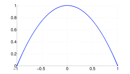
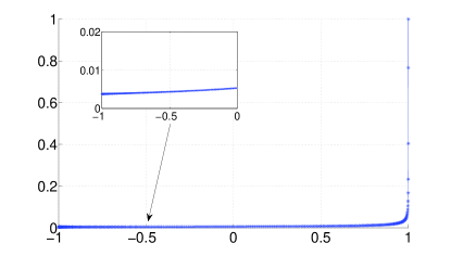
Figure 2: The base states: (a) $\bar{U}$, (b) $\bar{\phi}$, (c) $\bar{Q}$.

The base electric field $\bar{\bm{E}}(y)$ can be solved from equations (2.2c-e), recast into an equation only for $\bar{\phi}$ which reads

$$\bar{\phi}^{\prime}\bar{\phi}^{\prime\prime\prime}+(\bar{\phi}^{\prime\prime})^{2}+\frac{1}{Fe}\bar{\phi}^{\prime\prime\prime\prime}=0,$$ (8)

where prime ^′ denotes the spatial derivative with respect to the $y$-direction. The boundary conditions are $\bar{\phi}(1)=1$, $\bar{\phi}(-1)=0$, $\bar{\phi}^{\prime\prime}(1)=-C$ and $\bar{\phi}^{\prime\prime\prime}(-1)=0$. Analytical solutions to this fourth-order ordinary differential equation can be obtained by observing that the equation can be transformed into a Riccati equation; alternatively, as we do here, a simple numerical integration combined with a nonlinear gradient method provides us with the required $\bar{\phi}(y)$-profile. The Poiseuille base flow and the base states of the electric and charge fields are shown in figure 2.

2.3.2 Matrix representation

In linear stability analysis, it is a common practice to rewrite the fluid system (2.3a-b) in terms of the wall-normal velocity $v$ and the wall-normal vorticity $\eta=\partial_{z}u-\partial_{x}w$ by eliminating the pressure term. For the electric field, the three equations (2.3c-e) can be reduced to one for $\varphi$. Therefore, the governing equations (2.3a-e) become, in terms of a $v-\eta-\varphi$ formulation, ∂∇2v∂t &= [- ¯U ∂∂x∇^2 + ¯U” ∂∂x + M2T∇^4 ] v
                  + M^2[-¯ϕ”’ (∇^2-∂2∂y2)φ+ ¯ϕ’ (∇^2-∂2∂y2)∇^2φ],
∂η∂t =-¯U∂∂x η- ¯U’ ∂v∂z +M2T∇^2η,
∂∇2φ∂t = ¯ϕ’ ∂∇2φ∂y + ¯ϕ”’ ∂φ∂y + 2¯ϕ”∇^2 φ- ¯U ∂∇2φ∂x - ¯ϕ”’ v + 1Fe∇^4 φ, with boundary conditions &v(±1)=0, v’(±1)=0,
η(±1)=0,
φ(±1)=0, φ”(1)=0, φ”’(-1)=0. For compactness, we write $\bm{\gamma}=(v,\eta,\varphi)^{T},$ and the linearized system, recast in matrix notation, becomes

$$\begin{pmatrix}\bm{\nabla}^{2}&\bm{0}&\bm{0}\\ \bm{0}&\bm{I}&\bm{0}\\ \bm{0}&\bm{0}&\bm{\nabla}^{2}\\ \end{pmatrix}\frac{\partial}{\partial t}\begin{pmatrix}v\\ \eta\\ \varphi\end{pmatrix}=\begin{pmatrix}\bm{L}_{os}&\bm{0}&\bm{L}_{v\varphi}\\ \bm{L}_{c}&\bm{L}_{sq}&\bm{0}\\ \bm{L}_{\varphi v}&\bm{0}&\bm{L}_{\varphi\varphi}\\ \end{pmatrix}\begin{pmatrix}v\\ \eta\\ \varphi\end{pmatrix}$$ (9)

where $\bm{I}$ denotes the identity matrix and the submatrices $\bm{L}_{os}$, $\bm{L}_{v\varphi}$, $\bm{L}_{c}$, $\bm{L}_{sq}$, $\bm{L}_{\varphi v}$ and $\bm{L}_{\varphi\varphi}$ can be easily deduced from equations (2.3.2a-c). To represent the system even more compactly, we can rewrite the linearized problem (9) as

$$\bm{\mathcal{A}}\frac{\partial\bm{\gamma}}{\partial t}=\bm{\mathcal{B}}\bm{\gamma}\hskip 28.45274pt\Longrightarrow\hskip 28.45274pt\frac{\partial\bm{\gamma}}{\partial t}=\bm{\mathcal{L}}\bm{\gamma},$$ (10)

where $\bm{\mathcal{L}}=\bm{\mathcal{A}}^{-1}\bm{\mathcal{B}}$ represents the linearized Navier-Stokes operator for EHD flow.

Since the flow is homogeneous in the wall-parallel directions, the perturbations are assumed to take on a wave-like shape. Moreover, as we consider a linear problem with a steady base flow, it is legitimate to examine the frequency response of the linear system for each frequency individually. These two simplifications lead to

$$\bm{f}(x,y,z,t)=\hat{\bm{f}}(y,t)\exp(i\alpha x+i\beta z)=\tilde{\bm{f}}(y)\exp(-i\omega t)\exp(i\alpha x+i\beta z),$$ (11)

where $\bm{f}$ could represent any flow variable in $(\bm{u},p,\bm{e},q,\varphi)^{T}$, $\hat{\bm{f}}(y,t)$ and $\tilde{\bm{f}}(y)$ are the shape functions, $\alpha$ and $\beta$ are the real-valued streamwise and spanwise wavenumbers, and the complex-valued $\omega$ is the circular frequency of the perturbation, with its real part $\omega_{r}$ representing the phase speed and its imaginary part $\omega_{i}$ representing the growth rate of the linear perturbation. Upon substitution of the above expression into the linear problem (10), we arrive at an eigenvalue problem for the $v-\eta-\varphi$ formulation which reads

$$-i\omega\tilde{\bm{\gamma}}=\bm{\mathcal{L}}\tilde{\bm{\gamma}},$$ (12)

where $-i\omega$ is the eigenvalue and $\tilde{\bm{\gamma}}$ is the corresponding eigenvector. Both formulations, (10) and (12), would be relevant as discussed in a recent review by Schmid & Brandt (2014). The least unstable eigenvalues obtained from the eigenproblem formulation (12) would determine the asymptotic behavior of the linear system, while the initial-value problem formulation (10) could be used to examine the dynamics of the fluid system evolving over a finite time scale.

2.3.3 Energy norm

In our calculation of the nonmodal transient growth, we define the total energy density of the perturbation contained in a control volume $\Omega$ as

$$\int_{\Omega}\mathcal{E}^{*}dV^{*} = \int_{\Omega}\Big{(}\mathcal{E}^{*}_{k}+\mathcal{E}^{*}_{\varphi}\Big{)}dV^{*}=\int_{\Omega}\frac{1}{2}\Big{(}\rho_{0}^{*}\bm{u}^{*}\cdot\bm{u}^{*}+\bm{e}^{*}\cdot\bm{d}^{*}\Big{)}dV^{*}$$ (13)

$$= \int_{\Omega}\frac{1}{2}\Big{(}\rho_{0}^{*}(u^{*2}+v^{*2}+w^{*2})+\epsilon^{*}|\bm{\nabla}^{*}\varphi^{*}|^{2}\Big{)}dV^{*}.$$

The perturbed electric energy $\mathcal{E}^{*}_{\varphi}$ follows the definition in Castellanos (1998). In terms of the $v-\eta-\varphi$-formulation, the nondimensionalized energy norm in spectral space becomes

$$\int_{\Omega}\mathcal{E}dV = \frac{1}{2}\cdot\frac{1}{2}\int\hat{\bm{\gamma}}^{\dagger}\begin{pmatrix}\bm{I}+\frac{1}{k^{2}}\bm{D}^{\dagger}_{1}\bm{D}_{1}&\bm{0}&\bm{0}\\ \bm{0}&\frac{1}{k^{2}}\bm{I}&\bm{0}\\ \bm{0}&\bm{0}&M^{2}(k^{2}\bm{I}+\bm{D}^{\dagger}_{1}\bm{D}_{1})\end{pmatrix}\hat{\bm{\gamma}}dy$$ (14)

$$= \int_{\Omega}\hat{\bm{\gamma}}^{\dagger}\bm{\mathcal{M}}\hat{\bm{\gamma}}dy,$$

where the superscript ^† denotes the complex conjugate, $k^{2}=\alpha^{2}+\beta^{2}$, and $\bm{D}_{1}$ represents the first-derivative matrix with respect to the wall-normal direction (likewise for $\bm{D}_{2}$ and $\bm{D}_{3}$ below). The positive definite matrix $\bm{\mathcal{M}}$ allows us to work in the $L_{2}$-norm. To do so, we apply a Cholesky decomposition to the weight matrix according to $\bm{\mathcal{M}}=\bm{F}^{\dagger}\bm{F}$ and define $\hat{\bm{\xi}}=\bm{F}\hat{\bm{\gamma}}$ to arrive at

$$\int_{\Omega}\mathcal{E}dV=\int_{\Omega}\hat{\bm{\gamma}}^{\dagger}\bm{\mathcal{M}}\hat{\bm{\gamma}}dy=\int_{\Omega}\hat{\bm{\gamma}}^{\dagger}\bm{F}^{\dagger}\bm{F}\hat{\bm{\gamma}}dy=\int_{\Omega}\hat{\bm{\xi}}^{\dagger}\hat{\bm{\xi}}dy=||\hat{\bm{\xi}}||_{2},$$ (15)

where $||\cdot||_{2}$ represents the $L_{2}$-norm and, accordingly, the eigenvalue problem (12) becomes

$$-i\omega(\bm{F}\hat{\bm{\gamma}})=\bm{F}\bm{\mathcal{L}}\bm{F}^{-1}(\bm{F}\hat{\bm{\gamma}}).$$ (16)

Therefore, once the linear operator is redefined as $\bm{\mathcal{L}}_{L_{2}}=\bm{F}\bm{\mathcal{L}}\bm{F}^{-1}$, we can conveniently use the $L_{2}$-norm and its associated inner product for all computations. The transient growth $G$, defined as the maximum energy growth over all possible initial conditions $\hat{\bm{\xi}}_{0}$, is given below in the $L_{2}$ norm,

$$G(t)=\underset{\hat{\bm{\xi}}_{0}}{max}\frac{||\hat{\bm{\xi}}(t)||_{2}}{||\hat{\bm{\xi}}(0)||_{2}}=\underset{\hat{\bm{\xi}}_{0}}{max}\frac{||\bm{\mathcal{T}}\hat{\bm{\xi}}(0)||_{2}}{||\hat{\bm{\xi}}(0)||_{2}}=||\bm{\mathcal{T}}||_{2}=||e^{t\bm{F}\bm{\mathcal{L}}\bm{F}^{-1}}||_{2},$$ (17)

where $\bm{\mathcal{T}}$ is the linear evolution operator, i.e., the solution to equation (10).

The parameters that are to be investigated include the injection level $C$, the mobility parameter $M$, the charge diffusion coefficient $Fe$, the Taylor parameter $T$, the Reynolds number $Re$ and the streamwise and spanwise wavenumbers $\alpha$ and $\beta$.

3 Numerical method and validation

3.1 Numerical method

To discretize the eigenvalue problem (12), we use a spectral method based on collocation points chosen as the roots of Chebyshev polynomials. The Matlab suite for partial differential equations by Weideman & Reddy (2000) is used for differentiation and integration.

To impose the boundary condition, we employ the boundary boarding technique (Boyd, 2001), in which selected rows of the linear matrices are replaced directly by the boundary conditions. When solving the eigenvalue problem via the Matlab routine eig with the above boundary condition enforced, we find that the eigenvalues converge for a sufficient number $N$ of collocation points (see figure 12 and table 4 in the validation section in the appendix A) and approach the pure hydrodynamic results as electric effects become negligible (see figure 13 and table 6). The corresponding eigenvectors, however, are incorrect since they do not satisfy the proper boundary conditions (not shown). To overcome this difficulty, we employ an iterative technique to obtain the eigenvector associated with a specified eigenvalue. In the generalized eigenvalue problem (10), a desired eigenvalue $\omega$ (and its corresponding eigenvector) is targeted by applying the spectral transformation

$$\bm{\mathcal{S}}=(\bm{\mathcal{B}}-\omega\bm{\mathcal{A}}_{1})\backslash\bm{\mathcal{A}}_{1},$$ (18)

where $\bm{\mathcal{A}}_{1}=-i\bm{\mathcal{A}}$ and $\bm{\mathcal{S}}$ will be processed by an iterative routine (Saad, 2011).

3.2 Validation

The stability problem for EHD flow is exceedingly challenging from a numerical point of view, which warrants a careful and thorough validation step, before results about stability characteristics, modal and non-modal solutions and physical mechanisms are produced. To conserve the clarity of the paper structure, we postpone the validation steps in the appendix A.

4 Results of stability analysis

4.1 EHD without cross-flow

As mentioned earlier, the parameter $T$ plays the main role of determining the flow instability. The critical $T_{c}$ denotes the minimum value of $T$ within the linear regime, above which infinitesimal disturbances can grow exponentially in time; $T_{c}$ will vary with the flow parameters. In the case of no cross-flow, the effects of $Fe$, $T$, $M$ and $C$ on the flow stability are investigated. As has already been assumed, the flow will be confined to the SCL (space-charged-limited) regime, implying a large value for $C.$

We display the neutral stability curve in figure 3 for different $Fe$ at $C=50$, $M=100$, $T=155$, $\alpha=2.5$, and $\beta=0$. In the case without cross-flow, one does not need to distinguish between the $x$- and the $z$-axis, since neither is preferred by the base flow $\bar{\bm{U}}=0$; thus, we simply set $\beta=0$. As mentioned in the validation section, results for $Fe=10^{7}$ are very close to previous investigations. Even though the diffusion coefficient is small, it plays an important role in determining the critical $T_{c},$ as shown in figure 3(a) and (b). For example, for $Fe=10^{3}$ the critical $T_{c}$ declines to $140$. In fact, the value of $Fe$ could fall within the range $10^{3}\sim 10^{4}$ for real liquids (Pérez & Castellanos, 1989), when $Fe$ is nondimensionalized in the same way as presented here. Physically, the effect of diffusion will smooth out sharp gradients in the flow. Unlike the unidirectional electric field pointing in the wall-normal direction, the diffusion effect act equally in all directions. With charge diffusion considered in the model, the discontinuous separatrix is blurred in the nonlinear phase (Pérez & Castellanos, 1989). The physical mechanism of how charge diffusion influences the critical stability parameter $T_{c}$ will be discussed by using an energy analysis (see section 5.1). In addition, the transient growth of disturbance energy has been discussed in Atten (1974) using the quasi-stationary method; transient energy growth has been confirmed as a minor factor in this work. This is also confirmed in our computations, as presented in figure 3(c): specifically, the figure shows that disturbance energy growth $G$ reaches a value of about $3$ at $T=155$ for stable flows ($Fe>10^{3}$).

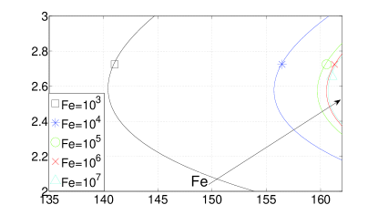
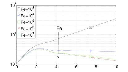
Figure 3: Effect of $Fe$. The parameters are $C=50$, $M=100$, $T=155$, $\alpha=2.5$, $\beta=0$ and $N=250$. The direction of the arrow indicates increasing $Fe$. (a) Neutral stability curves for various $Fe$. (b) $T_{c}$ as a function of $Fe$. (c) Transient energy growth versus time.

The role of $M$ in EHD is analogous to that of the Prandtl number in Rayleigh-Bénard convection. In figure 4(a), it is shown that the variation of $M$ exerts no influence on the linear stability criterion, $T_{c}=159.58$ at $C=100$, $Fe=10^{5}$, $\alpha=2.57$ and $\beta=0$; the same finding has been reported in Atten & Moreau (1972). For the transient dynamics, however, the same conclusion does not hold, as evidenced in figure 4(b). The plot describes a trend of increasing $G_{max}$ with smaller $M$. The slopes at the final time are slightly different for each $M$, indicating that the asymptotic growth rates differ slightly (while the linear stability criterion remains the same).

Figure 4: Effect of $M$. The parameters are $C=100$, $Fe=10^{5}$, $\alpha=2.57$, $\beta=0$ and $N=250$ without cross-flow. (a) The neutral stability curve. (b) Transient energy growth versus time for different $M$ and $T=155$. The direction of the arrow indicates increasing $M$.

Figure 5 depicts the influence on $C$, which measures the intensity of charge injection. Atten & Moreau (1972); Atten & Lacroix (1979) reported a dependence of the critical value $T_{c}$ on the parameter $C$. In figure 5(a), we see that, in the SCL regime, increasing $C$ will yield lower $T_{c}$. This result can be understood from a physical argument. Increasing the intensity of charge injection will lead to a higher concentration of charges between the electrodes. The linear instability mechanism, as discussed before, relies on the formation of an electric torque due to convective motions. With higher charge concentration, the electric torque is stronger. Therefore, a lower voltage difference is required, which amounts to stating that a lower $T$ will be sufficient to form an electric torque of comparable strength. But as we are in the SCL regime (with a value of $C=50$ considered very large), a rise of $C$ to $200$ only yields a minor decrease in $T_{c}$. In contrast, the transient dynamics of the perturbation energy $G$ appears not to be influenced by a change in $C$ for early times; for example, see the time interval $t\in[0,3]$ in figure 5b.

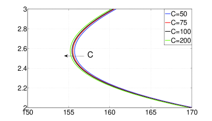
Figure 5: Effect of $C$. The parameters are $M=100$, $Fe=10^{4}$, $\beta=0$ and $N=250,$ without cross-flow. The direction of the arrow indicates increasing $C$. (a) Neutral stability curve for four different injection levels $C$ within the SCL regime. (b) Transient energy growth for different $C$ at $T=155,\alpha=2.57$.

4.2 EHD with cross-flow

When cross-flow is considered, the property of the linearized system changes due to the presence of a base shear in the flow. Especially, this shear will render the linearized operator ‘more non-normal’. We first note that, in the modal stability analysis, Squire’s theorem still holds for EHD-Poiseuille flow, that is, a two-dimensional instability will be encountered first. This can be easily verified by a perfect analogy with standard viscous theory (Schmid & Henningson, 2001). Moreover, there are two sets of scales in the EHD problem with cross-flow. To study the influence of the cross-flow on the electric and the charge fields, the values of $M$ and $T$ are kept in the vicinity of the values in the previous section: the scale of the electric field will be considered primarily, whereas, when we examine effects of the electric field exerted on the canonical Poiseuille flow, we take the value of the free parameter $Re$ around $5772$, i.e., the linear stability criterion for pressure-driven flow; the latter choice introduces a scale based on the hydrodynamics. In both cases, we will enforce the relation $Re=T/M^{2}$, which results in the Reynolds number $Re$ to be rather low in the former case (denoted as the low-$Re$ case) and relatively high in the latter case (referred to as the high-$Re$ case).

4.2.1 EHD: low $Re$

We have demonstrated that nonmodal effects in hydrostatic EHD are not significant. In the presence of cross-flow, given that the Reynolds number in this section is considered small, we expect the nonnormality to be rather moderate as well. For this reason, we will mainly focus on the modal stability characteristics for the low-$Re$ case.

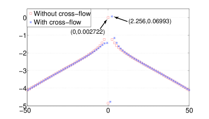
Figure 6: (a) Spectra for the case with and without cross-flow for $C=50$, $M=100$, $Fe=10^{5}$, $T=160$, $Re=T/M^{2}=0.016$ (for cross-flow), $\alpha=2.57$, $\beta=0$ and $N=250$. (b) Effect of $Fe$ on the neutral stability curve. The parameters are $C=50$, $M=100$, $\beta=0$ and $N=250,$ with cross-flow. The direction of the arrow indicates increasing $Fe$.

In figure 6(a), it is observed that the symmetry of the hydrostatic EHD spectrum is now broken due to the presence of cross-flow. The most unstable perturbation travels at a positive phase speed $u_{p}=\omega_{r}/\alpha=2.256/2.57=0.8778,$ induced by cross-flow convection (the centerline velocity of the cross-flow is $1,$ as we set $Re=T/M^{2}$ in equation (5)). In figure 6b, we show the neutral stability curve for $C=50$, $M=100$, $\beta=0$ and $N=250$, which can be directly compared to the results in figure 3. Note that since $Re=T/M^{2}$ is enforced, the Reynolds number $Re$ is not identical for each point, but generally small. We see that, with cross-flow, the critical $T_{c}$ decreases compared to the no-cross-flow case; this indicates that the flow is more unstable in the presence of a low-$Re$ cross-flow compared to the results in figure 3(a). To investigate the reason behind this destabilization, we again resort to an energy analysis in section 5.1.2. Previously, an energy analysis for EHD with cross-flow has been studied in Castellanos & Agrait (1992).

Figure 7: Effect of $M$. (a) Neutral stability curve with cross-flow for $C=100$, $Fe=10^{5}$, $\alpha=2.57$, $\beta=0$ and $N=250$. (b) Transient energy growth for different $M$ and $T=145$. The direction of the arrow indicates increasing $M$.

Even though varying $M$ has no effect on the linear stability when $\bar{U}=0,$ as has been discussed briefly in the previous section, in the presence of cross-flow, changing $M$ does influence the linear stability. This is displayed in figure 7(a), where we see that effects of $M$ are only discernable when $M$ is small. We will discuss this issue further in the energy analysis section 5.1.2. Considering non-normal linear stability, transient energy growth $G$ is still small, even though slightly higher than in the no-cross-flow case.

4.2.2 EHD: high $Re$

In this section, we consider the flow governed by the inertial scale, i.e., in the high-$Re$ regime. To discuss the results more properly, the Reynolds number $Re$ will be the free parameter, and the governing momentum equation is given by (6), see section 2.3. The modal stability is examined in figure 8. In subfigure (a), changes in the spectrum due to the additional electric field are visible. It appears that the core modes, wall modes and center modes do not change appreciably, except that the growth rate of the most unstable mode increases. In subfigure (b), we plot the neutral stability curve for varying $T$. The pure hydrodynamic linear stability limit $Re=5772.2$ is recovered by considering a minute value for $T$ such as $T=10^{-8}$ (we could have taken $T=0$, but to be compatible with equation (2.3) and the discussion based on that equation in other literature, we assign to $T$ a negligibly small value). With increasing $T$, the system becomes more unstable, as the critical linear stability criterion becomes smaller. The reason for this is obviously due to the effect of the electric field transferring energy into the velocity fluctuations, while at the same time modifying the canonical channel flow; see table 3 in the energy analysis section 5.1.3 at $C=100,Fe=10^{5},Re=5500,\alpha=1$ and $\beta=0$.

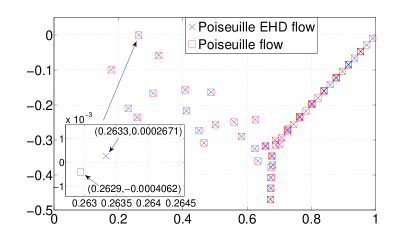
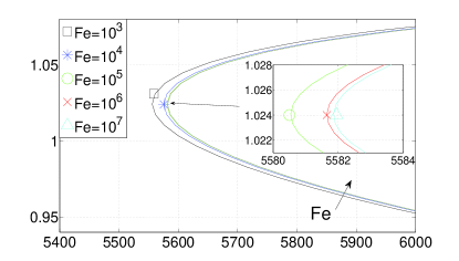
Figure 8: (a) Comparison of two spectra for $T=10^{-8}$ and $T=200$ at $C=100,Re=5600,Fe=10^{5},\alpha=1,\beta=0$. (b) Effect of $T$ on the neutral stability curve with cross-flow at $C=100$, $Fe=10^{5}$, $M=\sqrt{T/M^{2}}$, $\beta=0$. The direction of the arrow indicates increasing $T$. (c) Effect of $Fe$ on the neutral stability curve with cross-flow at $C=100,T=100,M=\sqrt{T/M^{2}},\beta=0$. The direction of the arrow indicates increasing $Fe$.

We also investigate the effect of charge diffusion $Fe$ on the flow stability. The results concerning the neutral stability curve are shown in figure 8(c) at $C=100,T=100,M=\sqrt{T/M^{2}},\beta=0$. For small charge diffusion (large $Fe$), the critical Reynolds number $Re$ is only slightly affected by changes in $Fe$. Only when $Fe=10^{3}$ does the critical Reynolds number $Re$ drop noticeably, though the destabilization effect is still small. It thus can be concluded that charge diffusion has only a small influence on the dynamics of EHD cross-flow at high $Re$. This is due to the inertial scale we are considering. As we have seen in the hydrostatic EHD flow, the effect of charge diffusion is significant, considering the electric scale, i.e., at relatively small (or zero) Reynolds numbers.

It is well known that in high-$Re$ Poiseuille flow the two-dimensional Orr mechanism is not the principal mechanism for perturbation energy growth over a finite time horizon. The flow is expected to become turbulent within a short time interval, even though the asymptotic growth rate of the linear system is negative. The non-normal nature of the linearized Navier-Stokes operator for channel flow — in physical terms, due to the base flow modulation by spanwise vorticity tilting into the wall-normal direction — suggests that transient disturbance growth during the early phase should be considered primarily.

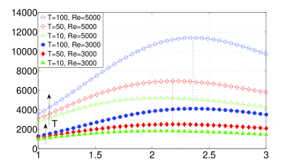
Figure 9: Effect of $T$. The direction of the arrow indicates increasing $T$. (a) Transient energy growth for $C=100$, $Re=5200$, $Fe=10^{5}$, $\alpha=0$, $\beta=2$. (b) Contours of transient growth $G$ in the $\alpha$-$\beta$-plane at $C=100,Re=5000,Fe=10^{5},T=100$. (c) Transient growth $G$ as a function of $\beta$ at $C=100$, $Fe=10^{5}$, $\alpha=0$.

In figure 9(a), we present the transient growth $G$ for different $T$. Mainly, the effect of increasing $T$ is to enhance transient growth. The optimal initial condition which achieves maximum transient growth is shown in figure 9(b). The optimal wavenumbers for the pure hydrodynamic case, independent of $Re$, are found to be $\alpha=0$ and $\beta=2.05,$ suggesting streamwise-independent vortices as the most amplified structures (Schmid & Henningson, 2001). For high-$Re$ EHD with cross-flow, the maximum transient growth is still found to favor streaks ($\alpha=0$), but with a different optimal spanwise wavenumber of $\beta=2.36$ at $C=100,Re=5000,Fe=10^{5},T=100$ (see figure 9(b)). Interestingly, for a different value of $T$, i.e., a different amount of potential drop across the electrodes, the optimal wavenumber would be different. For example, at $T=50$ the optimal $\beta=2.18,$ while at $T=10$ the optimal $\beta=2.08$, as shown in figure 9(c). It seems that, for smaller $T$, approaching the regime of pure hydrodynamics, the optimal $\beta$ is converging towards $\beta=2.05$. The independence of maximum transient growth on $Re$ for various $\beta$ still holds in the limit of high-$Re$ EHD flow, as indicated by the dashed lines connecting the peaks of the two curves for $Re=5000$ and $Re=3000$ in figure 9(c). In the nonlinear regime of EHD Poiseuille flow, the influence of the electric field on the streaks has been reported in Soldati & Banerjee (1998). These authors reported the spanwise spacing of the low-speed streaks are about $105\pm 15$ in wall units, which is different from the average spanwise spacing of the streaks in Poiseuille flow, that is $100$ in wall units, see Butler & Farrell (1993) for example. Thus, to some extent, our results that the spanwise spacing of the streaks changes in the linear EHD cross-flow agree qualitatively with these findings. These authors also found that the cross-flow is weakened by the electric field. This does not stand in conflict with the current results, because enhanced transient growth due to the electric field, as found here, only indicates that, in the linear phase, transition to turbulence is more rapid when compared to canonical channel flow; no conclusions can be drawn for the flow behavior in the nonlinear regime. To more fully understand how the electric field influences streaks and streamwise vortices in the nonlinear phase of transition, a more comprehensive study of the role played by EHD in the formation and dynamics of a self-sustaining cycle (Jiménez & Pinelli, 1999) is called for.

To further investigate the effect of $T$, we plot in figure 10 the optimal initial conditions which achieve $G_{max}$ in a given finite time for parameters $C=100$, $Re=5000$, $Fe=10^{5}$, $\alpha=0$ and different values of $T$ with its corresponding optimal $\beta$. In subfigure (a), the optimal initial conditions for $v$ for various $T$ are presented. The symmetry of the optimal $v$ with respect to the flow centerline $y=0,$ when the flow is close to the pure-hydrodynamics limit, is broken due to the action of the electric field in the wall-normal direction as $T$ increases. Since the electrode with higher potential is at $y=1$ in our case, the optimal initial conditions for $w$ and $v$ are tilted towards $y=1$ (see also subfigure (b), which additionally shows the optimal initial condition for $\varphi$). In subplot (c), the formation of streamwise vortices in the $y$-$z$-plane is shown; their centers are shifted upwards by the electric field. In subfigure (d), the optimal response of $\varphi$, taking the form of waves in the spanwise direction, is displayed. Recalling that the nonmodal transient growth is due to base-flow modulations arising from the tilting of spanwise into wall-normal vorticity, we can state that the variation of the optimal spanwise wavenumber for different $T$ is the direct result of the three-dimensional nature of the non-normal linearized operator under the influence of a constant electric field pointing in the wall-normal coordinate direction.

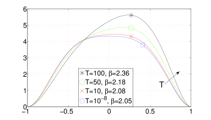
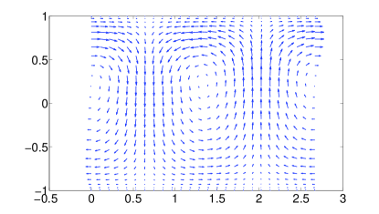
Figure 10: Effect of $T$. (a) The optimal initial condition for $v$ as a function of $T$ and $\beta$ at $C=100$, $Fe=10^{5}$, $Re=5000$, $\alpha=0$. (b) The optimal initial conditions of velocity and potential at $C=100$, $Re=5000$, $Fe=10^{5}$, $T=100$, $\alpha=0$, $\beta=2.36$. (c) Velocity vectors of the optimal initial condition in the cross-stream plane; same parameters as in (b). (d) Contour of the optimal response for $\varphi$; same parameters as in (b).

5 Results of energy analysis

5.1 Asymptotic energy analysis

The dynamics of the disturbance energy (of the velocity fluctuations) in the limit of an infinite time horizon is examined in this section. The governing equation for the energy evolution is obtained by multiplying the linearized equation (2.3b) by the complex conjugate velocity $v_{i}^{\dagger}$, i.e.,

$$v_{i}^{\dagger}\frac{\partial v_{i}}{\partial t}+v_{i}^{\dagger}v_{j}\frac{\partial\bar{U}_{i}}{\partial x_{j}}+v_{i}^{\dagger}\bar{U}_{j}\frac{\partial v_{i}}{\partial x_{j}}=-v_{i}^{\dagger}\frac{\partial p}{\partial v_{i}}+v_{i}^{\dagger}\frac{M^{2}}{T}\frac{\partial^{2}v_{i}}{\partial x_{j}^{2}}+v_{i}^{\dagger}M^{2}(\frac{\partial\bar{\phi}}{\partial x_{i}}\frac{\partial^{2}\varphi}{\partial x_{j}x_{j}}+\frac{\partial^{2}\bar{\phi}}{\partial x_{j}x_{j}}\frac{\partial\varphi}{\partial x_{i}}),$$ (19)

taking the complex conjugate of the obtained equation, and averaging the two equations, which leaves us with

$$\frac{\partial\mathcal{E}}{\partial t} = -\frac{1}{2}(v_{i}^{\dagger}v_{j}+v_{j}^{\dagger}v_{i})\frac{\partial\bar{U}_{i}}{\partial x_{j}}-\frac{M^{2}}{T}\frac{\partial v_{i}^{\dagger}}{\partial x_{j}}\frac{\partial v_{i}}{\partial x_{j}}-\frac{M^{2}}{2}\frac{\partial\bar{\phi}}{\partial x_{i}}(\frac{\partial\varphi^{\dagger}}{\partial x_{j}}\frac{\partial v_{i}}{\partial x_{j}}+\frac{\partial\varphi}{\partial x_{j}}\frac{\partial v_{i}^{\dagger}}{\partial x_{j}})$$ (20)

$$-\frac{M^{2}}{2}\frac{\partial^{2}\bar{\phi}}{\partial x_{i}\partial x_{j}}(v_{i}^{\dagger}\frac{\partial\varphi}{\partial x_{j}}+v_{i}\frac{\partial\varphi^{\dagger}}{\partial x_{j}})-\frac{M^{2}}{2}\frac{\partial^{3}\bar{\phi}}{\partial x_{i}\partial x_{i}\partial x_{j}}(\varphi v_{j}^{\dagger}+\varphi^{\dagger}v_{j})$$

$$+\frac{\partial}{\partial x_{j}}\left[-\frac{1}{2}v_{i}v_{i}^{\dagger}\bar{U}_{j}-\frac{1}{2}(v_{i}^{\dagger}p+v_{i}p^{\dagger})\delta_{ij}+\frac{M^{2}}{2T}(v_{i}^{\dagger}\frac{\partial v_{i}}{\partial x_{j}}+v_{i}\frac{\partial v_{i}^{\dagger}}{\partial x_{j}})\right.$$

$$+\left.\frac{M^{2}}{2}\frac{\partial\bar{\phi}}{\partial x_{i}}(\frac{\partial\varphi}{\partial x_{j}}v_{i}^{\dagger}+\frac{\partial\varphi^{\dagger}}{\partial x_{j}}v_{i})+\frac{M^{2}}{2}\frac{\partial^{2}\bar{\phi}}{\partial x_{i}x_{i}}(\varphi v_{j}^{\dagger}+\varphi^{\dagger}v_{j})\right],$$

where $\mathcal{E}=v_{i}^{\dagger}v_{i}/2$ is the perturbation energy density of the hydrodynamic part in the spectral space. The terms in the square brackets are the transport terms which, in case of periodic as well as no-slip and no-penetration boundary conditions , exert no influence on the energy balance. Therefore, after integrating the above equation over the control volume $\Omega$, we obtain

$$\int_{\Omega}\frac{\partial\mathcal{E}}{\partial t}\ dV= - \underbrace{\int_{\Omega}\frac{1}{2}(v_{i}^{\dagger}v_{j}+v_{j}^{\dagger}v_{i})\frac{\partial\bar{U}_{i}}{\partial x_{j}}\ dV}_{{\mathsf{Pr}}}-\underbrace{\int_{\Omega}\frac{M^{2}}{T}\frac{\partial v_{i}^{\dagger}}{\partial x_{j}}\frac{\partial v_{i}}{\partial x_{j}}\ dV}_{{\mathsf{VD}}}$$ (21)

$$- \underbrace{\int_{\Omega}\frac{M^{2}}{2}\frac{\partial\bar{\phi}}{\partial x_{i}}\left(\frac{\partial\varphi^{\dagger}}{\partial x_{j}}\frac{\partial v_{i}}{\partial x_{j}}+\frac{\partial\varphi}{\partial x_{j}}\frac{\partial v_{i}^{\dagger}}{\partial x_{j}}\right)\ dV}_{{\mathsf{VE1}}}$$

$$- \underbrace{\int_{\Omega}\frac{M^{2}}{2}\frac{\partial^{2}\bar{\phi}}{\partial x_{i}\partial x_{j}}\left(v_{i}^{\dagger}\frac{\partial\varphi}{\partial x_{j}}+v_{i}\frac{\partial\varphi^{\dagger}}{\partial x_{j}}\right)\ dV}_{{\mathsf{VE2}}}$$

$$- \underbrace{\int_{\Omega}\frac{M^{2}}{2}\frac{\partial^{3}\bar{\phi}}{\partial x_{i}\partial x_{i}\partial x_{j}}(\varphi v_{j}^{\dagger}+\varphi^{\dagger}v_{j})\ dV}_{{\mathsf{VE3}}}.$$

Since the boundary conditions are periodic in the wall-parallel coordinate directions, it is legitimate to consider the control “volume” $\Omega$ only in the $y$-direction, that is, $\Omega=[-1,1]$ and $dV=dy.$ The first term on the right-hand side of equation (21) represents energy production from the mean shear (${\mathsf{Pr}}$), which is zero in the hydrostatic case; the second term describes viscous dissipation (${\mathsf{VD}}$); the third to fifth terms are the energy transfer terms between the velocity fluctuation field and the electric field (${\mathsf{VE1}}$, ${\mathsf{VE2}}$, ${\mathsf{VE3}},$ respectively). The Einstein summation convention does not apply for the subscripts of ${\mathsf{VE1}}_{ij}$, for example; the term ${\mathsf{VE1}}_{21}$, for instance, represents $\displaystyle{\int_{\Omega}}\displaystyle{\frac{M^{2}}{2}}\displaystyle{\frac{\partial\bar{\phi}}{\partial y}}\left(\frac{\partial\varphi^{\dagger}}{\partial x}\frac{\partial v}{\partial x}+\frac{\partial\varphi}{\partial x}\frac{\partial v^{\dagger}}{\partial x}\right)\ dV$.

As has been discussed and verified for polymeric flows in Zhang et al. (2013), the time variation of the normalized perturbation energy density should be equal to the twice the asymptotic growth rate of linear disturbances, i.e.,

$$R_{e}=\frac{\displaystyle{\int_{\Omega}}\displaystyle{\frac{\partial\mathcal{E}}{\partial t}}\ dV}{\displaystyle{\int_{\Omega}}\mathcal{E}dV}=2\omega_{i},$$ (22)

where $\omega_{i}$ denotes the growth rate of the least stable mode. We will validate this relation in the following sections and use it as an a posteriori check for our results.

5.1.1 EHD without cross-flow

We apply the energy analysis for hydrostatic EHD flow with different values of charge diffusion coefficients $Fe$ to probe how the electric field interacts with the velocity fluctuations. Quantitative results are listed in table 1, with the notation ${\mathsf{VD}}={\mathsf{VD}}_{11}+{\mathsf{VD}}_{12}+{\mathsf{VD}}_{21}+{\mathsf{VD}}_{22}$ and, likewise, ${\mathsf{VE}}={\mathsf{VE1}}_{21}+{\mathsf{VE1}}_{22}+{\mathsf{VE2}}+{\mathsf{VE3}}$. No spanwise dependence as $\beta=0$. Immediately, one can make several direct observations. First, viscous dissipation is always negative for the hydrodynamics. Second, since the EHD flow is hydrostatic, there is no production from the mean shear, ${\mathsf{Pr}}=0$. The only terms that can lead to growths in the hydrodynamic disturbance energy density $\mathcal{E}$ are linked to the energy transfer from the electric field, ${\mathsf{VE}}$. The most efficient mechanism seems to be related to the term ${\mathsf{VE1}}_{21}$, which represents the interaction between the streamwise perturbed electric field and the wall-normal velocity shear under the constant effect of the wall-normal base electric field. The term ${\mathsf{VE3}}$ is even negative, indicating that the electric field can absorb energy from the perturbed hydrodynamic field by an out-of-phase configuration between $\varphi$ and $v$ (in the energy-budget equation for the perturbed electric field, one would find the exact same term with opposite sign). Regarding the effect of charge diffusion, with increasing $1/Fe$ (increasing charge diffusion) from the right column to the left in the table, the total energy transfer ${\mathsf{VE}}$ diminishes, but, at the same time, the hydrodynamic diffusion is also dissipating less energy into heat. Furthermore, even though ${\mathsf{VE}}$ (and thus ${\mathsf{VE1}}_{22}$, ${\mathsf{VE2}}$ and ${\mathsf{VE3}}$) decreases with rising charge diffusion, the primary mechanism of energy transfer ${\mathsf{VE1}}_{21}$ transfers more energy from the electric field to the hydrodynamic fluctuations, together with a less dissipation, leading to an unstable flow for the chosen parameters. Therefore, it seems that the effect of charge diffusion is to catalytically enhance the efficiency of the most productive energy transfer mechanism between the perturbed electric field and the hydrodynamics, expressed by the term ${\mathsf{VE1}}_{21}$, and result in a lower dissipation. As a consequence, increasing charge diffusion leads to a more unstable flow.

terms	$Fe=10^{4}$	$Fe=10^{5}$	$Fe=10^{6}$	$Fe=10^{7}$
${\mathsf{VD}}_{11}$	-254.9836	-255.3751	-255.4628	-255.4781
${\mathsf{VD}}_{12}$	-481.9379	-486.1119	-487.0231	-487.1773
${\mathsf{VD}}_{21}$	-570.6289	-570.2374	-570.1497	-570.1344
${\mathsf{VD}}_{22}$	-254.9836	-255.3751	-255.4628	-255.4781
${\mathsf{VE1}}_{21}$	1154.1206	1152.8793	1152.6403	1152.5936
${\mathsf{VE1}}_{22}$	428.695	431.8134	432.4984	432.6197
${\mathsf{VE2}}$	30.0141	30.7628	30.9299	30.9614
${\mathsf{VE3}}$	-50.2196	-48.3506	-47.9797	-47.9186
${\mathsf{VD}}$	-1562.5341	-1567.0994	-1568.0984	-1568.2679
${\mathsf{VE}}$	1562.6102	1567.1049	1568.089	1568.2561
${\mathsf{Pr}}$	0	0	0	0
$R_{e}$	0.0761	0.0054	-0.0094	-0.0119
$2\omega_{i}$	0.0761	0.0054	-0.0094	-0.0119

Table 1: Energy budget for modal instability of hydrostatic EHD flow for different values of the charge diffusion. The results are normalized as in equation (22). The parameters are $C=50$, $M=100$, $T=160$, $\alpha=2.57$, $\beta=0$ for hydrostatic flow.

It is instructive to assess the effect of $M$ on the linear stability (see section 4.1) with the help of the energy-budget equation (21). For a vanishing time derivative of the energy density, the factor $M^{2}$ on the right-hand side can be eliminated for the hydrostatic case $\bar{U}=0$. In the case of cross-flow, however, with the same reasoning $M$ will have an influence on the linear stability criterion.

5.1.2 EHD with low-$Re$ cross-flow

Table 2 shows the results for $C=50$, $M=100$, $T=160$, $Re=T/M^{2}=0.016$, $\alpha=2.57$, $\beta=0$ with cross-flow for different $Fe$. Compared to the case without cross-flow, the results are quite similar. However, it is interesting to note that the fluctuation energy production from the mean shear ${\mathsf{Pr}}$, even though rather small, is negative, indicating that the perturbed flow field transfers energy to the base flow. Recalling the results in figure 7 of section 4.2.1, a change of $M$ does not have a strong effect on the rate of change of the disturbance energy density ${\mathsf{E}}$ since ${\mathsf{Pr}}$ is very small.

In the case of EHD flow with a weak cross-flow ($Re=0.016$), the main mechanism for transferring energy into the hydrodynamic subsystem is still based on the potential difference across the two electrodes — the same as for the no cross-flow case. This can be confirmed by inspecting table 2: ${\mathsf{VE1}}_{21}$ is the dominant energy transfer term.

terms	$Fe=10^{4}$	$Fe=10^{5}$	$Fe=10^{6}$	$Fe=10^{7}$
${\mathsf{VD}}_{11}$	-254.1325	-254.1337	-254.1318	-254.1309
${\mathsf{VD}}_{12}$	-475.0779	-476.292	-476.5068	-476.5348
${\mathsf{VD}}_{21}$	-571.48	-571.4788	-571.4807	-571.4816
${\mathsf{VD}}_{22}$	-254.1325	-254.1337	-254.1318	-254.1309
${\mathsf{VE1}}_{21}$	1158.7772	1157.62	1157.3579	1157.3025
${\mathsf{VE1}}_{22}$	422.786	423.6012	423.7687	423.7989
${\mathsf{VE2}}$	26.3245	26.363	26.3747	26.3794
${\mathsf{VE3}}$	-52.8799	-51.3981	-51.1094	-51.0629
${\mathsf{VD}}$	-1554.8229	-1556.0382	-1556.2511	-1556.2782
${\mathsf{VE}}$	1555.0078	1556.1861	1556.3919	1556.4179
${\mathsf{Pr}}$	-0.0079038	-0.0080187	-0.0080507	-0.0080566
$R_{e}$	0.1769	0.1399	0.1327	0.1316
$2\omega_{i}$	0.1769	0.1399	0.1327	0.1316

Table 2: Energy budget for modal instability of EHD flow with low-$Re$ cross-flow for different values of the charge diffusion $Fe$. The results are normalized as in equation (22). The parameters are $C=50$, $M=100$, $T=160$, $Re=T/M^{2}=0.016$, $\alpha=2.57$, $\beta=0$ with cross-flow.

5.1.3 EHD with high-$Re$ cross-flow

terms  $(\times 10^{-4})$	$T=10^{-8}$	$T=10$	$T=100$	$T=200$
${\mathsf{VD}}_{11}$	-2.643	-2.643	-2.6429	-2.6429
${\mathsf{VD}}_{12}$	-138.22	-138.24	-138.42	-138.61
${\mathsf{VD}}_{21}$	-0.99338	-0.99339	-0.99343	-0.99347
${\mathsf{VD}}_{22}$	-2.643	-2.643	-2.6429	-2.6429
${\mathsf{VE1}}_{21}$	3.1782 $\!\cdot 10^{-10}$	0.31785	3.1814	6.3689
${\mathsf{VE1}}_{22}$	7.3458 $\!\cdot 10^{-10}$	0.73467	7.355	14.729
${\mathsf{VE2}}$	7.0501 $\!\cdot 10^{-11}$	0.070507	0.70555	1.4122
${\mathsf{VE3}}$	-1.2043 $\!\cdot 10^{-10}$	-0.12044	-1.2055	-2.4133
${\mathsf{VD}}$	-144.5	-144.52	-144.7	-144.89
${\mathsf{VE}}$	10.025 $\!\cdot 10^{-10}$	1.0026	10.036	20.096
${\mathsf{Pr}}$	132.35	132.06	129.41	126.44
$R_{e}$	-12.153	-11.463	-5.2526	1.6542
$2\omega_{i}$	-12.153	-11.463	-5.2526	1.6542

Table 3: Energy budget for modal instability of EHD flow with a high-$Re$ cross-flow for different values of the stability parameter $T$. The results are normalized as in equation (22). The parameters are $C=100$, $Fe=10^{5}$, $Re=5500$, $\alpha=1$ and $\beta=0$ with cross-flow.

The energy analysis for the EHD Poiseille flow at $C=100$, $Fe=10^{5}$, $Re=5500$, $\alpha=1$ and $\beta=0$ is summarized in table 3. Note that the production ${\mathsf{Pr}}$ is dimishing with increasing $T$. On the other hand, ${\mathsf{VE}}$ increases with larger values of $T$, compensating and exceeding the decrease of ${\mathsf{Pr}}$ at higher $T$. This is consistent with the results in figure 8: higher values of $T$ yield a more unstable flow. However, the principal mechanism underlying the flow instability is still linked to the production ${\mathsf{Pr}}$. The electric field only assumes a secondary role in destabilizing the flow, at least for the parameters considered in this case. Unlike the hydrostatic case where ${\mathsf{VE1}}_{21}$ is responsible for the dominant energy transfer, in the presence of cross-flow ${\mathsf{VE1}}_{22}$ becomes the most efficient agent transferring fluctuation energy ${\mathcal{E}}$ between the electric field and the perturbed velocity field.

5.2 Transient energy analysis

To investigate the cause for the increase of nonmodal growth with $T$, recall figure 9, we formulate and perform an energy analysis for the initial-value problem of equation (10). We consider the energy density evolution over a finite time horizon following Butler & Farrell (1992)

$$\frac{1}{|\Omega|}\int_{\Omega}\frac{\partial\mathcal{E}}{\partial t}\ dV = \frac{1}{|\Omega|}\int_{-1}^{1}\int_{0}^{a}\int_{0}^{b}\frac{\partial}{\partial t}\left(\frac{u^{2}+v^{2}+w^{2}}{2}\right)\ dV$$

$$= \frac{1}{|\Omega|}\int_{-1}^{1}\int_{0}^{a}\int_{0}^{b}\underbrace{\left[-uv\frac{dU}{dy}\right.}_{{\mathsf{Pr}}}-\underbrace{\frac{1}{Re}\frac{\partial u_{i}}{\partial x_{j}}\frac{\partial u_{i}}{\partial x_{j}}}_{{\mathsf{VD}}}$$

$$\phantom{123456}-\underbrace{\frac{T}{Re}\frac{\partial\bar{\phi}}{\partial y}\frac{\partial\varphi}{\partial x_{j}}\frac{\partial v}{\partial x_{j}}}_{{\mathsf{VE1}}}-\underbrace{\frac{T}{Re}\frac{\partial^{2}\bar{\phi}}{\partial y^{2}}v\frac{\partial\varphi}{\partial y}}_{{\mathsf{VE2}}}-\underbrace{\left.\frac{T}{Re}\frac{\partial^{3}\bar{\phi}}{\partial y^{3}}\varphi v\right]}_{{\mathsf{VE3}}}\ dz\ dx\ dy$$

where $|\Omega|=2ab$, $a=2\pi/\alpha$ and $b=2\pi/\beta$. In the above equation, we label, as before, the first term on the right-hand side as ${\mathsf{Pr}}$ (production from the mean shear), the second term as ${\mathsf{VD}}$ (viscous dissipation), the third to fifth terms collectively as ${\mathsf{VE}}$ (energy density transfer between the perturbed velocity field and the perturbed electric field) and the sum of all five terms as ${\mathsf{Total}}$. In this temporal evolution problem, the initial condition is the optimal one, following the procedure in section 4.2.2.

Results of our energy analysis are presented in figure 11. In subfigure (a) and its inset, the pure hydrodynamic result is shown, where the production ${\mathsf{Pr}}$ counteracts the viscous dissipation ${\mathsf{VD}}$. In subplot (b) for EHD cross-flow, we observe that the term ${\mathsf{VE}}$ is insignificant, even though at $T=100$; this is in contrast to both the linear modal stability criterion (see figure 8) and the overall nonmodal transient growth (see figures 9 and 10) where its effect is not negligible. Furthermore, production ${\mathsf{Pr}}$ increases by a factor of $2\sim 3$ compared to the pure hydrodynamic flow. These results seem to indicate that, concerning the nonmodal analysis, the effect of the additional electric field on the canonical channel flow is incidental, i.e., the perturbation velocity energy is only indirectly influenced by the electric field; in fact, the electric field does not induce a substantial energy transfer directly into velocity fluctuations at all and its effect is to enhance the lift-up mechanism, therefore the production.

Examining more closely the inset in figure 11(b), we see that the term ${\mathsf{VE}}$ surpasses ${\mathsf{Pr}}$ only in the very beginning of the time horizon. This is due to the high-$Re$ regime we are investigating. As discussed earlier, $Re={T}/{M^{2}}$ represents the ratio of the momentum relaxation time $L^{*2}/\nu^{*}$ to the charge relaxation time $L^{*2}/(K^{*}\Delta\phi_{0}^{*})$. With the maximum ${\mathsf{Total}}$ energy achieved at $t_{max}\approx 144$ in figure 11(b), we can estimate the time horizon in the inset by observing that $144/5000=0.029$, a value close to the time scale depicted in the inset of (b). Moreover, the minimal energy growth due to the electric force validates our previous observation that the purely EHD-induced non-normality is rather small (see appendix B for a direct proof of this statement via an input-output formulation). In the case of other complex flows at high Reynolds numbers, a similar conclusion can be draw, for instance, in viscoelastic flows (Zhang et al., 2013; Brandt, 2014), polymer stretching cannot induce disturbance growth when the fluid inertia is prevalent.

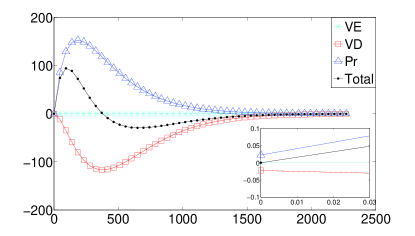
Figure 11: Energy analysis over a finite time horizon at $C=100$, $Re=5000$, $Fe=10^{5}$, $\alpha=0.$ (a) $T=10^{-8}$, $\beta=2.05;$ (b) $T=100$, $\beta=2.36$.

6 Discussion and conclusions

In this article, we have presented a comprehensive linear stability analysis of charge-injection-induced electrohydrodynamic flows between two plate electrodes, covering the hydrostatic as well as the cross-flow case, employing modal as well as nonmodal tools. We intend to examine whether the linear framework is sufficient for describing the transition to turbulence of EHD flow in the early phase of perturbation evolution. It is hoped that the results presented above and summarized below would help to understand better the EHD flow instability and its transition mechanism and shed light on its flow physics as well as flow control design.

6.1 EHD without cross-flow

In the hydrostatic case, the often-omitted charge diffusion is taken into account and found to have a non-negligible effect, particularly on the critical linear stability parameter $T_{c}$ with SCL injection — a finding running contrary to a common assumption in previous studies. In those studies, a linear stability analysis predicts a critical value of $T_{c}\approx 161$ in the strong injection limit. This result is reproduced in our computations for a negligible value of $1/Fe,$ but even for a moderate amount of charge diffusion the flow quickly becomes more unstable. Hence, we suggest that charge diffusion be accounted for in linear stability analyses and numerical simulations whenever the real physics indicates charge diffusion that can not be neglected, as it improves not only the model of the flow physics but also the robustness of the numerics as well. In fact, the common use of total variation diminishing (TVD) schemes (Harten, 1983) in direct numerical simulations of EHD flow, which introduces artificial numerical diffusion, seems unnecessary when true physical charge diffusion could be included.

The longstanding discrepancy of the critical stability parameter $T_{c}$ between the experimental and theoretical value, however, could not be resolved by our analysis: even though $T_{c}$ in the SCL limit drops to $140$ at $Fe=10^{3}$ (a physical value according to Pérez & Castellanos (1989)), a substantial gap remains to the experimentally measured parameter of $T_{c}\approx 110.$ Motivated by the researches in subcritical channel flow, we examine other mechanisms for early transition to turbulence, specifically, transient growth due to the non-normality of the linearized EHD operator. Nonmodal stability theory has been successfully applied to the variety of wall-bounded shear flows in an attempt to explaining aspects of the transition process. In the case of hydrostatic EHD flow, our calculations seem to indicate that transient energy growth, as defined in equation (13), is not significant, reaching gains of $\sim 10$ at most: the flow instability is rather dictated by the asymptotic growth rate of the least stable mode. These results seem to indicate that below the critical $T_{c}$ the significant energy growth observed in the real EHD flow is not of a linear nature, otherwise the linear framework would succeed to detect it. It might be hypothesized that the major energy growth mechanism in subcritical hydrostatic EHD follows a nonlinear route; nevertheless, it is only after performing a full nonlinear simulation of subcritical EHD flow that can one conclude whether its energy growth mechanism is truly nonlinear or not. Besides, these results also seem to shed some light on the flow control of hydrostatic EHD. It is now well-established that in canonical channel flow, where the perturbation energy is found to grow linearly in the early phase, a linear flow control strategy is sufficient to abate the perturbation development (Kim, 2003; Kim & Bewley, 2007). Due to the limited early perturbation energy growth in hydrostatic EHD, we thus suggest that different flow control methods be examined and applied in addressing the flow control of such flow. There might exist another possibility for the limited transient growth. As discussed by Atten (1974), the correct prediction of the linear stability criterion might require a closer comparison between the experimental conditions and the mathematical model. In this light, one may suggest a re-examination of the charge creation and transport processes, as the current charge creation model does not seem to accommodate any efficient energy transfer from the electric to the flow field, during the linear phase.

6.2 EHD with cross-flow

The flow instability and the transition to turbulence in canonical or complex channel (for example, EHD, MHD or polymeric) flows are currently not well understood. The study on the complex channel flow, serving as a supplement to the investigation of the canonical flows, focuses on the flow modification under the influence of external fields, for example, electric field, magnetic field or polymer stress field. The study of such flows will not only improve our understanding of these particular flow configurations, but also, more importantly, help us to better understand, during the linear, transition and turbulent phases, the dynamics of the important flow structures, for instance, the streak formation and attenuation, by probing the interaction between the fluids (or flow structures) and the external fields. For example, in the point of view of flow control, the research on polymer turbulence drag reduction reveals the mechanism how the auto-generation cycles of turbulence is modified in the presence of polymer molecules (Dubief et al., 2004). This has led to an even broader picture of the dynamics of turbulence. Similarly, in the case of EHD, our goal is to understand how the flow changes in response to the electric effects and provide a physical interpretation. Below we present the results of EHD cross-flow. We differentiated low-$Re$ and high-$Re$ cases. For low-$Re$ flow, the effects of $M$ and $Fe$ are similar to those of the hydrostatic flow, with the linear stability criterion being smaller for low-$Re$ cross-flow when compared to hydrostatic flow.

The high-$Re$ case is more interesting. In both modal and nonmodal stability analyses, the canonical channel flow becomes more unstable, once an electric field is applied between the two electrodes. From an input-output and an energy analysis we found, however, that the energy growth directly related to the electric field is not significant and that the effect of the electric field on the flow instability is indirect. In general, in high-$Re$ channel flow, the maximum transient growth is achieved by vortices aligning along the streamwise coordinate direction and generating streamwise streaks via an efficient energy growth mechanism known as lift-up. These optimal streamwise vortices are symmetric with respect to the channel centerline for standard Poiseille flow. In contrast to other complex flows, in EHD flows the electric field, which always points in the wall-normal direction, actively participates in the formation of the streamwise rolls by accelerating the downward-moving fluid (note that, in our setting, the injector is at $y=1$). Consequently, this yields stronger transient growth via the lift-up mechanism, when compared to the common channel flow. In other words, the electric field provides wall-normal momentum. As has been discussed in Landahl (1980) and recently reviewed by Brandt (2014), the presence of wall-normal momentum will cause any three-dimensional, asymptotically stable or unstable shear flow to exhibit energy growth during a transient phase. In the present study, the role of the electric field is to provide the shear flow with such a source of wall-normal momentum and to strengthen the lift-up mechanism for EHD flow with high-$Re$ cross-flow. Besides, we also find that the optimal wavenumbers for maximum transient growth increase under a stronger electric effect. Since the electric field will help to establish streamwise vortices, it may constitute a good actuator for drag reduction techniques, using the two-dimensional rolls together with a flow control strategy as described in Schoppa & Hussain (1998); Soldati & Banerjee (1998).

Appendix A Code validation

We first perform a resolution check to examine the convergence of the results. The parameters in this case are $C=50$, $Fe=2000$, $Re=6000$, $T=100$, $M=\sqrt{T/Re}=0.129$, $\alpha=1$ and $\beta=0$. The eigenspectra for four different grid resolutions $N$ are shown in figure 12(a). The most unstable mode in these cases are listed in table 4. Satisfactory convergence, with increasing $N$, is observed.

Secondly, the EHD eigenvector, from using (18), is examined against a verified, pure hydrodynamic stability code employing the same spectral collocation method and solving the Orr-Sommerfeld-Squire system, see Schmid & Henningson (2001), as shown in figure 12 (b). The parameters for the EHD code are $C=50$, $M=10^{-11}$, $Fe=2000$, $Re=6000$, $T=M^{2}\cdot Re$, $\alpha=1$, $\beta=0$ and $N=250$ . The parameters for the hydrodynamic stability code are $Re=6000$, $\alpha=1$, $\beta=0$ and $N=250$. We see that the iteratively solved EHD eigenvector is the same as the pure hydrodynamic one, which is solved directly by the Matlab routine eig. For the computation of the transient amplification $G$ in equation (17), it is legitimate to include only the first several, most unstable modes (Schmid & Henningson, 2001), i.e., eigenmodes corresponding to eigenvalues with imaginary part smaller than a certain $\omega_{i}^{c}$ are discarded, see table 5 for a validation of this approach. The reason for a minor increase of $G,$ as more modes are included, is due to the newly incorporated eigenvectors, not because of an insufficiently refined grid.

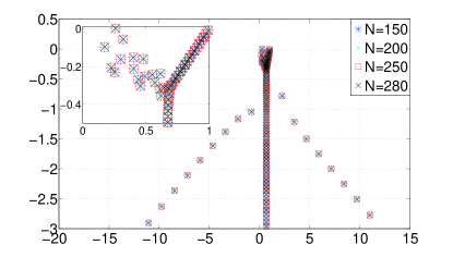
Figure 12: Code validation. (a) Resolution check for EHD flow with cross-flow at $C=50$, $Fe=2000$, $Re=6000$, $T=100$, $M=\sqrt{T/Re}=0.1291$, $\alpha=1$ and $\beta=0$. (b) Eigenvector component $v$ for the most unstable mode (normalized to have the same peak value for the two codes). The parameters are $C=50$, $M=10^{-11}$, $Fe=2000$, $Re=6000$, $T=M^{2}\cdot Re$, $\alpha=1$, $\beta=0$ and $N=250$ for the EHD code, and $Re=6000$, $\alpha=1$, $\beta=0$ and $N=250$ for the hydrodynamic stability code.

$N$	most unstable mode
$150$	$0.260023637950300+0.000652797815269i$
$200$	$0.260023637089882+0.000652796819289i$
$250$	$0.260023637069851+0.000652796791624i$
$280$	$0.260023637052960+0.000652796810920i$

Table 4: Code validation. Resolution check for the most unstable eigenvalue of EHD flow with cross-flow; with same parameters as in figure 12.

$\qquad\qquad\omega_{i}^{c}$	$G$			$\qquad\qquad\omega_{i}^{c}$	$G$
$-3.5$	$3.312404$			$-0.5$	$1.138543e+04$
$-5.5$	$3.434333$			$-3.5$	$1.174459e+04$
$-7.5$	$3.434351$			$-10.5$	$1.175565e+04$

Table 5: $G$ versus different cut-off growth rates $\omega_{i}^{c}$. The first two columns represent hydrostatic EHD flow at $C=50$, $Fe=10^{5}$, $M=100$, $T=155$, $\alpha=2.5$, $\beta=0$, $N=250$. The last two columns represent EHD flow with cross-flow at $C=100$, $Fe=10^{5}$, $Re=5000$, $T=100$, $\alpha=0$, $\beta=2.36$, $N=250$. Refer to the text for the definition of $\omega_{i}^{c}$.

With the eigenvalue problem reliably solved as shown above, we present validation for the specific flows considered here. In the case of hydrostatic flow, our results for $Fe=10^{7}$, approximating the case of zero charge diffusion, $T_{c}=160.67$ and $\alpha=2.57$ at $C=50$ (see figure 3(a) in section 4.1), are very close to the linear stability criterion reported in Atten & Moreau (1972), $T_{c}=160.75$ and $\alpha=2.569$ in the case of $C\rightarrow\infty$, where a coupled flow and electric system with neglected charge diffusion has been considered. This additionally implies that a value of $C$ higher than $50$ can well approximate the space-charge-limit.

In the presence of cross-flow, since there exist no quantitative results for eigenvalues and eigenvectors of the EHD problem in the literature, we partially verify our results by examining the pure hydrodynamic limit of the EHD-linearized problem, i.e., with electric effects being very small. This comparison is made with the stability code. The parameters are identical to the ones chosen above for the comparison of the eigenvectors. The Poiseuille base flow is $\bar{U}=1-y^{2}$ in both codes. It is obvious that, with these selected parameters, the governing equation (2.3.2c) for $\varphi$ is void of the coupling with $v,$ since $\bm{L}_{v\varphi}$ in equation (2.3.2a) is negligible. Therefore, the hydrodynamics equations for $v$ and $\eta$ in (2.3.2a) and (2.3.2b) must reproduce the results of the stability code. This match is shown in figure 13. In subfigure (a), the spectra of two codes are seen to collapse, even in the intersection region of the three eigenbranches, which is known to be sensitive due to the high non-normality of the linearized system (Schmid & Henningson, 2001). Additionally, the blue eigenmodes in (a) not matched by the red hydrodynamic modes are the supplementary eigenvalues linked to the presence of an electric field. The most unstable eigenvalue is shown in table 6. In subfigure (b), transient growth using an eigenvector expansion with $n=71$ eigenmodes is shown. A quantitative comparison of the maximum transient growth $G_{max}$ and its corresponding time $t_{max}$ is presented in in table 6. Agreement up to the fourth digit is achieved. The computations of $t_{max}$ and $G_{max}$ involve $n=71$ eigenfunctions, each one solved with the iterative method. Even though each individual mode may be prone to small inaccuracies, figure 13(b) illustrates that transient growth (a multi-modal phenomenon) can be reliably and robustly computed using the eigenvector expansion outlined above.

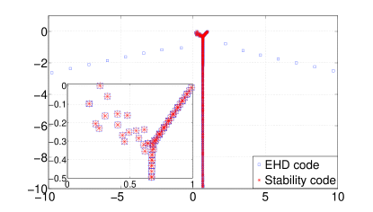
Figure 13: Comparison between EHD-Poiseuille flow and canonical Poiseuille flow. The parameters are $C=50$, $M=10^{-11}$, $Fe=2000$, $Re=6000$, $T=M^{2}\cdot Re$, $\alpha=1$, $\beta=0$ and $N=250$ for the EHD code, and $Re=6000$, $\alpha=1$, $\beta=0$ and $N=250$ for the purely hydrodynamic stability code. (a) The eigenvalue spectrum. (b) Transient amplification of initial energy.

	EHD code	hydrodynamic stability code
$\omega_{max,r}$	$0.259815871017297$	$0.259815871062631$
$\omega_{max,i}$	$0.000323088678313$	$0.000323088655527$
$t_{max}$	$18.86745$	$18.87514$
$G_{max}$	$38.92401$	$38.93307$

Table 6: Code validation. The parameters are the same as in figure 13.

Appendix B Input-output formulation

An input-output formulation can reveal additional information on prevalent instability mechanisms by considering different types of forcings (input) and responses (output) (Jovanović & Bamieh, 2005). To demonstrate that the transient growth due to perturbative $\varphi$ is small, we compare the full responses to perturbations consisting of (i) all variables $v,\eta$ and $\varphi$, (ii) both $v$ and $\eta$, and (iii) only $\varphi$. We thus define for these three cases different input filters $\bm{B}$, where $\bm{B}_{in1}=\bm{I}_{3N\times 3N}$ for the first case, while for the second and third cases we have

$$B_{in2}=\begin{pmatrix}\bm{I}_{N\times N}&\bm{0}\\ \bm{0}&\bm{I}_{N\times N}\\ \bm{0}&\bm{0}\end{pmatrix},\qquad\qquad B_{in3}=\begin{pmatrix}\bm{0}\\ \bm{0}\\ \bm{I}_{N\times N}\end{pmatrix}.$$ (24)

The output filter $\bm{C}_{out}$ is $\bm{I}_{3N\times 3N}$ for all three cases: we examine the flow response in all velocities and the electric field. Consequently, the energy weight matrices should be redefined with $\bm{\mathcal{M}}_{out}=\bm{C}_{out}\bm{\mathcal{M}}\bm{C}_{out}^{T}$ and $\bm{\mathcal{M}}_{in}=\bm{B}_{in}^{T}\bm{\mathcal{M}}\bm{B}_{in}$. After applying a Cholesky decomposition to these energy weight matrices, we obtain $\bm{F}_{out}$ and $\bm{F}_{in}$ for a formulation based on the $L_{2}$-norm. Finally, the maximum transient growth $G$ over a finite time interval is given by

$$G(t) = \underset{\bm{\gamma}_{0}}{\max}\frac{||\bm{\gamma}_{out}(t)||_{E_{out}}}{||\bm{\gamma}_{in}(0)||_{E_{in}}}=\underset{\bm{\gamma}_{0}}{\max}\frac{||\bm{\mathcal{T}}\bm{\gamma}_{in}(0)||_{E_{out}}}{||\bm{\gamma}_{in}(0)||_{E_{in}}}=\underset{\bm{\gamma}_{0}}{\max}\frac{||\bm{F}_{out}\bm{\mathcal{T}}\bm{\gamma}_{in}(0)||_{2}}{||\bm{F}_{in}\bm{\gamma}_{in}(0)||_{2}}$$ (25)

$$= \underset{\bm{\gamma}_{0}}{max}\frac{||\bm{F}_{out}\bm{\mathcal{T}}\bm{F}_{in}^{-1}\bm{F}_{in}\bm{\gamma}_{in}(0)||_{2}}{||\bm{F}_{in}\bm{\gamma}_{in}(0)||_{2}}=||\bm{F}_{out}\bm{\mathcal{T}}\bm{F}_{in}^{-1}||_{2}$$

$$= ||\bm{F}_{out}\bm{C}_{out}e^{t\bm{\mathcal{L}}}\bm{B}_{in}\bm{F}_{in}^{-1}||_{2}.$$

input		$B_{in1}\{v,\eta,\varphi\}$		$B_{in2}\{v,\eta\}$		$B_{in3}\{\varphi\}$
$t_{max}$		583.4087		587.7147		552.0443
$G_{max}$		11765.40		11350.38		428.8926

Table 7: Result from an input-output analysis at $C=100$, $Fe=10^{5}$, $Re=5000$, $T=100$, $\alpha=0$ and $\beta=2.36$.

We report the transient growth results for the above three cases in table 7 at $C=100$, $Fe=10^{5}$, $Re=5000$, $T=100$, $\alpha=0$ and $\beta=2.36$. We observe that perturbations solely in $\varphi$ (case (iii)) exhibit transient growth two orders smaller than in the other two cases. For cases (i) and (ii) the transient growth characteristics are nearly identical which suggests that the nonnormality of the linear operator is mainly related to the hydrodynamics.

References

- Alj et al. (1985) Alj, A., Denat, A., Gosse, J.-P., Gosse, B. & Nakamura, I. 1985 Creation of charge carriers in nonpolar liquids. IEEE Trans. on Electrical Insulation EI-20 (2), 221–231.
- Allen & Karayiannis (1995) Allen, P. & Karayiannis, T. 1995 Electrohydrodynamic enhancement of heat transfer and fluid flows. Heat Recovery Systems and CHP 15 (5), 389 – 423.
- Atten (1974) Atten, P. 1974 Electrohydrodynamic stability of dielectric liquids during transient regime of space-charge-limited injection. Physics of Fluids 17 (10), 1822–1827.
- Atten (1976) Atten, P. 1976 Rôle de la diffusion dans le problème de la stabilité hydrodynamique d’un liquide dièlectrique soumis à une injection unipolaire forte. Compt. Rend. Acad. Sci. Paris 283, 29–32.
- Atten & Honda (1982) Atten, P. & Honda, T. 1982 The electroviscous effect and its explanation I-the electrohydrodynamic origin; study under unipolar D.C. injection. J. Electrostatics 11 (3), 225 – 245.
- Atten & Lacroix (1979) Atten, P. & Lacroix, J. C. 1979 Non-linear hydrodynamic stability of liquids subjected to unipolar injection. J. Mécanique 18, 469–510.
- Atten & Moreau (1972) Atten, P. & Moreau, R. 1972 Stabilité electrohydrodynamique des liquides isolants soumis à une injection unipolaire. J. Mécanique 11, 471–520.
- Bart et al. (1990) Bart, S. F., Tavrow, L. S., Mehregany, M. & Lang, J. H. 1990 Microfabricated electrohydrodynamic pumps. Sensors and Actuators A: Physical 21 (1-3), 193 – 197.
- Boyd (2001) Boyd, J. 2001 Chebyshev and Fourier Spectral Methods. 2nd revised edition, Dover Publications.
- Bradshaw (1969) Bradshaw, P. 1969 The analogy between streamline curvature and buoyancy in turbulent shear flow. Journal of Fluid Mechanics 36, 177–191.
- Brandt (2014) Brandt, L. 2014 The lift-up effect: The linear mechanism behind transition and turbulence in shear flows. Eur. J. Mech. B/Fluids 47, 80 – 96.
- Bushnell & McGinley (1989) Bushnell, D. M. & McGinley, C. B. 1989 Turbulence control in wall flows. Annual Review of Fluid Mechenics 21, 1–20.
- Butler & Farrell (1992) Butler, K. M. & Farrell, B. F. 1992 Three-dimensional optimal perturbations in viscous shear flow. Phys. Fluids 4 (8), 1637–1650.
- Butler & Farrell (1993) Butler, K. M. & Farrell, B. F. 1993 Optimal perturbations and streak spacing in wall-bounded turbulent shear flows. Physics of Fluids A: Fluid Dynamics (1989-1993) 5 (3), 774–777.
- Castellanos (1998) Castellanos, A. 1998 Electrohydrodynamics. Springer-Verlag.
- Castellanos & Agrait (1992) Castellanos, A. & Agrait, N. 1992 Unipolar injection induced instabilities in plane parallel flows. IEEE Trans. on Industry Applications, 28 (3), 513–519.
- Chakraborty et al. (2009) Chakraborty, S., Liao, I.-C., Adler, A. & Leong, K. W. 2009 Electrohydrodynamics: A facile technique to fabricate drug delivery systems. Adv. Drug Delivery Rev. 61 (12), 1043–1054.
- Darabi et al. (2002) Darabi, J., Rada, M., Ohadi, M. & Lawler, J. 2002 Design, fabrication, and testing of an electrohydrodynamic ion-drag micropump. J. Microelectromechanical Systems 11 (6), 684–690.
- Dubief et al. (2004) Dubief, Y., White, C. M., Terrapon, V. E., Shaqfeh, E. S. G., Moin, P. & Lele, S. K. 2004 On the coherent drag-reducing and turbulence-enhancing behaviour of polymers in wall flows. Journal of Fluid Mechanics 514, 271–280.
- Farrell & Ioannou (1996) Farrell, B. F. & Ioannou, P. J. 1996 Generalized stability theory. Part I: Autonomous operators. Journal of the Atmospheric Sciences 53 (14), 2025–2040.
- Félici (1971) Félici, N. 1971 DC conduction in liquid dielectrics (Part II): Electrohydrodynamic phenomena. Direct Current and Power Electronics 2, 147–165.
- Grossmann & Lohse (2000) Grossmann, S. & Lohse, D. 2000 Scaling in thermal convection: a unifying theory. Journal of Fluid Mechanics 407, 27–56.
- Harten (1983) Harten, A. 1983 High resolution schemes for hyperbolic conservation laws. Journal of Computational Physics 49 (3), 357 – 393.
- Jiménez & Pinelli (1999) Jiménez, J. & Pinelli, A. 1999 The autonomous cycle of near-wall turbulence. Journal of Fluid Mechanics 389, 335–359.
- Jones (1978) Jones, T. 1978 Electrohydrodynamically enhanced heat transfer in liquids- a review. Advances in heat transfer 14, 107–148.
- Jovanović & Bamieh (2005) Jovanović, M. R. & Bamieh, B. 2005 Componentwise energy amplification in channel flows. Journal of Fluid Mechanics 534, 145–183.
- Kim (2003) Kim, J. 2003 Control of turbulent boundary layers. Physics of Fluids (1994-present) 15 (5), 1093–1105.
- Kim & Bewley (2007) Kim, J. & Bewley, T. R. 2007 A linear systems approach to flow control. Annual Review of Fluid Mechanics 39 (1), 383–417.
- Kourmatzis & Shrimpton (2012) Kourmatzis, A. & Shrimpton, J. S. 2012 Turbulent three-dimensional dielectric electrohydrodynamic convection between two plates. Journal of Fluid Mechanics 696, 228–262.
- Lacroix et al. (1975) Lacroix, J. C., Atten, P. & Hopfinger, E. J. 1975 Electro-convection in a dielectric liquid layer subjected to unipolar injection. Journal of Fluid Mechanics 69, 539–563.
- Landahl (1980) Landahl, M. T. 1980 A note on an algebraic instability of inviscid parallel shear flows. Journal of Fluid Mechanics 98, 243–251.
- Lee et al. (2006) Lee, J.-G., Cho, H.-J., Huh, N., Ko, C., Lee, W.-C., Jang, Y.-H., Lee, B. S., Kang, I. S. & Choi, J.-W. 2006 Electrohydrodynamic (EHD) dispensing of nanoliter DNA droplets for microarrays. Biosensors and Bioelectronics 21 (12), 2240–2247.
- Martinelli et al. (2011) Martinelli, F., Quadrio, M. & Schmid, P. J. 2011 Stability of planar shear flow in presence of electroconvection. In VII Int. Symp. on Turbulence and Shear Flow Phenomena.
- Melcher (1981) Melcher, J. R. 1981 Continuum Electromechanics. MIT Press.
- Ogilvie & Proctor (2003) Ogilvie, G. I. & Proctor, M. R. E. 2003 On the relation between viscoelastic and magnetohydrodynamic flows and their instabilities. Journal of Fluid Mechanics 476, 389–409.
- Pérez & Castellanos (1989) Pérez, A. T. & Castellanos, A. 1989 Role of charge diffusion in finite-amplitude electroconvection. Phys. Rev. A 40, 5844–5855.
- Saad (2011) Saad, Y. 2011 Numerical Methods for Large Eigenvalue Problems. SIAM Press.
- Schmid (2007) Schmid, P. J. 2007 Nonmodal stability theory. Annual Review of Fluid Mechenics 39, 129–162.
- Schmid & Brandt (2014) Schmid, P. J. & Brandt, L. 2014 Analysis of fluid systems: Stability, receptivity, sensitivity. Appl. Mech. Rev. 66 (2), 024803.
- Schmid & Henningson (2001) Schmid, P. J. & Henningson, D. S. 2001 Stability and Transition in Shear Flows. Springer Verlag, New York.
- Schneider & Watson (1970) Schneider, J. M. & Watson, P. K. 1970 Electrohydrodynamic stability of space-charge-limited currents in dielectric liquids. I. Theoretical study. Physics of Fluids 13 (8), 1948–1954.
- Schoppa & Hussain (1998) Schoppa, W. & Hussain, F. 1998 A large-scale control strategy for drag reduction in turbulent boundary layers. Physics of Fluids 10 (5), 1049–1051.
- Soldati & Banerjee (1998) Soldati, A. & Banerjee, S. 1998 Turbulence modification by large-scale organized electrohydrodynamic flows. Physics of Fluids 10 (7), 1742–1756.
- Traoré & Pérez (2012) Traoré, P. H. & Pérez, A. T. 2012 Two-dimensional numerical analysis of electroconvection in a dielectric liquid subjected to strong unipolar injection. Physics of Fluids 24 (3), 037102.
- Trefethen et al. (1993) Trefethen, L. N., Trefethen, A. E., Reddy, S. C. & Driscoll, T. A. 1993 Hydrodynamic stability without eigenvalues. Science 261 (5121), 578–584.
- Weideman & Reddy (2000) Weideman, J. A. & Reddy, S. C. 2000 A MATLAB differentiation matrix suite. ACM Trans. on Mathematical Software 26 (4), 465–519.
- Wu et al. (2013) Wu, J., Traoré, P., Vázquez, P. A. & Pérez, A. T. 2013 Onset of convection in a finite two-dimensional container due to unipolar injection of ions. Physical Review E 88, 053018.
- Zhang et al. (2013) Zhang, M., Lashgari, I., Zaki, T. A. & Brandt, L. 2013 Linear stability analysis of channel flow of viscoelastic Oldroyd-B and FENE-P fluids. Journal of Fluid Mechanics 737, 249–279.