Quantum entanglement and Hawking temperature

Abstract

The thermodynamic entropy of an isolated system is given by its von Neumann entropy. Over the last few years, there is an intense activity to understand thermodynamic entropy from the principles of quantum mechanics. More specifically, is there a relation between the (von Neumann) entropy of entanglement between a system and some (separate) environment is related to the thermodynamic entropy? It is difficult to obtain the relation for many body systems, hence, most of the work in the literature has focused on small number systems. In this work, we consider black-holes — that are simple yet macroscopic systems — and show that a direct connection could not be made between the entropy of entanglement and the Hawking temperature. In this work, within the adiabatic approximation, we explicitly show that the Hawking temperature is indeed given by the rate of change of the entropy of entanglement across a black hole’s horizon with regard to the system energy. This is yet another numerical evidence to understand the key features of black hole thermodynamics from the viewpoint of quantum information theory.

I Introduction

Equilibrium statistical mechanics allows a successful description of the thermodynamic properties of matter birkhoff1931-PNAS ; Neumann1932-PNAS ; boltzmann1995 ; L&L-5 . More importantly, it relates entropy, a phenomenological quantity in thermodynamics, to the volume of a certain region in phase space Wehrl1978-RMP . The laws of thermodynamics are also equally applicable to quantum mechanical systems. A lot of progress has been made recently in studying the cold trap atoms that are largely isolated from surroundings weiss2006-nature ; gross2008-nature ; smith2013-njp ; yukalov2007-LPL . Furthermore, the availability of Feshbach resonances is shown to be useful to control the strength of interactions, to realize strongly correlated systems, and to drive these systems between different quantum phases in controlled manner Osterloh2002 ; wu2004 ; rey2010-njp ; santos2010-njp . These experiments have raised the possibility of understanding the emergence of thermodynamics from principles of quantum mechanics. The fundamental questions that one hopes to answer from these investigations are: How the macroscopic laws of thermodynamics emerge from the reversible quantum dynamics? How to understand the thermalization of a closed quantum systems? What are the relations between information, thermodynamics and quantum mechanics 2006-Lloyd-NPhys ; 2008-Brandao ; horodecki-2008 ; popescu97 ; vedral98 ; plenio98 ? While answer to these questions, for many body system is out of sight, some important progress has been made by considering simple lattice systems (See, for instance, Refs. 1994-srednicki ; rigol2008-nature ; 2012-srednicki ; rahul2015-ARCMP ). In this work, in an attempt to address some of the above questions, our focus is on another simple, yet, macroscopic system — black-holes.

It has long been conjectured that a black hole’s thermodynamic entropy is given by its entropy of entanglement across the horizon bombelli86 ; srednicki93 ; eisert2005 ; shanki2006 ; shanki-review ; solodukhin2011 ; shanki2013 . However, this has never been directly related to the Hawking temperature hawking75 . Here we show that:

1. Hawking temperature is given by the rate of change of the entropy of entanglement across a black hole’s horizon with regard to the system energy.

2. The information lost across the horizon is related to black hole entropy and laws of black hole mechanics emerge from entanglement across the horizon.

The model we consider is complementary to other models that investigate the emergence of thermodynamics 2006-Lloyd-NPhys ; 2008-Brandao ; horodecki-2008 ; popescu97 ; vedral98 ; plenio98 : First, we evaluate the entanglement entropy for a relativistic free scalar fields propagating in the black-hole background while the simple lattice models that were considered are non-relativistic. Second, quantum entanglement can be unambiguously quantified only for bipartite systems horodecki2009 ; eisert2010 . While the bipartite system is an approximation for applications to many body systems, here, the event horizon provides a natural boundary.

Evaluation of the entanglement of a relativistic free scalar field, as always, is the simplest model. However, even for free fields it is difficult to obtain the entanglement entropy. The free fields are Gaussian and these states are entirely characterized by the covariance matrix. It is generally difficult to handle covariance matrices in an infinite dimensional Hilbert space eisert2010 . There are two ways to calculate entanglement entropy in the literature. One approach is to use the replica trick which rests on evaluating the partition function on an n-fold cover of the background geometry where a cut is introduced throughout the exterior of the entangling surface eisert2010 ; cardy2004 . Second is a direct approach, where the Hamiltonian of the field is discretized and the reduced density matrix is evaluated in the real space. We adopt this approach as entanglement entropy may have more symmetries than the Lagrangian of the system krishnand2014 .

To remove the spurious effects due to the coordinate singularity at the horizon, we consider Lemaître coordinate which is explicitly time-dependentL&L-2 . One of the features that we exploit in our computation is that for a fixed Lemaître time coordinate, Hamiltonian of the scalar field in Schwarzschild space-time reduces to the scalar field Hamiltonian in flat space-time shanki-review .

The procedure we adopt is the following:

1. We perturbatively evolve the Hamiltonian about the fixed Lemaître time.

2. We obtain the entanglement entropy at different times. We show that at all times, the entanglement entropy satisfies the area law i. e. $S(\epsilon)=C(\epsilon)A$ where $S(\epsilon)$ is the entanglement entropy evaluated at a given Lemaître time $(\epsilon)$, $C(\epsilon)$ is the proportionality constant that depends on $\epsilon$, and $A$ is the area of black hole horizon. In other words, the value of the entropy is different at different times.

3. We calculate the change in entropy as function of $\epsilon$, i. e., $\Delta S/\Delta\epsilon$. Similarly we calculate change in energy $E(\epsilon)$, i.e., $\Delta E/\Delta\epsilon$.

For several black-hole metrics, we explicitly show that ratio of the rate of change of energy and the rate of change of entropy is identical to the Hawking temperature.

The outline of the paper is as follows: In Sec. (II), we set up our model Hamiltonian to obtain the entanglement entropy in ($D+2$)-dimensional space time. Also, we define entanglement temperature, which had the same structure from the statistical mechanics, that is, ratio of change in total energy to change in entanglement entropy. In Sec. (III), we numerically show that for different black hole space times, the divergent free entanglement temperature matches approximately with the Hawking temperature obtained from general theory of relativity and its Lovelock generalization. This provides a strong evidence towards the interpretation of entanglement entropy as the Bekenstein-Hawking entropy. Finally in Sec. (IV), we conclude with a discussion to connect our analysis with the eigenstate thermalization hypothesis for the closed quantum systems 2012-srednicki .

Throughout this work, the metric signature we adopt is $(+,-,-,-)$ and set $\hbar=k_{B}=c=1$.

II Model and Setup

II.1 Motivation

Before we go on to evaluating entanglement entropy (EE) of a quantum scalar field propagating in black-hole background, we briefly discuss the motivation for the studying entanglement entropy of a scalar field. Consider the Einstein-Hilbert action with a positive cosmological constant ($|\Lambda|$):

$$\mathcal{S}_{{}_{EH}}(\bar{g})=M_{{}_{\rm Pl}}^{2}\int d^{4}x\sqrt{-\bar{g}}\left[\bar{R}-2|\Lambda|\right]\,.$$ (1)

where $\bar{R}$ is the Ricci scalar and $M_{{}_{\rm Pl}}$ is the Plank mass. Perturbing the above action w.r.t. the metric $\bar{g}_{\mu\nu}=g_{\mu\nu}+h_{\mu\nu}$, the action up to second order becomes shanki-review :

$$\mathcal{S}_{{}_{EH}}(g,h) = -\frac{M_{{}_{\rm Pl}}^{2}}{2}\int\,d^{4}x\sqrt{|g|}\,\left[\nabla_{\alpha}{h}_{\mu\nu}\nabla^{\alpha}{h}^{\mu\nu}\right.$$ (2)

$$\left.\displaystyle+|\Lambda|h_{\mu\nu}h^{\mu\nu}\right]\!\!\,.$$

The above action corresponds to massive ($\Lambda$) spin-2 field ($h_{\mu\nu}$) propagating in the background metric $g_{\mu\nu}$. Rewriting, $h_{\mu\nu}=M_{{}_{\rm Pl}}^{-1}\epsilon_{\mu\nu}\Phi(x^{\mu})$ [where $\epsilon_{\mu\nu}$ is the constant polarization tensor], the above action can be written as

$$\mathcal{S}_{{}_{EH}}(g,h)=-\frac{1}{2}\int\,d^{4}x\sqrt{|g|}\,\left[\partial_{\alpha}\Phi\partial^{\alpha}\Phi+|\Lambda|\Phi^{2}\right]\,.$$ (3)

which is the action for the massive scalar field propagating in the background metric $g_{\mu\nu}$. In this work, we consider massless ($\Lambda=0$ corresponding to asymptotically flat space-time) scalar field propagating in $(D+2)-$dimensional spherically symmetric space-time.

II.2 Model

The canonical action for the massless, real scalar field $\Phi(x^{\mu})$ propagating in $(D+2)-$dimensional space-time is

$$\mathcal{S}=\displaystyle\frac{1}{2}\int d^{D+2}{\bf x}\thinspace\sqrt{-g}\thinspace g^{\mu\nu}\partial_{\mu}\Phi({\bf x})\thinspace\partial_{\nu}\Phi({\bf x})$$ (4)

where $g_{\mu\nu}$ is the spherically symmetric Lemaître line-element L&L-2 :

$$ds^{2}=d\tau^{2}-\left(1-f[r(\tau,\xi)]\right)\,d\xi^{2}-r^{2}(\tau,\xi)d\Omega^{2}_{D}$$ (5)

where $\tau,\xi$ are the time and radial components in Lemaître coordinates, respectively, $r$ is the radial distance in Schwarzschild coordinate and $d\Omega_{D}$ is the $D-$dimensional angular line-element. In order for the line-element (5) to describe a black hole, the space-time must contain a singularity (say at $r=0$) and have horizons. We assume that the asymptotically flat space-time contains one non-degenerate event-horizon at $r_{h}$. The specific form of $f(r)$ corresponds to different space-time.

Lemaître coordinate system has the following interesting properties:

1. The coordinate $\tau$ is time-like all across $0<r<\infty$, similarly $\xi$ is space-like all across $0<r<\infty$.

2. Lemaître coordinate system does not have coordinate singularity at the horizon.

3. This coordinate system is time-dependent. The test particles at rest relative to the reference system are particles moving freely in the given field L&L-2 .

4. Scalar field propagating in this coordinate system is explicitly time-dependent.

The spherical symmetry of the line-element (5) allows us to decompose the normal modes of the scalar field as:

$$\Phi({\bf x})=\displaystyle\sum_{l,m_{i}}\Phi_{lm_{i}}(\tau,\xi)\,Z_{{}_{lm_{i}}}(\theta,\phi_{i}),$$ (6)

where $i\in\{1,2,\ldots D-1\}$ and $Z_{{}_{lm_{i}}}$’s are the real hyper-spherical harmonics. We define the following dimensionless parameters: $\tilde{r}=r/r_{h},\thinspace\tilde{\xi}=\xi/r_{h},\thinspace\tilde{\tau}=\tau/r_{h},\thinspace\tilde{\Phi}_{lm}=r_{h}\,\Phi_{lm}.$ By the substitution of the orthogonal properties of $Z_{{}_{lm_{i}}}$, the canonical massless scalar field action becomes,

$$\mathcal{S} = \displaystyle\frac{1}{2}\sum_{{}_{l,m_{i}}}\int d\tilde{\tau}\thinspace d\tilde{\xi}\thinspace\tilde{r}^{D}\left[\sqrt{1-f[\tilde{r}]}\,\,(\partial_{\tilde{\tau}}\tilde{\Phi}_{lm_{i}})^{2}-\frac{1}{\sqrt{1-f[\tilde{r}]}}\right.$$ (7)

$$\left.\displaystyle\times(\partial_{\tilde{\xi}}\tilde{\Phi}_{lm_{i}})^{2}-\sqrt{1-f[\tilde{r}]}\,\,\frac{l(l+D-1)}{\tilde{r}^{2}}\tilde{\Phi}_{lm_{i}}^{2}\right]$$

The above action contains non-linear time-dependent terms through $f(\tilde{r})$. Hence, the Hamiltonian obtained from the above action will have non-linear time-dependence. While the full non-linear time-dependence is necessary to understand the small size black-holes, for large size black-holes, it is sufficient to linearize the above action by fixing the time-slice and performing the following infinitesimal transformation about a particular Lemaître time $\tilde{\tau}$ toms . More specifically,

$$\tilde{\tau}\rightarrow\tilde{\tau}^{\prime}=\tilde{\tau}+\epsilon,\qquad\tilde{\xi}\rightarrow\tilde{\xi}^{\prime}=\tilde{\xi},$$ (8a)

$$\tilde{r}(\tilde{\tau}^{\prime},\tilde{\xi}^{\prime})=\tilde{r}(\tilde{\tau}+\epsilon,\tilde{\xi}),$$ (8b)

$$\tilde{\Phi}_{lm_{i}}(\tilde{\tau},\tilde{\xi})\rightarrow\tilde{\Phi}^{\prime}_{lm_{i}}(\tilde{\tau}^{\prime},\tilde{\xi^{\prime}})=\tilde{\Phi}_{lm_{i}}(\tilde{\tau},\tilde{\xi})$$ (8c)

where $\epsilon$ is the infinitesimal Lemaître time. The functional expansion of $f(\tilde{r})$ about $\epsilon$ and the following relation between the Lemaître coordinates L&L-2 ,

$$\tilde{\xi}-\tilde{\tau}=\int\frac{d\tilde{r}}{\sqrt{1-f[\tilde{r}(\tilde{\tau},\tilde{\xi})]}},$$ (9)

allow us to perform the perturbative expansion in the above action.

After doing the Legendre transformation, the Hamiltonian up to second order in $\epsilon$ is

$$H(\epsilon)\simeq H_{{}_{0}}+\epsilon V_{{}_{1}}+\epsilon^{2}V_{{}_{2}}$$ (10)

where $H_{{}_{0}}$ is the unperturbed scalar field Hamiltonian in the flat space-time, $V_{{}_{1}}\,\mbox{and}\,V_{{}_{2}}$ are the perturbed parts of the Hamiltonian (for details, see Appendix A). Physically, the above infinitesimal transformations (8c) correspond to perturbatively expanding the scalar field about a particular Lemaître time.

II.3 Important observations

The Hamiltonian in Eq. (10) is key equation regarding which we would like to stress the following points: First, in the limit of $\epsilon\to 0$, the Hamiltonian reduces to that of a free scalar field propagating in flat space-time shanki-review . In other words, the zeroth order Hamiltonian is identical for all the space-times. Higher order $\epsilon$ terms contain information about the global space-time structure and, more importantly, the horizon properties.

Second, the Lemaître coordinate is intrinsically time-dependent; the $\epsilon$ expansion of the Hamiltonian corresponds to the perturbation about the Lemaître time. Here, we assume that the Hamiltonian $H$ undergoes adiabatic evolution and the ground state $\Psi_{GS}$ is the instantaneous ground state at all Lemaître times. This assumption is valid for large black-holes as Hawking evaporation is not significant. Also, since the line-element is time-asymmetric, the vacuum state is Unruh vacuum. Evaluation of the entanglement entropy for different values of $\epsilon$ corresponds to different values of Lemaître time. As we will show explicitly in the next section, entanglement entropy at a given $\epsilon$ satisfies the area law [$S(\epsilon)\propto A$] and the proportionality constant depends on $\epsilon$ i. e. $S(\epsilon)=C(\epsilon)A$.

Third, it is not possible to obtain a closed form analytic expression for the density matrix (tracing out the quantum degrees of freedom associated with the scalar field inside a spherical region of radius $r_{h}$) and hence, we need to resort to numerical methods. In order to do that we take a spatially uniform radial grid, $\{r_{j}\}$, with $b=r_{j+1}-r_{j}$. We discretize the Hamiltonian $H$ in Eq.(10). The procedure to obtain the entanglement entropy for different $\epsilon$ is similar to the one discussed in Refs. srednicki93 ; shanki-review . In this work, we assume that the quantum state corresponding to the discretized Hamiltonian is the ground state with wave-function $\Psi_{GS}(x_{1},\ldots,x_{n};y_{1},\ldots,y_{N-n})$. The reduced density matrix $\rho(\vec{y},{\vec{y}\,}^{\prime})$ is obtained by tracing over the first $n$ of the $N$ oscillators

$$\rho(\vec{y},{\vec{y}\,}^{\prime})=\displaystyle\int\displaystyle(\prod_{i=1}^{n}dx_{i})\,\Psi_{GS}(x_{1},..,x_{n};\vec{y}\,)\Psi^{*}_{GS}(x_{1},..,x_{n};{\vec{y}\,}^{\prime})$$ (11)

Fourth, in this work, we use von Neumann entropy

$$S(\epsilon)=-\mbox{Tr}\left(\rho\;\log\rho\right)$$ (12)

as the measure of entanglement. In analogy with microcanonical ensemble picture of equilibrium statistical mechanics, evaluation of the Hamiltonian $H$ at different infinitesimal Lemaître time $\epsilon$, corresponds to setting the system at different internal energies. In analogy we define entanglement temperature sakaguchi89 :

$$\frac{1}{T_{EE}}=\frac{\displaystyle\Delta S(\epsilon)}{\displaystyle\Delta E(\epsilon)}=\frac{\mbox{Slope of EE}(\displaystyle\Delta S/\Delta\epsilon)}{\mbox{Slope of energy}(\displaystyle\Delta E/\Delta\epsilon)}$$ (13)

The above definition is consistent with the statistical mechanical definition of temperature. In statistical mechanics, temperature is obtained by evaluating change in the entropy and energy w.r.t. thermodynamic quantities. In our case, entanglement entropy and energy depend on the Lemaître time, we have evaluated the change in the entanglement entropy and energy w.r.t. $\epsilon$. In other words, we calculate the change in the ground state energy (entanglement entropy) for different values of $\epsilon$ and find the ratio of the change in the ground state energy and change in the EE. As we will show in the next section, EE and energy goes linearly with $\epsilon$ and hence, the temperature does not depend on $\epsilon$. While the EE and the energy diverge, their ratio is a non-divergent quantity. To understand this, let us do a dimensional analysis

$$[E_{D+1}]\propto N^{D+1}\propto\displaystyle\left(\frac{L}{b}\right)^{D+1},~{}~{}[S]\propto\displaystyle\frac{A_{D}}{b^{D}}$$ (14a)

$$\Rightarrow\thinspace[\tilde{T}_{EE}]\propto\displaystyle\frac{[E_{D+1}]}{[S]}\propto N\displaystyle\frac{L^{D}}{A_{D}}$$ (14b)

$$\mbox{i.e,}~{}~{}~{}\displaystyle\frac{[\tilde{T}_{EE}]}{N}=[T_{EE}]\propto(N/n)^{D}\Rightarrow\mbox{finite}~{}~{}~{}~{}~{}~{}$$ (14c)

where $A_{D}$ is the $D+1$ dimensional hyper- surface area. In the thermodynamic limit, by setting $L$ finite with $N\to\infty$ and $b\to 0$, $T_{EE}$ in Eq. (14c) is finite and independent of $\epsilon$.

For large $N$, we show that, in the natural units, the above calculated temperature is identical to Hawking temperature for the corresponding black-hole hawking75 :

$$T_{BH}=\left.\frac{\kappa}{2\pi}=\frac{1}{4\pi}\frac{df(r)}{dr}\right|_{{}_{r=r_{h}}}$$ (15)

Fifth, it is important to note the above entanglement temperature is non-zero only for $f(r)\neq 1$. In the case of flat space-time, our analysis shows that the entanglement temperature vanishes, and we obtain $T_{EE}$ numerically for different black hole space-times.

III Results and Discussions

The Hamiltonian $H$ in Eq. (10) is mapped to a system of $N$ coupled time independent harmonic oscillators (HO) with non-periodic boundary conditions. The interaction matrix elements of the Hamiltonian can be found in Ref dropbox . The total internal energy (E) and the entanglement entropy ($S$) for the ground state of the HO’s is computed numerically as a function of $\epsilon$ by using central difference scheme (see Appendix B). All the computations are done using MATLAB R$2012$a for the lattice size $N=600$, $10\leq n\leq 500$ with a minimum accuracy of $10^{-8}$ and a maximum accuracy of $10^{-12}$.

In the following subsections, we compute $T_{EE}$ numerically for two different black-hole space-times, namely, 4 dimensional Schwarzschild and Reissner-Nordström black holes and show that they match with Hawking temperature $T_{BH}$. $T_{EE}$ is calculated by taking the average of entanglement temperature for each $n$’s by fixing $N$.

III.1 Schwarzschild (SBH) black holes

The 4-dimensional Schwarzschild black hole space-time ( put $D=2$) in dimensionless units $\tilde{r}$ is given by the line element in Eq.(5) with $f(\tilde{r})$ is given by:

$$f(\tilde{r})=1-\frac{1}{\tilde{r}}$$ (16)

In Fig.(1), we have plotted total energy (in dimensionless units) and EE versus $\epsilon$ for 4-dimensional Schwarzschild space-time. Following points are important to note regarding the numerical results: First for every $\epsilon$, von Neumann entropy scales approximately as $S\sim(r_{h}/b)^{2}$. Second, EE and the total energy increases with $\epsilon$.

Using relation (13), we evaluate “entanglement” temperature numerically. In dimensionless units, we get $T_{EE}=0.0793$ which is close to the value of the Hawking temperature $0.079$. However, it is important to note that for different values of $N$, we obtain approximately the same value of entropy. The results are tabulated, see Table(1). See Appendix C, for plots of energy and EE for $n=50,80,100$ and $130$.

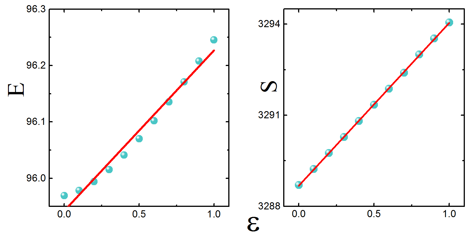
Figure 1: The plots of total energy (left) and EE (right) as a function of $\epsilon$ for the 4d Schwarzschild black hole. We set $N=600$ and $n=150$. The cyan coloured dots are the numerical data and the red line is the best linear fit to the data.

III.2 Reissner-Nordström (RN) black holes

The 4-dimensional Reissner-Nordström black hole is given by the line element in Eq.(5), where $f(\tilde{r})$ is

$$f(\tilde{r})=1-\frac{2M/r_{h}}{\tilde{r}}+\frac{\left(Q/r_{h}\right)^{2}}{\tilde{r}^{2}}$$ (17)

$Q$ is the charge of the black hole. Note that we have rescaled the radius w.r.t the outer horizon ($r_{h}=M+\sqrt{M^{2}-Q^{2}}$). Choosing $q=Q/r_{h}$, we get

$$f(\tilde{r})=1-\frac{(1+q^{2})}{\tilde{r}}+\frac{q^{2}}{\tilde{r}^{2}}$$ (18)

and the black hole temperature in the unit of $r_{h}$ is $T_{BH}=(1-q^{2})/4\pi$.

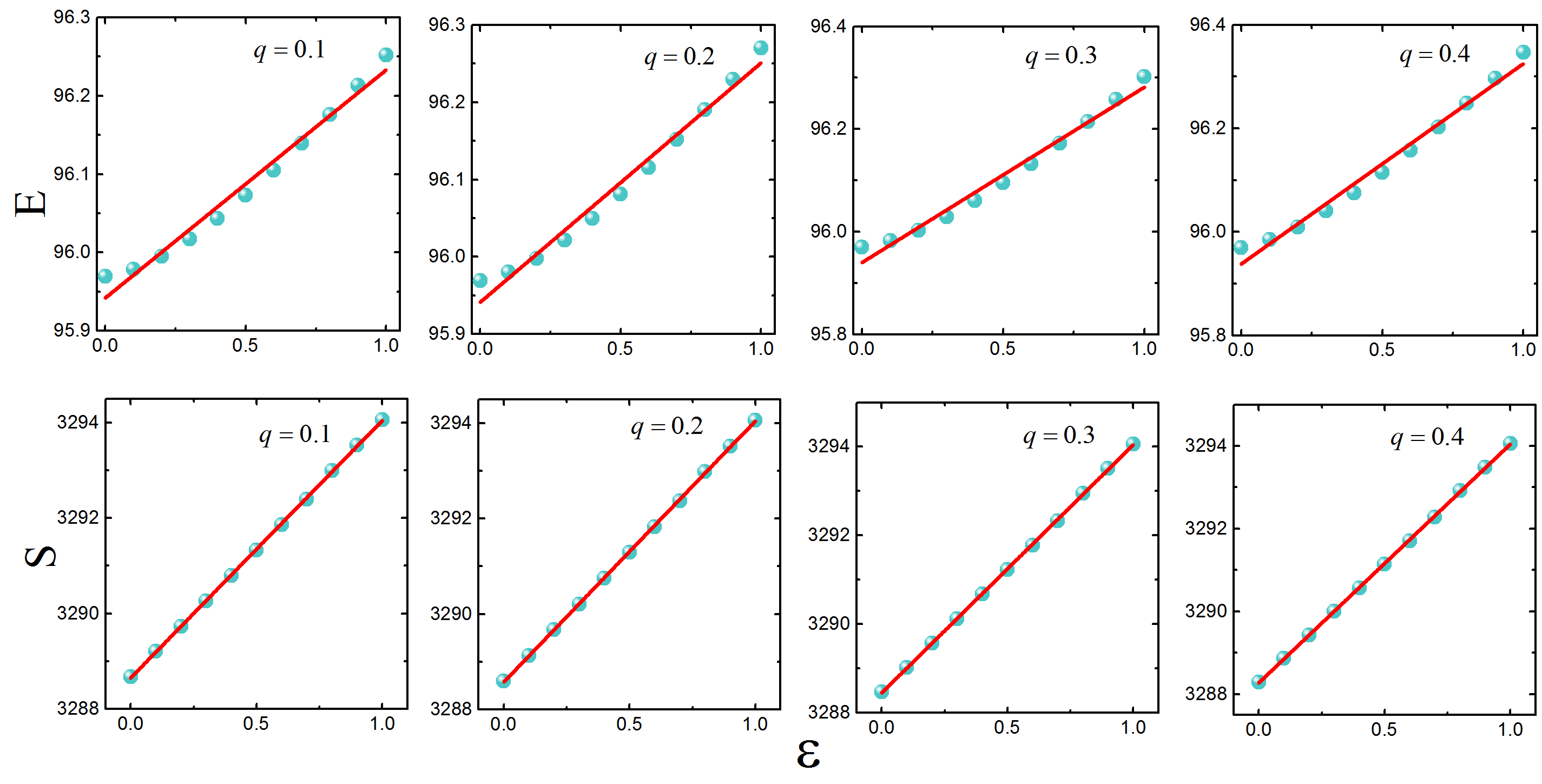
Figure 2: The plots of total energy (top panel) and EE (bottom panel) for as a function of $\epsilon$ for different $q$’s in 4- dimensional Reissner-Nordström black hole. For these, we set $N=600$ and $n=150$. The cyan coloured dots are the numerical data and the red line is the best linear fit to the data.

Note that we have evaluated the entanglement temperature by fixing the charge $q$. For a fixed charge $q$, the first law of black hole mechanics is given by $dE=\left(\kappa/2\pi\right)dA$, where $A$ is the area of the black hole horizon. The energy and EE for different $q$ values have the same profile, which looks exactly like in the previous case and is shown in the middle row in Fig. (2). See Appendix C, for plots for other values of $n$. As given in the table (1), $T_{EE}$ matches with Hawking temperature.

Black hole space time		$\mathbf{T_{BH}}$	$\mathbf{T_{EE}}$
4d-SBH		0.07958	0.07927
4d-RN	$q=0.1$	0.07878	0.07836
	$q=0.2$	0.07639	0.07507
	$q=0.3$	0.07242	0.07501
	$q=0.4$	0.06685	0.06659

Table 1: The table lists entanglement temperature and Hawking temperature (measure in units of $r_{h}$ ) for 4-dimensional Schwarzschild and Reissner-Nordström black hole space times.

IV Conclusions and outlook

In this work, we have given another proof that 4-dimensional black hole entropy can be associated to entropy of entanglement across the horizon by explicitly deriving entanglement temperature. Entanglement temperature is given by the rate of change of the entropy of entanglement across a black hole’s horizon with regard to the system energy. Our new result sheds the light on the interpretation of temperature from entanglement as the Hawking temperature, one more step to understand the black hole thermodynamics from the quantum information theory platform.

Some of the key features of our analysis are: First, while entanglement and energy diverge in the limit of $b\to 0$, the entanglement temperature is a finite quantity. Second, entanglement temperature vanishes for the flat space-time. While the evaluation of the entanglement entropy does not distinguish between the black-hole space-time and flat space-time, entanglement temperature distinguishes the two space-times.

Our analysis also shows that the entanglement entropy satisfies all the properties of the black-hole entropy. First, like the black hole entropy, the entanglement entropy increases and never decreases. Second, the entanglement entropy and the temperature satisfies the first law of black-hole mechanics $dE=T_{EE}\,dS$. We have shown this explicitly for Schwarzschild black-hole and for Reissner-Norstrom black-hole .

It is quite remarkable that in higher dimensional space time the Rényi entropy provides a convergent alternative to the measure of entanglement shanki2013 , however, entanglement temperature will depend on the Rényi parameter. While a physical understanding of the Rényi parameter has emerged baez_renyi_2011 , it is still not clear how to fix the Rényi parameter from first principles progress .

Our analysis throws some light on the emergent gravity paradigm Sakharov2000 ; jacobson95 ; padmanabhan2010 ; Verlinde2011 where gravity is viewed not as a fundamental force. Here we have shown that the information lost across the horizon is related to the black-hole entropy and the laws of black-hole mechanics emerge from the entanglement across the horizon. Since General Relativity reduces gravity to an effect of the curvature of the space-time, it is thought that the microscopic constituents would be the atoms of the space-time itself. Our analysis shows that entanglement across horizons can be used as building blocks of space-time VanRaamsdonk2010-GRG ; VanRaamsdonk2010-IJMP .

One of the unsettling questions in theoretical physics is whether due to Hawking temperature the black-hole has performed a non-unitary transformation on the state of the system aka information loss problem. Our analysis here does not address this for two reasons: (i) Here, we have fixed the radius of the horizon at all times and evaluated the change in the entropy while to address the information loss we need to look at changing horizon radius. (ii) Here, we have used perturbative Hamiltonian, and hence, this analysis fails as the black-hole size shrinks to half-its-size Almheiri2013-JHEP . We hope to report this in future.

While the unitary quantum time-evolution is reversible and retains all information about the initial state, we have shown that the restriction of the degrees of freedom outside the event-horizon at all times leads to temperature analogous to Hawking temperature. Our analysis may have relevance to the eigenstate thermalization hypothesis 1994-srednicki ; rigol2008-nature ; 2012-srednicki ; rahul2015-ARCMP , which we plan to explore.

Appendix A Calculation of Scalar field Hamiltonian in Lemaître coordinate

In this Appendix section, we give details of the derivation of the Hamiltonian (H) upto second order in $\epsilon$. Using the orthogonal properties of the real spherical harmonics $Z_{{}_{lm_{i}}}$, the scalar field action reduces to,

$$\mathcal{S} = \displaystyle\frac{1}{2}\sum_{{}_{l,m_{i}}}\int d\tilde{\tau}\thinspace d\tilde{\xi}\thinspace\tilde{r}^{D}\left[\sqrt{1-f[\tilde{r}]}(\partial_{\tilde{\tau}}\tilde{\Phi}_{lm_{i}})^{2}-\frac{(\partial_{\tilde{\xi}}\tilde{\Phi}_{lm_{i}})^{2}}{\sqrt{1-f[\tilde{r}]}}\displaystyle-\sqrt{1-f[\tilde{r}]}\,\frac{l(l+D-1)}{\tilde{r}^{2}}\tilde{\Phi}_{lm_{i}}^{2}\right]$$ (19)

where $\tilde{r}=r/r_{h},\thinspace\tilde{\xi}=\xi/r_{h},\thinspace\tilde{\tau}=\tau/r_{h},\thinspace\tilde{\Phi}_{lm}=r_{h}\,\Phi_{lm}$ are dimensionless.

Performing the following infinitesimal transformation toms in the above resultant action:

$$\tilde{\tau}\rightarrow\tilde{\tau}^{\prime}=\tilde{\tau}+\epsilon,\,\tilde{\xi}\rightarrow\tilde{\xi}^{\prime}=\tilde{\xi},$$ (20a)

$$\tilde{\Phi}_{lm_{i}}(\tilde{\tau},\tilde{\xi})\rightarrow\tilde{\Phi}^{\prime}_{lm_{i}}(\tilde{\tau}^{\prime},\tilde{\xi^{\prime}})=\tilde{\Phi}_{lm_{i}}(\tilde{\tau},\tilde{\xi}),$$ (20b)

$$\tilde{r}(\tilde{\tau}^{\prime},\tilde{\xi}^{\prime})=\tilde{r}(\tilde{\tau}+\epsilon,\tilde{\xi})$$ (20c)

The action in Eq. (19) becomes,

$$\mathcal{S} \simeq \displaystyle\frac{1}{2}\sum_{{}_{l,m_{i}}}\int d\tilde{\tau}\thinspace d\tilde{\xi}\thinspace\left(\tilde{r}+\epsilon h_{1}+\epsilon^{2}h_{2}/2\right)^{D}\left[\left(1-f-\epsilon h_{1}\frac{\partial f}{\partial\tilde{r}}-\frac{\epsilon^{2}}{2}\left[h_{2}\frac{\partial f}{\partial\tilde{r}}+h_{1}^{2}\frac{\partial^{2}f}{\partial\tilde{r}^{2}}\right]\right)^{1/2}(\partial_{\tilde{\tau}}\tilde{\Phi}_{lm_{i}})^{2}\right.$$ (21)

$$\left.-\left(1-f-\epsilon h_{1}\frac{\partial f}{\partial\tilde{r}}-\frac{\epsilon^{2}}{2}\left[h_{2}\frac{\partial f}{\partial\tilde{r}}+h_{1}^{2}\frac{\partial^{2}f}{\partial\tilde{r}^{2}}\right]\right)^{-1/2}(\partial_{\tilde{\xi}}\tilde{\Phi}_{lm_{i}})^{2}-\frac{l(l+D-1)}{\left(\tilde{r}+\epsilon h_{1}+\epsilon^{2}h_{2}/2\right)^{2}}\right.$$

$$\left.\times\left(1-f-\epsilon h_{1}\frac{\partial f}{\partial\tilde{r}}-\frac{\epsilon^{2}}{2}\left[h_{2}\frac{\partial f}{\partial\tilde{r}}+h_{1}^{2}\frac{\partial^{2}f}{\partial\tilde{r}^{2}}\right]\right)^{1/2}\tilde{\Phi}_{lm_{i}}^{2}\right]$$

where $h_{1}=\displaystyle\frac{\partial\tilde{r}}{\partial\tilde{\tau}}~{}~{}\mbox{and}~{}~{}h_{2}=\displaystyle\frac{\partial^{2}\tilde{r}}{\partial\tilde{\tau}^{2}}$.

Using the relation between the Lemaître coordinates L&L-2

$$\xi-\tau=\int\frac{dr}{\sqrt{1-f[r(\tau,\xi)]}}$$ (22)

gives the following expression,

$$h_{1}=-\sqrt{1-f},~{}~{}h_{2}=\frac{-1}{2}\frac{\partial f}{\partial\tilde{r}},~{}~{}\frac{d\tilde{\xi}}{d\tilde{r}}|_{\mbox{con.}\tilde{\tau}}=\frac{1}{\sqrt{1-f}}$$ (23)

The Hamiltonian $(H)$ corresponding to the above Lagrangian is

$$H\simeq\displaystyle\frac{1}{2}\sum_{{}_{l,m_{i}}}\int d\tilde{\xi}\left[\tilde{\Pi}_{lm_{i}}^{2}+\frac{g_{{}_{1}}^{D}}{g_{{}_{2}}}\left(\partial_{\tilde{\xi}}\frac{\tilde{\chi}_{{}_{lm_{i}}}}{g_{{}_{1}}^{D/2}\sqrt{g_{{}_{2}}}}\right)^{2}+\frac{l(l+D-1)}{g_{{}_{1}}^{2}}\tilde{\chi}_{{}_{lm_{i}}}^{2}\right]$$ (24)

where

$$g_{{}_{1}}=\tilde{r}+\epsilon h_{1}+\epsilon^{2}h_{2}/2,~{}~{}g_{{}_{2}}=\sqrt{1-f-\epsilon h_{1}\frac{\partial f}{\partial\tilde{r}}-\frac{\epsilon^{2}}{2}\left[h_{2}\frac{\partial f}{\partial\tilde{r}}+h_{1}^{2}\frac{\partial^{2}f}{\partial\tilde{r}^{2}}\right]},~{}~{}\tilde{\chi}_{{}_{lm_{i}}}=g_{{}_{1}}^{D/2}\sqrt{g_{{}_{2}}}\tilde{\Phi}_{lm_{i}}$$ (25)

and $\tilde{\Pi}_{lm_{i}}$ is the canonical conjugate momenta corresponding to the field $\tilde{\chi}_{lm_{i}}$.

Upon quantization, $\tilde{\Pi}_{lm_{i}}$ and $\tilde{\chi}_{lm_{i}}$ satisfy the usual canonical commutation relation:

$$\left[\tilde{\chi}_{lm_{i}}\left({\tilde{\xi},\tilde{\tau}}\right),\tilde{\Pi}_{l^{\prime}m^{\prime}_{i}}\left({\tilde{\xi^{\prime}},\tilde{\tau}}\right)\right]=i\delta_{ll^{\prime}}\delta_{m_{i}m^{\prime}_{i}}\delta\left(\tilde{\xi}-\tilde{\xi^{\prime}}\right)$$ (26)

Using relations (23) and expanding the Hamiltonian up to second order in $\epsilon$, we get,

$$H \simeq\displaystyle\frac{1}{2}\sum_{{}_{l,m_{i}}}\displaystyle\int_{\displaystyle\tilde{\tau}}^{\infty}d\tilde{r}\left[\pi^{2}_{lm_{i}}+\tilde{r}^{D}\displaystyle\frac{\left(1-\epsilon H_{{}_{1}}-\epsilon^{2}H_{{}_{2}}\right)^{D}}{\left(\displaystyle 1+\epsilon H_{{}_{3}}-\epsilon^{2}H_{{}_{4}}\right)^{1/2}}\left[\partial_{\tilde{r}}\frac{\sigma_{lm_{i}}}{\tilde{r}^{D/2}\left(1-\epsilon H_{{}_{1}}-\epsilon^{2}H_{{}_{2}}\right)^{D/2}\left(\displaystyle 1+\epsilon H_{{}_{3}}-\epsilon^{2}H_{{}_{4}}\right)^{1/4}}\right]^{2}\right.$$ (27)

$$\left.\displaystyle+\frac{l(l+D-1)}{\tilde{r}^{2}\left(1-\epsilon H_{{}_{1}}-\epsilon^{2}H_{{}_{2}}\right)^{2}}\sigma^{2}_{lm_{i}}\right]$$

The Hamiltonian in Eq. (27)is of the form

$$H\simeq H_{{}_{0}}+\epsilon V_{{}_{1}}+\epsilon^{2}V_{{}_{2}}$$ (28)

where $H_{{}_{0}}$ is the unperturbed scalar field Hamiltonian in the flat space-time, $V_{{}_{1}}\mbox{and}\,V_{{}_{2}}$ are the perturbed parts of the Hamiltonian given by;

$$H_{{}_{0}} = \displaystyle\frac{1}{2}\sum_{{}_{l,m_{i}}}\displaystyle\int_{\displaystyle\tilde{\tau}}^{\infty}d\tilde{r}\left[\pi^{2}_{lm_{i}}+\tilde{r}^{D}\displaystyle\left[\partial_{\tilde{r}}\displaystyle\frac{\sigma_{lm_{i}}}{\tilde{r}^{D/2}}\right]^{2}+\frac{l(l+D-1)}{\tilde{r}^{2}}\sigma^{2}_{lm_{i}}\right]$$ (29)

$$V_{{}_{1}} = \displaystyle\frac{1}{2}\sum_{{}_{l,m_{i}}}\displaystyle\int_{\displaystyle\tilde{\tau}}^{\infty}d\tilde{r}\left[\frac{\left(-D\,\sigma_{lm_{i}}+2\tilde{r}\,\sigma^{\prime}_{lm_{i}}\right)\left(DH_{3}\,\sigma_{lm_{i}}-2\tilde{r}H_{3}\,\sigma^{\prime}_{lm_{i}}+2D\tilde{r}H_{1}^{\prime}\,\sigma_{lm_{i}}-\tilde{r}H_{3}^{\prime}\,\sigma_{lm_{i}}\right)}{4\tilde{r}^{2}}\right.$$ (30)

$$\left.\displaystyle+\frac{2l(l+D-1)H_{{}_{1}}}{\tilde{r}^{2}}\sigma^{2}_{lm_{i}}\right]$$

$$V_{{}_{2}} = \displaystyle\frac{1}{2}\sum_{{}_{l,m_{i}}}\displaystyle\int_{\displaystyle\tilde{\tau}}^{\infty}d\tilde{r}\left[\left(H^{2}_{3}+H_{4}\right)\,\sigma^{\prime 2}_{lm_{i}}+\left(-\frac{DH^{2}_{3}}{\tilde{r}}-\frac{DH_{4}}{\tilde{r}}+DH_{1}H_{1}^{\prime}-DH_{3}H_{1}^{\prime}+DH_{2}^{\prime}+H_{3}H_{3}^{\prime}+\frac{1}{2}H_{4}^{\prime}\right)\,\sigma^{\prime}_{lm_{i}}\sigma_{lm_{i}}\right.$$ (31)

$$\left.+\left(\frac{l(l+D-1)\left(3H^{2}_{1}+2H_{2}\right)}{\tilde{r}^{2}}+\frac{D^{2}H_{3}^{2}}{4\tilde{r}^{2}}+\frac{D^{2}H_{4}}{4\tilde{r}^{2}}-\frac{D^{2}H_{1}H_{1}^{\prime}}{2\tilde{r}}+\frac{D^{2}H_{3}H_{1}^{\prime}}{2\tilde{r}}+\frac{1}{4}D^{2}H_{1}^{\prime 2}-\frac{D^{2}H_{2}^{\prime}}{2\tilde{r}}\right.\right.$$

$$\left.\left.-\frac{DH_{3}H_{3}^{\prime}}{2\tilde{r}}-\frac{1}{4}DH_{1}^{\prime}H_{3}^{\prime}+\frac{1}{16}H_{3}^{\prime 2}-\frac{dH_{4}^{\prime}}{4\tilde{r}}\right)\,\sigma^{2}_{lm_{i}}\right]$$

where

$$H_{{}_{1}}=\displaystyle\frac{\sqrt{1-f}}{\tilde{r}},\quad H_{{}_{2}}=\frac{1}{4\tilde{r}}\frac{\partial f}{\partial\tilde{r}},\quad H_{{}_{3}}=\displaystyle\frac{1}{\sqrt{1-f}}\frac{\partial f}{\partial\tilde{r}},\quad H_{{}_{4}}=\frac{-1}{4(1-f)}\left(\frac{\partial f}{\partial\tilde{r}}\right)^{2}+\frac{1}{2}\frac{\partial^{2}f}{\partial\tilde{r}^{2}}$$ (32)

and the redefined field operators are

$$\tilde{\Pi}_{lm_{i}}=\frac{\pi_{lm_{i}}}{\left(1-f\right)^{1/4}}\quad\mbox{and}\quad\tilde{\chi}_{lm_{i}}=\frac{\sigma_{lm_{i}}}{\left(1-f\right)^{1/4}}$$ (33)

such that they satisfy the following canonical commutation relation

$$\left[\pi_{lm_{i}}(\tilde{r},\tilde{\tau}),\sigma_{l^{\prime}m^{\prime}_{i}}(\tilde{r}^{\prime},\tilde{\tau})\right]=i\delta_{ll^{\prime}}\delta_{m_{i}m^{\prime}_{i}}\delta(\tilde{r}-\tilde{r}^{\prime})$$ (34)

The Hamiltonian $H$ in Eq. (28) is mapped to a system of $N$ coupled time independent harmonic oscillators (HO) with non-periodic boundary conditions. The interaction matrix elements of the Hamiltonian can be found in the Ref.dropbox . The total internal energy (E) and the entanglement entropy ($S_{\alpha}$) for the ground state of the HO’s is computed numerically as a function of $\epsilon$ by using central difference scheme.

Appendix B Central Difference discretization

This is one of the effective method for finding the approximate value for derivative of a function in the neighbourhood of any discrete point, $x_{i}=x_{0}+i\;h$,with unit steps of $h$. The Taylor expansion of the function about the point $x_{0}$ in the forward and backward difference scheme is given respectively by,

$$f(x+h)=f(x)+\frac{hf^{\prime}(x)}{1!}+\frac{h^{2}f^{\prime\prime}(x)}{2!}+......$$ (35)

$$f(x-h)=f(x)-\frac{hf^{\prime}(x)}{1!}+\frac{h^{2}f^{\prime\prime}(x)}{2!}-.......$$ (36)

which implies,

$$f^{\prime}(x) = \frac{f(x+h)-f(x-h)}{2h}+O(h^{2})$$ (37)

$$f^{\prime\prime}(x) = \frac{f(x+h)-2f(x)+f(x-h)}{h^{2}}+O(h^{2})$$ (38)

$$f^{\prime\prime\prime}(x) = \frac{f(x+2h)-2f(x+h)+2f(x-h)+f(x-2h)}{2h^{3}}+O(h^{2})$$ (39)

Appendix C Plots of internal energy and EE as a function of $\epsilon$ for different black hole space-times

In this section of Appendix, we give plots of EE for different black hole space-times;

Figure 3: Plots of the EE as function of $\epsilon$ for the 4-d Schwarzschild black hole with $N=300$, $n=50,80,100$, and $130$, respectively. The blue dots are the numerical data and the red line is the best linear fit to the data.

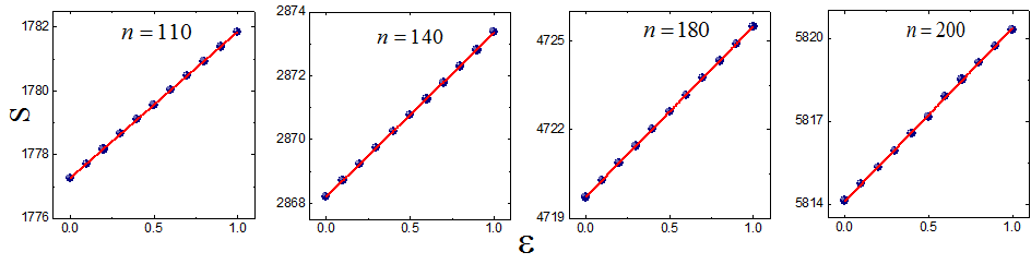
Figure 4: Plots of the EE as function of $\epsilon$ for the 4-d Schwarzschild black hole with $N=400$, $n=110,140,180$, and $200$ respectively. The blue dots are the numerical data and the red line is the best linear fit to the data.

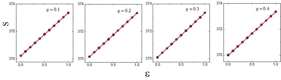
Figure 5: Plots of the EE of 4-d R-N black hole in terms of $\epsilon$ for different $q$’s with $N=300$, and $n=50$. The blue dots are the numerical data and the red line is the best linear fit to the data.

References

- (1) G. D. Birkhoff, “Proof of a Recurrence Theorem for Strongly Transitive Systems,” Proceedings of the National Academy of Science 17 (Dec., 1931) 650–655.
- (2) J. V. Neumann, “Proof of the quasi-ergodic hypothesis,” Proceedings of the National Academy of Sciences 18 no. 1, (1932) 70–82.
- (3) L. Boltzmann, Lectures on Gas Theory. Dover Books on Physics. Dover Publications, 2011.
- (4) L. D. Landau and E. M. Lifshitz, Statistical Physics, vol. V of Course of Theoretical Physics. Elsevier, 3 ed., 1980.
- (5) A. Wehrl, “General properties of entropy,” Rev. Mod. Phys. 50 no. 2, (Apr., 1978) 221–260.
- (6) Kinoshita Toshiya, Wenger Trevor, and Weiss David S., “A quantum Newton’s cradle,” Nature 440 no. 7086, (Apr, 2006) 900?903.
- (7) Esteve J., Gross C., Weller A., Giovanazzi S., and Oberthaler M. K., “Squeezing and entanglement in a Bose-Einstein condensate,” Nature 455 no. 7217, (Oct, 2008) 1216–1219.
- (8) D. A. Smith, M. Gring, T. Langen, M. Kuhnert, B. Rauer, R. Geiger, T. Kitagawa, I. Mazets, E. Demler, and J. Schmiedmayer, “Prethermalization revealed by the relaxation dynamics of full distribution functions,” New Journal of Physics 15 no. 7, (2013) 075011.
- (9) V. I. Yukalov, “Bose-einstein condensation and gauge symmetry breaking,” Laser Physics Letters 4 no. 9, (2007) 632.
- (10) A. Osterloh, L. Amico, G. Falci, and R. Fazio, “Scaling of entanglement close to a quantum phase transition,” Nature 416 (Dec, 2002) 608.
- (11) L.-A. Wu, M. S. Sarandy, and D. A. Lidar, “Quantum phase transitions and bipartite entanglement,” Phys. Rev. Lett. 93 (Dec, 2004) 250404.
- (12) J. von Stecher, E. Demler, M. D. Lukin, and A. M. Rey, “Probing interaction-induced ferromagnetism in optical superlattices,” New Journal of Physics 12 no. 5, (2010) 055009.
- (13) J. Dinerman and L. F. Santos, “Manipulation of the dynamics of many-body systems via quantum control methods,” New Journal of Physics 12 no. 5, (2010) 055025.
- (14) L. Seth, “Quantum Thermodynamics: Excuse our ignorance,” Nature Physics 2 no. 11, (Nov, 2006) 727–728.
- (15) F. G. S. L. Brandao and M. B. Plenio , “Entanglement theory and the second law of thermodynamics,” Nature Physics 4 no. 11, (Nov, 2008) 873–877.
- (16) M. Horodecki, “Quantum entanglement: Reversible path to thermodynamics,” Nature Physics 4 no. 11, (Nov, 2008) 833–834.
- (17) S. Popescu and D. Rohrlich, “Thermodynamics and the measure of entanglement,” Phys. Rev. A 56 (1997) R3319–R3321.
- (18) V. Vedral and M. B. Plenio, “Entanglement measures and purification procedures,” Phys. Rev. A 57 (Mar, 1998) 1619–1633.
- (19) M. B. Plenio and V. Vedral, “Teleportation, entanglement and thermodynamics in the quantum world,” Contemporary Physics 39 no. 6, (Nov., 1998) 431–446.
- (20) M. Srednicki, “Chaos and quantum thermalization,” Phys. Rev. E 50 (1994) 888–901.
- (21) Rigol Marcos, Dunjko Vanja, and Olshanii Maxim, “Thermalization and its mechanism for generic isolated quantum systems,” Nature 452 no. 7189, (Apr, 2008) 854?–858.
- (22) M. Rigol and M. Srednicki, “Alternatives to eigenstate thermalization,” Phys. Rev. Lett. 108 (2012) 110601.
- (23) R. Nandkishore and D. A. Huse, “Many-body localization and thermalization in quantum statistical mechanics,” Annual Review of Condensed Matter Physics 6 no. 1, (2015) 15–38.
- (24) L. Bombelli, R. K. Koul, J. Lee, and R. D. Sorkin, “Quantum source of entropy for black holes,” Phys. Rev. D 34 (Jul, 1986) 373–383.
- (25) M. Srednicki, “Entropy and area,” Phys. Rev. Lett. 71 (Aug, 1993) 666–669.
- (26) J. Eisert and M. Cramer, “Single-copy entanglement in critical quantum spin chains,” Phys. Rev. A 72 (Oct, 2005) 042112.
- (27) S. Das and S. Shankaranarayanan, “How robust is the entanglement entropy-area relation?,” Phys. Rev. D 73 (Jun, 2006) 121701.
- (28) S. Das, S. Shankaranarayanan, and S. Sur, Black hole entropy from entanglement: A review edited by M. Everett and L. Pedroza, vol. 268 of Horizons in World Physics. Nova Science Publishers,, New York, 2009. page 211.
- (29) S. N. Solodukhin, “Entanglement Entropy of Black Holes,” Living Reviews in Relativity 14 (2011) .
- (30) S. L. Braunstein, S. Das, and S. Shankaranarayanan, “Entanglement entropy in all dimensions,” Journal of High Energy Physics 2013 no. 7, (2013) 1–9.
- (31) S. W. Hawking, “Particle creation by black holes,” Communications in Mathematical Physics 43 (1975) 199–220.
- (32) R. Horodecki, P. Horodecki, M. Horodecki, and K. Horodecki, “Quantum entanglement,” Rev. Mod. Phys. 81 (Jun, 2009) 865–942.
- (33) J. Eisert, M. Cramer, and M. B. Plenio, “Colloquium : Area laws for the entanglement entropy,” Rev. Mod. Phys. 82 (Feb, 2010) 277–306.
- (34) P. Calabrese and J. L. Cardy, “Entanglement entropy and quantum field theory,” Journal of Statistical Mechanics: Theory and Experiment 0406 (2004) P06002.
- (35) K. Mallayya, R. Tibrewala, S. Shankaranarayanan, and T. Padmanabhan, “Zero modes and divergence of entanglement entropy,” Phys. Rev. D 90 (Aug, 2014) 044058.
- (36) S. Mukohyama, M. Seriu, and H. Kodama, “Thermodynamics of entanglement in schwarzschild spacetime,” Phys. Rev. D 58 (Jul, 1998) 064001.
- (37) L. D. Landau and E. M. Lifshitz, The Classical Theory of Fields, vol. II of Course of Theoretical Physics. Butterworth-Heinemann, 4 ed., 1975.
- (38) D. J. Toms, The Schwinger action principle and effective action. Cambridge monographs on mathematical physics. Cambridge Univ. Press, Cambridge, 2007.
- (39) H. Sakaguchi, “Renyi entropy and statistical mechanics,” Progress of Theoretical Physics 81 no. 4, (1989) 732–737.
- (40) Click on the following ‘Dropbox’ link for more details on MATLAB codes that use for the numerical study reported in the paper, https://www.dropbox.com/sh/wxmq02qxg6m3pbm/AABEE-k4MMow7FJj_JHgfrV_a?dl=0.
- (41) J. C. Baez, “Rényi entropy and free energy,” arXiv:1102.2098 [quant-ph].
- (42) Work under progress.
- (43) A. D. Sakharov, “Vacuum quantum fluctuations in curved space and the theory of gravitation,” General Relativity and Gravitation 32 no. 2, (2000) 365–367.
- (44) T. Jacobson, “Thermodynamics of spacetime: The einstein equation of state,” Phys. Rev. Lett. 75 (Aug, 1995) 1260–1263.
- (45) T. Padmanabhan, “Thermodynamical aspects of gravity: new insights,” Reports on Progress in Physics 73 no. 4, (Apr., 2010) 046901.
- (46) E. Verlinde, “On the origin of gravity and the laws of newton,” Journal of High Energy Physics 2011 no. 4, (2011) .
- (47) M. Van Raamsdonk, “Building up spacetime with quantum entanglement,” General Relativity and Gravitation 42 no. 10, (2010) 2323–2329.
- (48) M. Van Raamsdonk, “Building up space?time with quantum entanglement,” International Journal of Modern Physics D 19 no. 14, (2010) 2429–2435.
- (49) A. Almheiri, D. Marolf, J. Polchinski, and J. Sully, “Black holes: complementarity or firewalls?,” Journal of High Energy Physics 2013 no. 2, (2013) 1–20.