Combined shared and distributed memory ab-initio computations of molecular-hydrogen systems in the correlated state: process pool solution and two-level parallelism

Abstract

An efficient computational scheme devised for investigations of ground state properties of the electronically correlated systems is presented. As an example, $(H_{2})_{n}$ chain is considered with the long-range electron-electron interactions taken into account. The implemented procedure covers: (i) single-particle Wannier wave-function basis construction in the correlated state, (ii) microscopic parameters calculation, and (iii) ground state energy optimization. The optimization loop is based on highly effective process-pool solution – specific root–workers approach. The hierarchical, two-level parallelism was applied: both shared (by use of Open Multi-Processing) and distributed (by use of Message Passing Interface) memory models were utilized. We discuss in detail the feature that such approach results in a substantial increase of the calculation speed reaching factor of $300$ for the fully parallelized solution. The elaborated in detail scheme reflects the situation in which the most demanding task is the single-particle basis optimization.

I Physical Motivation: Exact Diagonalization + ab Initio Method

Electronically correlated systems are important both from the point of view of their unique physical properties and from nontrivial computational methods developed to determine them. The latter cover methods based on the Density Functional Theory (DFT) with the energy functional enriched by the correlation terms – the on-site repulsion $U$ in the Hubbard model Himmetoglu et al. (2014) and the Hund’s rule term in the case of orbital degeneracy. Often, they are incorporated into either DFT or the Dynamic Mean Field Theory (DMFT) approach supplemented with the LDA-type calculations (see e.g. Karolak et al. (2010)). On the other hand, the Configuration-Interaction (CI) method does not suffer from the well–known double counting problemHimmetoglu et al. (2014); Karolak et al. (2010), inherent in the DFT+U or LDA+DMFT methods. Another approach, similar in its spirit to the CI method, formulated as a combination of the first- and second quantization (FQ, SQ respectively) formalisms was elaborated in our group in the last decade and termed the Exact Diagonalization Ab Intito (EDABI) approach Spałek et al. (2000, 2007). This method allows for a natural incorporation of the correlation effects consistently by the advantages of using the SQ language so that the double-counting problem does not arise at all. Also, by construction, it includes the Pauli principle for the fermionic systems. In contrast to CI the EDABI approach avoids any direct dealing with the many–body wave function expressed via a linear combination of the Slater determinants Surjan (1989). Instead, it is based on the many–particle quantum states constructed in the occupation number representation Surjan (1989) – standard procedure for the SQ formulated problems.

The application of EDABI was found promising in view of research devoted to the hydrogen molecular systems with inclusion of interelectronic correlations Kądzielawa et al. (2014), nano-clusters Rycerz (2003), and to atomic hydrogen metallization Kądzielawa et al. (2013). As the many–particle state is explicitly written in the occupation-number representation (Fock space), the starting Hamiltonian is formulated in the SQ language. Electronic correlations are then automatically included in the modeled system. However, in the Hubbard–like starting Hamiltonians Hubbard (1963); Gutzwiller (1963, 1965); Kanamori (1963) the knowledge of microscopic parameters, such as the on-site energy, the intersite hoppings, and the Coulomb repulsion magnitudes are regarded as input information. These parameters are often estimated indirectly. With this limitation, specific phase-diagrams are constructed and the phase boundaries of interest are determined as a function of those microscopic parameters which are not directly measurable (cf. e.g. Zegrodnik and Spałek (2012); Zegrodnik et al. (2014); Wysokiński et al. (2014)). In EDABI we take a different route: relatively simple and small systems are to be described consistently in the sense that the microscopic parameters are obtained explicitly as an output of an appropriate ab-initio variational procedure. Therefore, the EDABI approach should be regarded as an ab–initio method but with the single-particle wave functions being determined self-consistently in the correlated state. In this manner, the problem solution is reversed with respect to that in either LDA+U or LDA+DMFT. Namely, we first formulate the Hamiltonian and diagonalize it in SQ formalism and determine the single-particle wave function only as a second step. However realistic, such an approach to the electronically correlated systems implies a substantially greater computational complexity, since the variational optimization consists of (i) microscopic parameters calculation and (ii) concomitant Hamiltonian-matrix diagonalization. We address here the issue (i) presenting how the modern High Performance Computing (HPC) cluster architecture can be utilized in the context, where the number of microscopic parameters is substantial if not large, and their calculation is one of the potential bottlenecks in the whole computational procedure. We also provide an example how a many-body problem at hand may be supplemented with the two-level parallelism in an intuitive manner. We do not discuss either the methodology related to the point (ii) or to its algorithmic aspect or else, to technical opportunities provided by e.g. recent fast development of Graphic Processing Units (GPU) computational techniques that are also in the area of interest Siro and Harju (2012); Wendt et al. (2011). Nonetheless, as it becomes clear below, heterogeneous solutions are also easily applicable in our scheme.

The structure of the paper is as follows. In Sec. II we describe briefly the EDABI method (cf. Appendix A for details) and emphasize the computational complexity aspects. Next, in Sec. III, we show how the process–pool concept enhanced by the two-level parallelism forms a natural solution. In Sec. IV we present the outcome of its implementation: results of calculations carried out for $(H_{2})_{n}$ exemplary system and discuss the achieved speed–up when compared to the reference single CPU computations. In Appendix B we discuss the convergence of our model for the case of infinite systems.

II Computational method - EDABI

As stated in the foregoing Section, the computational method considered here is based on the EDABI method, comprehensive description of which can be found e.g. in Spałek et al. (2000). It allows for consideration of realistic, electronically–correlated nanosystems within the framework of the combined first– and second-quantization formalisms. Below we sketch this method (for details see Appendix A).

II.1 Second-quantization aspect

For the purpose of calculating the ground-state energy of given system we start with the second-quantization language Dirac (1927); Fock (1932); Surjan (1989); Fetter and Walecka (2003). We introduce the fermonic anihilator(creator) $\hat{c}^{(\dagger)}_{i\sigma}$ algebra by imposing the anticommutation relations among them, namely

$$\{\hat{c}^{\dagger}_{{i}\sigma},\hat{c}^{\dagger}_{{j}\sigma^{\prime}}\}\equiv\{\hat{c}_{{i}\sigma},\hat{c}_{{j}\sigma^{\prime}}\}\equiv 0\ \ \ \text{and}\ \ \{\hat{c}^{\dagger}_{{i}\sigma},\hat{c}_{{j}\sigma^{\prime}}\}\equiv\delta_{ij}\delta_{\sigma\sigma^{\prime}},$$ (1)

where $i$ and $j$ denote sites (nodes) of a fixed lattice, $\sigma,\ \sigma^{\prime}=\pm 1$ are the spin quantum number, and the anticommutator is $\{A,B\}\equiv AB+BA$.

We represent the many-particle basis states $\{\left|\Phi_{k}\right\rangle\}$ on the lattice of $\Lambda$ sites in the Fock space Fock (1932) in the following manner

$$\left|\Phi_{k}\right\rangle= \prod_{i\in\Omega_{\uparrow k}}\hat{c}^{\dagger}_{{i}\uparrow}\prod_{j\in\Omega_{\downarrow k}}\hat{c}^{\dagger}_{{j}\uparrow}\left|0\right\rangle,$$ (2)

where $\Omega_{\uparrow k}$ and $\Omega_{\downarrow k}$ are the subsets of sites occupied by fermions with $\Lambda_{\uparrow}$ and $\Lambda_{\downarrow}$ particles respectively, and $\left|0\right\rangle$ is the vacuum state (with no particles), with $\left\langle 0\vphantom{0}\right|\left.0\vphantom{0}\right\rangle\equiv 1$. Explicitly,

$$\left|\Phi\right\rangle= \underbrace{\left|0,1,\dots,1\right\rangle}_{\text{spin }\uparrow}\otimes\underbrace{\left|1,0,\dots,1\right\rangle}_{\text{spin }\downarrow}=$$ (3)

$$= \hat{c}^{\dagger}_{{2}\uparrow}\cdots\hat{c}^{\dagger}_{{\Lambda}\uparrow}\hat{c}^{\dagger}_{{1}\downarrow}\cdots\hat{c}^{\dagger}_{{\Lambda}\downarrow}\left|0\right\rangle.$$

With this concrete (occupation-number) representation of an abstract Fock space we define next the microscopic Hamiltonian of our interacting system of fermions.

II.2 Definition of the physical problem

We take the real-space representation with the starting field operators in the form

$$\hat{\Psi}^{\phantom{\dagger}}_{\sigma}(\mathbf{r})=\sum_{i}w_{i}(\mathbf{r})\chi_{\sigma}\hat{c}_{{i}\sigma},$$ (4)

where $w_{i}(\mathbf{r})$ is the single-particle wave function for fermion (e.g. electron) located on $i$-th site, $\chi_{\sigma}$ is the spin wave function ($\sigma=\pm 1$) with global spin quantization axis ($z$-axis). In general, the many-particle Hamiltonian is defined in the form

$$\hat{\mathcal{H}}= \sum_{\sigma}\int d^{3}r\hat{\Psi}^{{\dagger}}_{\sigma}(\mathbf{r})\hat{\mathcal{H}}_{1}(\mathbf{r})\hat{\Psi}^{\phantom{\dagger}}_{\sigma}(\mathbf{r})$$ (5)

$$+\frac{1}{2}\sum_{\sigma\sigma^{\prime}}\iint d^{3}rd^{3}r^{\prime}\hat{\Psi}^{{\dagger}}_{\sigma}(\mathbf{r})\hat{\Psi}^{{\dagger}}_{\sigma^{\prime}}(\mathbf{r}^{\prime})\hat{V}(\mathbf{r}-\mathbf{r}^{\prime})\hat{\Psi}^{\phantom{\dagger}}_{\sigma^{\prime}}(\mathbf{r}^{\prime})\hat{\Psi}^{\phantom{\dagger}}_{\sigma}(\mathbf{r}),$$

where $\hat{\mathcal{H}}_{1}$ is the (spin-independent) Hamiltonian for a single particle in the milieu of all other particles and $\hat{V}(\mathbf{r}-\mathbf{r}^{\prime})$ is the interaction energy for a single pair. For the modeling purposes we assume that $\hat{\mathcal{H}}_{1}$ is expressed in the atomic units ($\hbar=e^{2}/2=2m_{e}=1$, where $e$ is the charge of an electron and $m_{e}$ is its mass) and expresses the particle kinetic energy and the attractive interaction with the protons located at $\{\mathbf{R}_{i}\}$, i.e.,

$$\hat{\mathcal{H}}_{1}(\mathbf{r}) \overset{a.u.}{=}-\nabla^{2}-\sum_{i=1}^{N_{S}}\frac{2}{|\mathbf{R_{i}}-\mathbf{r}|},$$ (6)

where $N_{S}$ is the number of sites, whereas

$$\hat{V}(\mathbf{r}-\mathbf{r}^{\prime}) \overset{a.u.}{=}\frac{2}{|\mathbf{r}-\mathbf{r^{\prime}}|},$$ (7)

represents the Coulomb repulsive interaction between them. Substituting (4) into (5) we obtain the explicit second-quantized form of the Hamiltonian Fetter and Walecka (2003); Surjan (1989) i.e.,

$$\mathcal{H}=\sum\limits_{ij}\sum\limits_{\sigma}t_{ij}\hat{c}^{\dagger}_{{i}\sigma}\hat{c}_{{j}\sigma}+\sum\limits_{ijkl}\sum\limits_{\sigma,\sigma^{\prime}}V_{ijkl}\hat{c}^{\dagger}_{{i}\sigma}\hat{c}^{\dagger}_{{j}\sigma^{\prime}}\hat{c}_{{l}\sigma^{\prime}}\hat{c}_{{k}\sigma},$$ (8)

where $t_{ij}$ and $V_{ijkl}$ are integrals associated with the one- and two-body operators respectively

$$t_{ij} \equiv\left\langle w_{i}(\mathbf{r})\vphantom{\hat{\mathcal{H}}_{1}w_{j}(\mathbf{r})}\right|\hat{\mathcal{H}}_{1}\left|w_{j}(\mathbf{r})\vphantom{w_{i}(\mathbf{r})\hat{\mathcal{H}}_{1}}\right\rangle$$ (9a)

$$=\int d^{3}r\ w_{i}^{*}(\mathbf{r})\hat{\mathcal{H}}_{1}(\mathbf{r})w_{j}(\mathbf{r}),$$

$$V_{ijkl} \equiv\left\langle w_{i}(\mathbf{r})w_{j}(\mathbf{r^{\prime}})\vphantom{\hat{V}w_{k}(\mathbf{r})w_{l}(\mathbf{r}^{\prime})}\right|\hat{V}\left|w_{k}(\mathbf{r})w_{l}(\mathbf{r}^{\prime})\vphantom{w_{i}(\mathbf{r})w_{j}(\mathbf{r^{\prime}})\hat{V}}\right\rangle$$ (9b)

$$=\iint d^{3}rd^{3}r^{\prime}\ w_{i}^{*}(\mathbf{r})w_{j}^{*}(\mathbf{r}^{\prime})\hat{V}(\mathbf{r}-\mathbf{r}^{\prime})w_{k}(\mathbf{r})w_{l}(\mathbf{r}^{\prime}).$$

The first term contains the single-particle part composed of the atomic energy $\epsilon_{i}\equiv t_{ii}$, as well as expresses the kinetic (hopping) part with $t_{ij}$ ($i\neq j$) being the so-called hopping integral. The second expression contains intraatomic (intrasite) part of the interaction between the particles ($U_{i}\equiv V_{iiii}$ – the so-called Hubbard interaction), and the intersite (interatomic) interaction ($K_{ij}\equiv V_{ijij}$ – the last important term for the purposes here). A remark is in place here: when the single-particle basis $\{w_{i}\}$ is assumed as real, the last two two-body interaction terms are the exchange-correlation energy ($J_{ij}\equiv V_{ijji}$) and the so-called correlated hopping ($V_{ij}\equiv V_{ijjj}$).

The Hamiltonian (5), with inclusion of all the two-site terms only, can be rewritten in the following form, with the microscopic parameters contained in an explicit manner, i.e.,

$$\hat{\mathcal{H}} =\sum_{i,\sigma}\epsilon_{i}\hat{n}_{{i\sigma}}+\frac{1}{2}\sum_{\sigma,i\neq j}t_{ij}\hat{c}^{\dagger}_{{i\sigma}}\hat{c}_{{j\sigma}}+\frac{1}{2}\sum_{i,\sigma}U_{i}\hat{n}_{{i}\sigma}\hat{n}_{{i}\bar{\sigma}}$$ (10)

$$-\sum_{i\neq j}J_{ij}\mathbf{S}_{i}\cdotp\mathbf{S}_{j}+\frac{1}{2}\sum_{i\neq j}\left(K_{ij}-\frac{J_{ij}}{2}\right)\hat{n}_{{i}}\hat{n}_{{j}}$$

$$+\sum_{i\neq j}J_{ij}\hat{c}^{\dagger}_{{i}\uparrow}\hat{c}^{\dagger}_{{i}\downarrow}\hat{c}_{{j}\downarrow}\hat{c}_{{j}\uparrow}+\sum_{\sigma,i\neq j}V_{ij}\hat{n}_{{i}\sigma}\left(\hat{c}^{\dagger}_{{i}\bar{\sigma}}\hat{c}_{{j}\bar{\sigma}}+\hat{c}^{\dagger}_{{j}\bar{\sigma}}\hat{c}_{{i}\bar{\sigma}}\right).$$

The basis $\big{\{}w_{i}(\mathbf{r})\big{\}}_{\alpha}$ in (4) needs to be orthonormal, i.e. orthogonal and normalized to unity. In the next Section, we describe how to construct the basis satisfying this condition. In summary, by solving (diagonalizing) $\hat{\mathcal{H}}$ we understand finding the optimal many-particle configuration with a simultaneous single-particle basis $\{w_{i}(\mathbf{r})\}$ determination. Typically Zegrodnik and Spałek (2012); Zegrodnik et al. (2014); Wysokiński et al. (2014, 2015), the parameters $\epsilon_{i}=\epsilon$, $t_{ij}$, $U$, $K_{ij}$ are regarded as extra parameters. Here we calculate them explicitly along with the diagonalization in the Fock space at the same time.

II.3 Basis orthogonalization as a bilinear problem

We require the orthonormality of the set of the single–particle wave functions $\left\{w_{i}(\mathbf{r},\alpha)\right\}$, i.e., set the conditions

$$\left\langle w_{i}(\mathbf{r})\vphantom{w_{j}(\mathbf{r})}\right|\left.w_{j}(\mathbf{r})\vphantom{w_{i}(\mathbf{r})}\right\rangle\equiv$$ (11)

$$\int_{\mathbb{R}^{3}}d^{3}r\ w(\mathbf{r}-\mathbf{R}_{i})w(\mathbf{r}-\mathbf{R}_{j})=\delta_{ij},$$

where $\delta_{ij}$ is the Kronecker delta. Note that $\alpha$ will play a role of variational parameter specifying the way of constructing the basis (cf. Sec. II.4). Namely, the single–particle wave functions (Wannier functions) are approximated by a finite linear combination in a selected set. These wave functions describe the single-electron states centered on every atomic/ionic site, i.e., at positions $\big{\{}\mathbf{R_{i}}\big{\}}$. Such approach is related to the tight-binding approximation (TBA Ashcroft and Mermin (1976)), where the atomic orbitals composing $w_{i}$ are represented by e.g. the Slater-type orbitals (STO). For the purpose of the present model analysis, only the $1s$ Slater functions are taken into account, i.e.,

$$\psi_{i}\left(\mathbf{r}\right)\equiv\sqrt{\frac{\alpha^{3}}{\pi}}e^{-\alpha\left|\mathbf{r}-\mathbf{R}_{i}\right|},$$ (12)

where $\alpha$ is the inverse wave-function size. Similarly to Mulliken (1935), for each position $i$ we construct linear combination

$$w_{i}\left(\mathbf{r}\right)=\sum_{j=0}^{L}\beta_{j}\widetilde{\psi}_{\pi_{i}\left(j\right)}\left(\mathbf{r}\right),$$ (13)

where $\{\beta_{j}\}$ compose a set of $(L+1)$ mixing coefficients, and $\pi_{i}:\{0,\dots,L\}\rightarrow\mathcal{N}_{i}$, is the function mapping indexes to the neighborhood $\mathcal{N}_{i}$ of the site (node) $i$ located at $\mathbf{R}_{i}$.

Note that in general $\widetilde{\psi}_{\pi_{i}\left(j\right)}$ may be a sum over Slater functions in the neighborhood, which varies the number of $\beta$ coefficients and the number of nodes in the neighborhood $\mathcal{N}_{i}$. This circumstance does not influence the discussion, but is of crucial importance when the scheme is implemented numerically. Also, the new basis $\{w_{i}(\mathbf{r})\}$ is orthogonal in the neighborhood $\mathcal{N}_{i}$.

We are looking for the set of $\{\beta_{j}\}$, orthonormalizing the basis $\{w_{i}(\mathbf{r})\}$ for given geometry (effectively described by set of ionic coordinates $\mathbf{R}_{i}$) and for the arbitrary inverse wave-function size $\alpha$. In order to achieve this we replace the original problem $\forall j\in\big{\{}\pi_{i}(k)\big{|}k\in\{0,1,\dots,L\}\big{\}}$

$$\int_{\mathbb{R}^{3}}d^{3}r\ w_{i}\left(\mathbf{r}\right)w_{j}\left(\mathbf{r}\right) =\delta_{ij}$$ (14)

with the equivalent set of bilinear equations

$$\underline{\beta}_{i}^{T}\mathbb{S}_{ij}\underline{\beta}_{j} =\delta_{ij},$$ (15)

where

$$\underline{\beta}_{i}\equiv\left(\begin{array}[]{c}\beta_{\pi_{i}(0)}\\ \beta_{\pi_{i}(1)}\\ \vdots\\ \beta_{\pi_{i}(L)}\end{array}\right),$$ (16)

and the overlap integrals are

$$\left(\mathbb{S}_{ij}\right)_{lm}\equiv\int_{\mathbb{R}^{3}}d^{3}r\ \widetilde{\psi}_{\pi_{i}(l)}\left(\mathbf{r}\right)\widetilde{\psi}_{\pi_{j}(m)}\left(\mathbf{r}\right),$$ (17)

with $\left(\mathbb{S}_{ii}\right)_{ll}=1$. For given geometry and the inverse wave-function size $\alpha$ we solve the system (15) numerically.

The computation of the two-body integrals (cf. Eq. (9b) ) must be performed in a general case numerically (see e.g. Rycerz (2003) and citations therein). Therefore, STO are usually approximated by their expansion in the so-called Gaussian basis, namely

$$\psi_{i}\left(\mathbf{r}\right)\approx\alpha^{3/2}\sum_{a=1}^{N_{G}}\Big{(}\frac{2\alpha^{2}\Gamma_{a}^{2}}{\pi}\Big{)}^{3/4}e^{-\alpha^{2}\Gamma_{a}^{2}|\mathbf{R_{i}}-\mathbf{a}|^{2}},$$ (18)

with $N_{G}$ being the parameter describing number of Gaussian functions taken into account and the adjustable set $\big{\{}\Gamma_{a}\big{\}}$ is obtained through a separate procedure Rycerz (2003). Exact or approximate ground state properties (i.e. ground state energy, structural properties, electronic density, etc.) are obtained when the eigenstate corresponding to the lowest many-particle eigenvalue is determined with the diagonalization performed in the Fock space. In the context of EDABI, exact methods were successfully applied, e.g., the Lanczos Siro and Harju (2012) algorithm for the matrix diagonalization, executable for nanosystems Spałek et al. (2007); Kądzielawa et al. (2014); Rycerz (2003).

Although originally EDABI was formulated for finite-size systems, the scheme can be regarded as a general variational procedure. According to its generic character, it is applicable in combination with another correlation oriented approach, dedicated to the approximate Hamiltonian diagonalization. As an example, the bulk systems with proper translational symmetries were analyzed Kurzyk et al. (2008); Kądzielawa et al. (2013), based on the modified Gutzwiller Approximation (SGA). One may incorporate other diagonalization schemes applicable to the EDABI method. Here we consider only the scenario, according to which diagonalization in the Fock space is performed exactly – i.e., the Hamiltonian matrix is generated with the help of basis (2) and diagonalized in terms of iterative (e.g. Lanczos) numerical algorithm.

II.4 Optimization procedure and computational complexity

The set $\left\{w_{i}(\mathbf{r},\alpha)\right\}$ describes the system in question: the interaction parameters $\{V_{ijkl}\}$ and intersite hoppings $\{t_{ij}\}$. On the other hand, there are independent parameters $\Big{\{}\alpha,\big{\{}\mathbf{R_{i}}\big{\}}\Big{\}}$, where $\big{\{}\mathbf{R_{i}}\big{\}}$ together with $\alpha$ form the multidimensional optimization space. The EDABI method is based on the variational principle within which the single-particle wave functions at given atomic configuration $\big{\{}\mathbf{R_{i}}\big{\}}$ are optimized to determine the ground-state energy of the correlated system. From the computational point of view, four main tasks are to be performed in a single iteration, i.e., for a given trial value of $\alpha$:

1. Single particle basis ortonormalization - solution of $L+1$ dimensional bilinear set of equations.

2. Computation of the one-body microscopic parameters - scaling as $\mathcal{O}\big{(}L^{2}N_{G}^{2}N_{S}\big{)}$.

3. Computation of the two-body microscopic parameters - scaling as $\mathcal{O}\big{(}L^{4}N_{G}^{4}\big{)}$.

4. Hamiltonian diagonalization - dependent on the selected approach (exact, mean-field, Gutzwiller Approximation, etc.).

The tasks corresponding to 2 and 3 are central to the subsequent considerations. While for relatively simple models, such as one band Hubbard model, there are only three integrals to compute (the nearest-neighbor hopping, the atomic reference site energy, and the onsite electrostatic repulsion), this is not the case in the situation, in which a more complicated Hamiltonian describes our system. The extended Hubbard model (see Sec. IV), where the non-local electron-electron interactions are taken up to some cut-off distance, is associated with the increasing number of the two–body integrals to be computed. However, also for the multiband Hubbard model case, the number of hopping integrals increases as $\mathcal{O}(N_{b}^{2})$, where $N_{b}$ is the number of bands. Therefore, an effective scheme allowing to obtain – possibly quite large – set of microscopic parameters in a run–time, is desired. In the following Section we propose an explicit solution of this last issue.

III Process-pool Solution and Two-level Parallelism

As we said above, the standard task is to diagonalize Hamiltonian (5) defined in the Fock space (occupation-number representation). This means, to determine the ground-state energy for given values of the microscopic parameters: $\epsilon_{i}$, $t_{ij}$, $U_{i}$, and $K_{ij}$ (in general, $J_{ij}$ and $V_{ij}$ as well). The principal work we would like to undertake here is to determine the renormalized wave functions $\left\{w_{i}(\mathbf{r})\right\}_{i=1,\dots,N}$ in the resultant (correlated) ground state. The first aspect of the whole problem presents itself as an equally important part, as only then the ground state configuration of our system can be defined physically, i.e., as a (periodic) system with known lattice parameter (interionic distance). In the remaining part both aspects of the optimization problem are elaborated together with concomitant technical details provided.

III.1 Optimization loop

We focus our analysis according to the scenario that the computational time spent on the diagonalization in the Fock space is negligible when compared to the calculation of the two-body integrals appearing in the calculation of microscopic parameters. For the sake of clarity, let us rewrite Hamiltonian (8) in more compact form

$$\mathcal{H}=\sum_{m}\sum_{ij}\Xi_{m;ij}\hat{O}_{m;ij},$$ (19)

where $\Xi_{m;ij}\in\{\epsilon_{i},t_{ij},U_{i},K_{ij},V_{ij},J_{ij}\}$ and $\hat{O}_{m;ij}$ symbolizes the operator part, e.g., $\hat{O}_{t;ij}=\sum_{\sigma}\hat{c}^{\dagger}_{{i}\sigma}\hat{c}_{{j}\sigma}$. One should note that the parameter set $\Xi_{m;ij}$ must be calculated in each iteration step during the optimization procedure. Computation of the microscopic parameters can be performed independently which in turn provides an opportunity for its acceleration by means of the parallelism application.

Let us consider some generic optimization procedure $OP(\big{\{}\mathbf{R_{i}}\big{\}})$ returning the minimal energy at given accuracy, as a function of structural parameters. In $OP$ the system energy is sampled as a function of $\alpha$ so we denote it as $E_{G}(\alpha)$. Taking into account that $\nabla_{\alpha}E_{G}(\alpha)$ is not obtainable in general case, the optimization scheme encoded in $OP$ relates to a non-gradient method, e.g., the golden–search for the one-dimensional case. The computation of $E_{G}(\alpha)$ (sampled by $OP$) consists of calculation of $\{\Xi_{m;ij}\}$ combined with the Hamiltonian matrix diagonalization. Within our approach, the computation speed–up is achieved by implementing the process-pool or the root–worker processes. This solution might be regarded as a thread–pool pattern, but constructed within the framework of the distributed memory model. Working threads are replaced by the processes – let us call them workers – which may communicate by the utilizing the Message Passing Interface (MPI) – as it is done in our implementation. Workers remain in the infinite loop, monitoring signal from the root process which in turn is responsible for the job triggering and synchronization. It can also participate in the calculations – in our case it performs matrix diagonalization. Depending on what kind of signal is sent (in certain protocol established for the communication purposes between workers and root) workers: (i) wait, (ii) start to compute, (iii) break and exit from the loop. Since (ii) might be considered as a generic task, one can see that proposed approach is extendable to include diagonalization – e.g., if one deals with the big block–diagonal matrices, each block could be diagonalized independently by the worker processes. Process–pool is supposed to be efficient assuming that the following principal condition is fulfilled: the task performed by each of the worker processes (or at least by most of them) is computationally the most expensive part, particularly if it shadows the communication latency.

Each process in the process-pool may utilize – if there are available resources – shared memory model. Thus the solution benefits from two-level parallelism, where worker–process parent thread forks into working threads, allowing in turn to perform each task faster (integral computation in this context). In our case the elements from the set $\{\Xi_{m;ij}\}$ are distributed into the sub-sets $I_{p}=\{\Xi_{m;ij}\}_{p}$ where $p$ denotes the processor $id$. The $I_{p}$ relate to task stack assigned to $p$-th process. The sub-sets construction should be performed carefully to keep well-balanced workload on processor, e.g. providing equal distribution of the integrals calculation among $I_{p}$. The process-pool consists of $P+1$ processes, $P$ of them are workers and one – as mentioned – is a root. As follows from the scheme (cf. Fig. 1), process-pool is applied to the EDABI optimization loop. The $OP$ procedure performs $\alpha$ space sampling along non-gradient optimization scheme. Each trial–$E_{G}$ computation demands parameters update and integrals calculations. The latter one exploits parallelism at two levels. Each of $P$ processes computes integrals grouped in its assigned $I_{p}$ subset and each of the two–body integral is calculated in the nested (fourth times) loops which are collapsed in terms of the utilization of the openMP framework. The whole computation originates from the need to determine the two-body integrals (9b) which are expressed as

$$V_{ijkl} =\langle w_{i}w_{j}|\mathcal{V}|w_{k}w_{l}\rangle=$$ (20)

$$=\sum_{pqrs}\beta_{p}\beta_{q}\beta_{r}\beta_{s}\langle\widetilde{\psi}_{\pi_{i}\left(p\right)}\widetilde{\psi}_{\pi_{j}\left(q\right)}|\mathcal{V}|\widetilde{\psi}_{\pi_{k}\left(r\right)}\widetilde{\psi}_{\pi_{l}\left(s\right)}\rangle=$$

$$=\sum_{pqrs}V_{ijkl}^{pqrs},$$

where $\widetilde{\psi}$ represents the Gaussian contraction. Elements $V_{ijkl}^{pqrs}$ are computable independently; therefore $V_{ijkl}$ is obtained with the help of openMP reduction clause. Computed integrals are gathered in a single array in terms of $MPI\_Gather$ function or optionaly of $MPI\_Allgather$ if necessary (which potentially may increase communication latency). Then, Hamiltonian matrix is updated with the proper values and the diagonalization step starts. As an output of diagonalization, the trial $E_{G}$ is computed and processed in $OP$. Our implementation bases on MPI and openMP, though its scheme is generic and might be implemented by means of any of known technologies or self–made implementations as well.

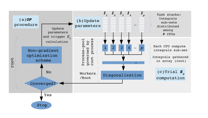
Figure 1: Process-pool solution applied for the optimization procedure ($OP$) in the context EDABI method.

IV Exemplary solution: Model of $(H_{2})_{n}$ chain

We test our solution by means of analysis performed for the chain consisting of $n=3$ hydrogen molecules stacked at intermolecular distance $a$, with the molecule bond-length $R$, and the tilt angle $\theta$. We regard this configuration as a part of periodic system (cf. Fig. 2). Hydrogen molecular chains are interesting in view of the crucial role of electronic correlations in the molecules and related low-dimension systems Kądzielawa et al. (2014); Spałek et al. (2000); Rycerz (2003). The stability of the hydrogen molecular system was studied by means of variety of methods, e.g. DFT Martínez et al. (2007) or Self-Consistent Field (SCF) Kochanski et al. (1973); Kochanski (1975), also in the context of the existence of superfluidity Mezzacapo and Boninsegni (2006).

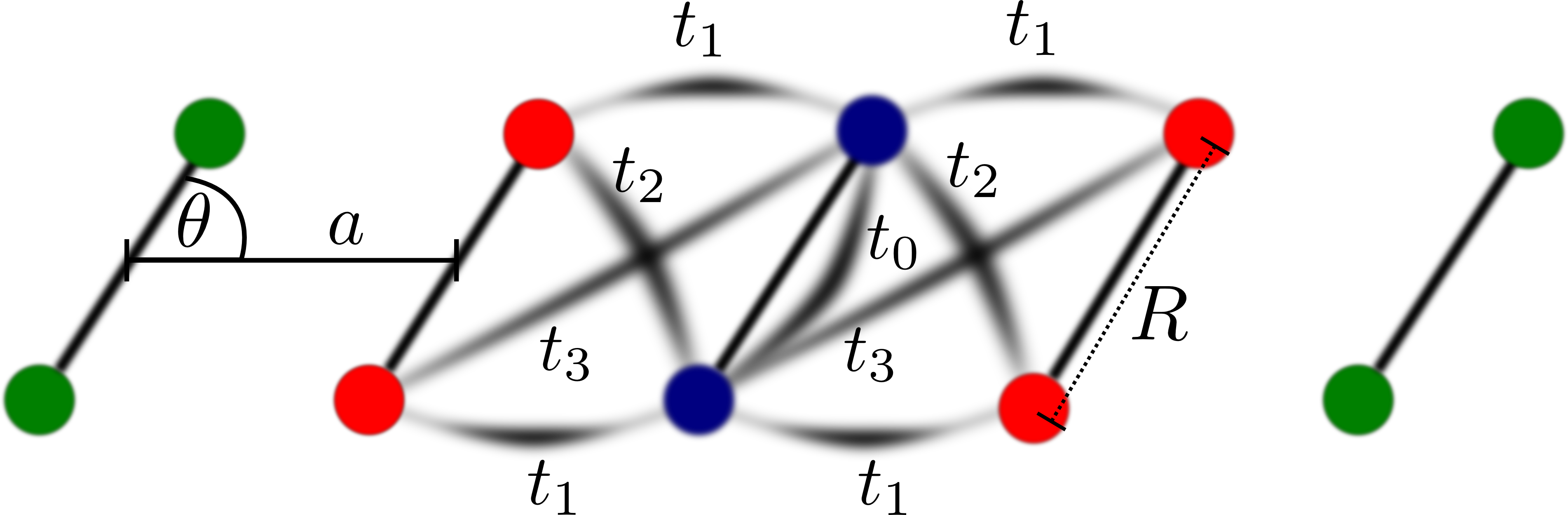
Figure 2: $(H_{2})_{n}$ molecular chain, its parametrization with possible hoppings from/to central (blue) molecule. Green molecules are included as the background field related to the system by the periodic boundary conditions.

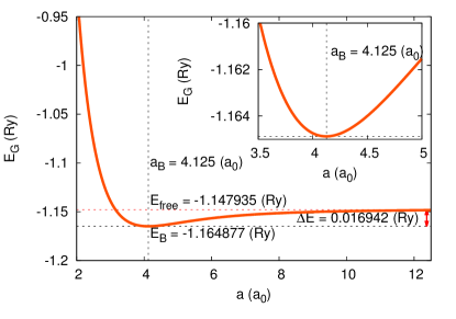
Figure 3: Ground state energy (per atom) for $(H_{2})_{3}$ molecular chain as a function of the intermolecular distance $a$. Note the convergence to analytical solution Kądzielawa et al. (2014) for the separate free molecule limit when $a\rightarrow\infty$.

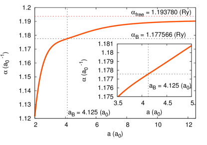
Figure 4: Inverse atomic orbital size $\alpha$ versus the intermolecular distance $a$. Note the convergence to the analytical solution Kądzielawa et al. (2014) for the separate free molecule limit when $a\rightarrow\infty$.

We discuss the molecular hydrogen chain within the so-called extended Hubbard model. This means that the interactions associated with the different atomic centers ($K_{ij}$) are taken into account. Eventually, the electronic part of Hamiltonian, with the ion-ion interaction explicitly included, can be rewritten then as composed of the three parts:

$$\mathcal{H}_{Hubb}=\sum\limits_{i}\epsilon_{i}\hat{n}_{{i}}+\sum\limits_{ij\sigma}t_{ij}c_{i\sigma}^{\dagger}c_{j\sigma}+U\sum\limits_{i}\hat{n}_{{i}\uparrow}\hat{n}_{{i}\downarrow},$$ (21a)

$$\mathcal{H}_{ext}=\mathcal{H}_{Hubb}+\frac{1}{2}\sum\limits_{ij}K_{ij}\hat{n}_{{i}}\hat{n}_{{j}},$$ (21b)

$$\mathcal{H}_{tot}=\mathcal{H}_{ext}+\frac{1}{2}\sum\limits_{ij}\frac{2}{|\mathbf{R_{i}}-\mathbf{R_{j}}|}=\mathcal{H}_{ext}+\mathcal{V}_{i-i},$$ (21c)

where the first two terms in (21a) represent the single-particle energy with all possible hoppings $t_{ij}$ (to the fourth nearest neighbor, see Fig. 2) and are calculated with respect to the background field (see Sec. IV.1 for details), $U$ is on-site Coulomb repulsion (Hubbard term), $K_{ij}$ are intersite Coulomb repulsive interactions between supercell and the background sites (see Rycerz (2003) and Appendix B for details), $\mathcal{V}_{i-i}$ is the proton–proton repulsive interaction. Despite its relative simplicity, the system exhibits non–trivial properties. However, as we focus mainly on the computational aspects, we present here only the basic physical properties. Computational performance tests of our solution are undertaken for arbitrarily chosen molecular bond–length $R=1.43042(a_{0})$, corresponding to the equilibrium value obtained by us previously for a single $H_{2}$ molecule Kądzielawa et al. (2014); also $\theta={\pi}/{2}$. The total number of electrons is equal to the number of atomic centres ($6$ for $n=3$). We test $E_{G}$ against the varying intermolecular distance $a$ (as shown in Fig. 3) obtaining the van der Waals-like behavior of the total energy, as expected Spałek et al. (2000); Rycerz (2003); Kochanski et al. (1973); Kochanski (1975). The single (spatially separated) $H_{2}$-molecule ground-state energy is reproduced asymptotically for $a\rightarrow\infty$, as marked in Fig. 3. For the sake of completeness, we present in Fig. 4 the inverse atomic orbital size $\alpha$. In Fig. 5 we plot the contours of the electronic density $n(\mathbf{r})$ as the cross–section on the $X-Y$ plane close to the configuration related to the minimal value of $E_{G}$. A very important feature of this solution worth mentioning is that as $a$ diminishes and approaches $R$ we observe a discontinuous phase transition from the molecular to the atomic states, but this feature of the results are discussed elsewhere Kądzielawa et al. (2015). Also, the minimum energy provides a stable configuration against the dissociation into separate molecules (cf. Fig. 3).

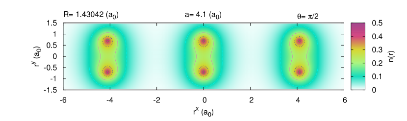
Figure 5: Electronic density $n(\mathbf{r})$ projected on $X-Y$ plane of the aligned $H_{2}$ molecules for the intermolecular distance close to the equilibrium value (marked by the vertical dashed line in Fig. 3). The values of the structure parameters are specified.

IV.1 Convergence study

We have performed the convergence study to obtain parameters suitable for the speed–up analysis of the implemented approach. There are two most important components playing crucial role: number of Gaussian functions $N_{G}$ taken in contraction (18) and the size of periodic background–field of the super-cell. The former does not require additional comment; it is not the case for the latter. With the periodic boundary conditions being imposed, a proper cut–off distance for the interactions must be also established. The atomic energy $\epsilon_{0}$ becomes in general lower when a larger number of ionic centers are taken into account (i.e., the larger cut–off distance), then the contribution from the electron–ion becomes stronger. On the other hand, analogical in nature but opposite in sign effects originate from the Coulomb ion–ion and the electron–electron repulsions. In the limit $r_{cutoff}\to\infty$ both contributions cancel each other, as discussed in the context of EDABI in Kurzyk (2007) and, for the sake of completeness, in Appendix B. One may note that the just described behavior is similar to the cancellation effect observed in the jellium model Giuliani and Vignale (2005). We define $M$ as cut–off parameter, describing the size of background field as:

$$M=\frac{r_{cutoff}}{a}$$ (22)

In Fig. 6 we plot the system total energy as a function of intermolecular distance, close to the energy-minimum configuration. It is clear that if smaller cut–off distance is selected, the energy is underestimated. If cut–off was chosen to be $\geq 150a$, the consecutive energies differ by less than the assumed numerical error in Lanczos matrix diagonalization procedure (i.e. $10^{-4}Ry\sim 1meV$). Therefore, further calculations were carried out for $M=250$, what results in $510$ integrals to be calculated after reductions caused by the system symmetries. As it follows from Fig. 7, $N_{G}=9$ is the number of Gaussians, when the energy becomes convergent, therefore the subsequent analysis corresponds to $N_{G}=9$ and $M=250$.

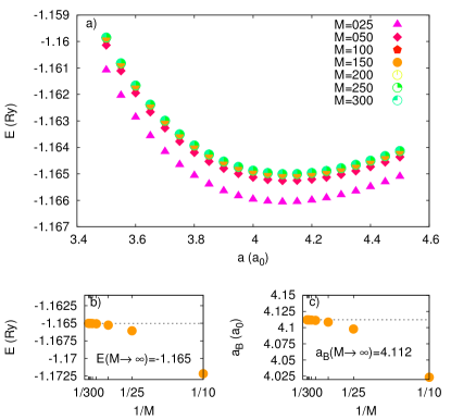
Figure 6: Convergence study: a) ground-state energy $E_{G}$ versus intermolecular parameter $a$ close to the minimum for the different background field size $M$; b) limit of $E_{G}$ for $M\rightarrow\infty$; c) limit of the optimal intermolecular parameter $a_{B}$ (minimizing $E_{G}$) for $M\rightarrow\infty$. The plots in b) and c) represent the finite-size scaling analysis.

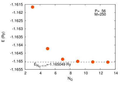
Figure 7: Convergence study: Ground-state energy $E_{G}$ versus number of Gaussians $N_{G}$ taken to represent the atomic basis and for the background field size $M=250$ and the number of SMP nodes $P=56$.

IV.2 Strong scaling for MPI+openMP solution

Taking into account that we have one electron per atomic center in a two band system (molecule consists of two hydrogen atoms), construction of the basis for three molecules leads to $924$ basis states. The diagonalization in terms of the iterative algorithm – in this case Lanczos – is not a challenge, especially if only the lowest eigenvalue is desired. A remark is necessary here: system described by substantially larger Hamiltonian matrices can also be treated efficiently in the framework of the elaborated scheme. However, more sophisticated approaches (cf. Sec. III.1) or approximate methods are then indispensable. Therefore, the example we provide, fulfills the requirement concerning the ratio of diagonalization to integration time. The latter is supposed to be the bottleneck during the execution of the optimization procedure. We investigate the speed-up ($SU$) defined as

$$SU(P,X,Y)=\frac{T_{Y}(P=1)}{T_{X}(P)},$$ (23)

with $T$ denotes time spent on the computation and

$$X,Y\in\{I,II,\varnothing\},$$ (24)

where first two symbols correspond to parallelism based on the application of openMP and openMP+MPI respectively and $\varnothing$ is associated with sequential solution. The calculations were performed for the energy optimization at given ion configuration, close to the energy minimum, allowing to collect CPU time consumed by $OP$. The measurement were covered on HP server consisting of $96$ computational nodes each supplied with the two 8–cored Intel Xeon e5-2670 2.60GHz processors. The main board supported SMP exposing one logical 16–core processor per node thus $P$ refers to the number of SMP nodes. Physically, the communication among nodes was provided by the InfiniBand 4X QDR interface. The $SU(P,II,I)$ (Fig. 8) exhibits Amdahl law–like behaviour Amdahl (1967). This law states that speed–up limit in the strong–scaling regime can be described in terms of the following formula

$$SU(P)=\frac{1}{1-f+\frac{f}{P}},$$ (25)

where $f$ is the part of the program susceptible for the parallelization. The value of $f$ was found by means of fit the Amdahl’s law to the obtained data. Approximate value of $f$ comes directly from the fit (see Fig. 8 for details) and maximal $SU$ can also be estimated by

$$SU_{max}\approx\lim_{P\to\infty}SU(P).$$ (26)

We found $f\approx 0.97$ and $SU_{max}\approx 33$, which confirms suitability of the application of our scheme. However, for the sake of completeness, we investigated the Gaussian number threshold associated with the process–pool solution efficiency.

IV.3 Number of Gaussians and Efficiency Threshold

As mentioned above, the efficiency of the process-pool solution depends on the workload assigned to each of the process in the pool. Notably, $N_{G}$ and the total number of integrals (associated with $M$ (22)) are the most important factors, influencing robustness of the proposed approach.

We have performed measurements of computation time as a function of $N_{G}$ for a different number of $P$ (see Fig. 10). For large number of Gaussians the optimization time has a universal scaling $T\sim N_{G}^{p}$, with $p\approx 4$, meaning that the two-particle integrals (20) are the most computationally expensive, as expected.

Following Schneider and Kirkpatrick (2006) we introduce the extended-Amdahl law to include potential communication overhead. In our case, the potentially most time-consuming (among $MPI$ communication routines used) $MPI\_Gather$ routine scales lineraly with $P$. Taking this into account the speed–up can be approximated by the following formula

$$SU_{comm}(P,Y,X) =\frac{1}{1-f-\delta+\frac{f}{P}+\delta P},$$ (27)

where $\delta$ is constant to be determined. We performed fit of (27) to the speed–up as a function of $P$ for $N_{G}\in\{3,5,7\}$ as we show in Fig. 9. As expected $f$ decreases with decreasing $N_{G}$, but $\delta<10^{-4}$ even for $N_{G}=3$. This value is negligible for the reasonable $P$ (the number of integrals is the upper bound) for any $f$. The lack of the communication overhead originates not only from the utilization of InfiniBand interface and linear scaling of the communication routine, but also from the small amount of data sent by each process to the root (e.g. $\sim 80$B for $P=50$). Hence the deviation from linearity for higher values of $P$ (see Fig. 10) comes from breaking the principal assumption:

For the lower numbers of Gaussians, the time of diagonalization (performed sequentially) becomes comparable or greater to that consumed by the integrals computations.

The analysis performed above allows to describe the boundaries where the proposed solution is effective. However, from the users perspective the most compelling feature is the absolute speed-up $SU(P,II,\varnothing)$, as it is the metric for the time save. In the next paragraph we present this result.

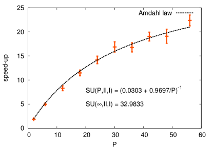
Figure 8: Speed-up ($SU$) as a function of number of processes $P$. Amdahl law curve fited to data. Each point probed 50 times.

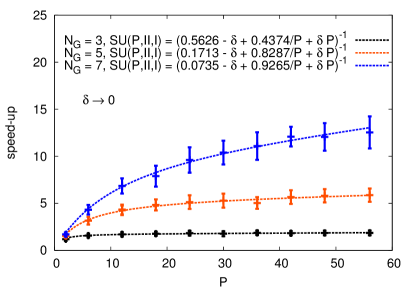
Figure 9: The relative speed-up $SU$ (23) versus number of nodes $P$ for $N_{G}\in\{3,5,7\}$ measured $100$ times. Note that when fitting the so-called extended Amdahl law, communication overhead factor $\delta\approx 0$. Note that for $N_{G}=3$ only $44\%$ of the program is performed parallelly.

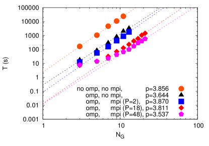
Figure 10: Computation time as a function of $N_{G}$ for sequential, only openMP, and MPI+openMP solutions. Note the linear behavior in the regime of large $N_{G}$ on log–log scale, suggesting $T\sim N_{G}^{p}$. Values found from fit (see key) are consistent with ideal case $p=4$, where whole time is spent on calculating two-body integrals (20). As one-body integrals have $p=2$, values tend to drift from $4$.

IV.4 Absolute Speed-up

Whilst analysis of the speed–up in strong scaling regime allowed us to investigate the efficiency gain in terms of a number of processes engaged in computation it is interesting and important to answer what is the absolute acceleration $SU(P,II,\varnothing)$. Obviously, this quantity still depends on $P$. In Tab. 1 we show the values of the speed-up (23) for different number of nodes $P$. The extremal case ($P=56$ with both levels of parallelization) the speed-up

$$SU\left(56,II,\varnothing\right)=303.418.$$ (28)

However, even for the lower number of SMP nodes ($P$) the absolute speed–up is excellent. For the sake of completeness, we retrieved the acceleration associated with openMP utilization (fourth column in Tab. 1). As each SMP node consisted of 16 cores the number of active threads was the same. We obtained $SU(P,II,I)$ by means of the identity

$$SU\left(P,II,I\right)=\frac{SU\left(P,II,\varnothing\right)}{SU\left(P,I,\varnothing\right)}.$$ (29)

We found good speed–up ratio $\sim 13$ (while the upper bound is $16$) coming from collapsing of nested loops (20).

Table 1: Values of the speed-up (SU) for one– and two-level parallelism for the different number of nodes $\mathbf{P}$.

P	SU(P,I,$\varnothing$)	SU(P,II,$\varnothing$)	SU(P,II,I)
2	$1.866$	$25.304$	$13.561$
6	$4.969$	$67.382$	$13.561$
12	$8.288$	$112.391$	$13.561$
18	$11.479$	$155.656$	$13.561$
24	$14.174$	$192.207$	$13.561$
30	$16.870$	$228.763$	$13.561$
36	$16.779$	$227.531$	$13.561$
42	$19.026$	$258.007$	$13.561$
48	$19.085$	$258.811$	$13.561$
56	$22.375$	$303.418$	$13.561$

V Conclusions

We have presented an effective computational approach related to the EDABI method - quantum–mechanical approach allowing to treat the electronic correlations in a consistent manner. This means that we combine the second-quantization aspect (evaluation of energies for different many-particle configurations) with an explicit evaluation of the renormalized wave functions (first-quantization aspect) in the resultant correlated many-particle state. The number of microscopic parameters that are necessary for description of the physical system can be meaningful in many cases. Hence, their computations become challenging as an effect of numerical complexity caused by the vast number of integrations to be performed (9). Here we have addressed in detail the part of the whole problem that is associated with the single-particle basis optimization. We have proposed the scheme based on the process–pool concept enhanced by the two–level parallelism, and test it utilizing self–made generic implementation Biborski and Kądzielawa (2014) configured for the specific computational problem – $\left(H_{2}\right)_{n}$ chain. The proposed approach is intuitive and has allowed us to speed up the calculations significantly (of the order of $10^{2}$) while preserving its generic character. Employing process–pool solution to other systems is then straightforward.

Since the considered physical example serves as an illustration of the elaborated scheme capability, one may consider engaging it to a wide class of computationally advanced physical problems tractable within the framework of EDABI or similar methods. Such problems cover:

• lattice vibration (phonon) spectrum via the so-called direct method (where all but few symmetries are lost, increasing the number of integrals dramatically – from $510$ to over $10\ 000$ for $\left(H_{2}\right)_{n}$ chain);

• calculation of the electron–lattice coupling parameters in direct space;

• electronic structure calculations of the realistic two– and three-dimensional atomic and molecular crystals (e.g. hydrogen, lithium hydride), where both the number of atomic orbitals and the background field increase essentially.

Neither form of the starting Hamiltonian nor the diagonalization scheme choice is essential for the applicability of the method, allowing us to incorporate other approaches such as the Gutzwiller approximation Wysokiński et al. (2014, 2015); Kądzielawa et al. (2013) or Gutzwiller Wave Function - Diagramatic Expansion Kaczmarczyk et al. (2014) to study molecular and extended spatially systems. In this manner, one can address e.g. the fundamental question of metallization in correlated systems Gebhard (1997); Koch et al. (2000) with the explicit evaluation of an model parameters. So far we have been able to solve exactly the chain with $N=3$, $4$, $5$, and $6$ molecules and the results are of similar type Kądzielawa et al. (2015). The finite-size type of scaling on the basis of these results requires additional analysis.

VI Acknowledgments

The authors are grateful to the Foundation for Polish Science (FNP) for financial support within the Project TEAM and to the National Science Center (NCN) for the support within the Grant MAESTRO, No. DEC-2012/04/A/ST3/00342. We are also grateful to dr hab. Adam Rycerz from the Jagiellonian University for helpful comments.

Appendix A EDABI method: A brief overview

The Exact Diagonalization Ab Initio (EDABI) approach combines first- and second-quantization aspects when solving the many-particle problem as expressed formally by its Hamiltonian.

The starting Hamiltonian (8) contains all possible dynamical processes starting from two-body interaction $V(r-r^{\prime})$ in the coordinate (Schrödinger) representation. Its version (10) is already truncated and limited to two-state (here two-site) terms, i.e., the three- and four-site terms have been neglected. The rationale behind this omission is that, as shown elsewhere Spałek et al. (2000, 2007), already the two-site terms (matrix elements) $\sim J_{ij}$ and $V_{ij}$ are much smaller than those $\sim U$ and $K_{ij}$. Parenthetically, all the terms are taken into account in the starting atomic basis composing the Wannier function. Nonetheless, there is no principal obstacle in including all those terms in the case of the small systems considered here.

The second characteristic feature of EDABI is the single-particle basis optimization which composes the main topic of this paper. If the basis defining the starting Wannier-function basis were complete (i.e., $L\rightarrow\infty$ in Eq. (13)), then no basis optimization is required and an exact solution is achieved. However, as our basis $\{w_{i}\}$ is incomplete one, in our view, we are forced to readjust the basis so that the system dynamics (correlations) are properly accounted for. This introduces a variational aspect to our solution, since we introduce a variable wave function size, adjustable in the interacting (correlated) state. This very feature represents one of the factors defining the method. Such adjustment is also reasonable from a physical point of view, as the single-particle orbital adapts then itself to the presence of other particles (electrons). In other words, the correlations induced by the predominant interaction terms ($\sim U$ and $K_{ij}$) influence the size and shape of the states $\{w_{i}(\mathbf{r})\}$. This means that the orbitals get renormalized in the process of the correlated state formation. Nonetheless, it is not a priori determined that negligence of the higher virtually excited states in the expansion (13) is minimized is such a manner. This should be tested and is one of the subjects of our current research. This is not the primary topic of this paper so we shall not dwell upon it any further here.

Note also that by selecting the diagonalization of many-particle Hamiltonian in the second-quantized form, one avoids writing the many-determinantal expansion of the multiparticle wave function, as is the case in the CI methods. However, out of our formulation one can obtain the function $\Psi(\mathbf{r}_{1},\dots,\mathbf{r}_{N})$ and in particular, define many-particle covalency Spałek et al. (2007). This transition from the Fock space back to the Hilbert space is possible as the two languages of description are equivalent in the nonrelativistic situation (for a lucid and didactic exposition of the first- and second-quantization schemes and their equivalence see e.g. Robertson (1973)). The principal limitation of our method is the circumstance that it can be applied directly only to relatively small systems when the exact diagonalization is utilized.

Appendix B Convergence of the single-particle energy for infinite system

In (21a) we have the microscopic parameter contained in the single-particle energy expression, namely

$$\epsilon_{i}=\left\langle\psi_{i}\vphantom{\left(-\bigtriangledown^{2}-\sum_{j}\frac{2}{\left|\mathbf{r}-\mathbf{R}_{j}\right|}\right)\psi_{i}}\right|\left(-\bigtriangledown^{2}-\sum_{j}\frac{2}{\left|\mathbf{r}-\mathbf{R}_{j}\right|}\right)\left|\psi_{i}\vphantom{\psi_{i}\left(-\bigtriangledown^{2}-\sum_{j}\frac{2}{\left|\mathbf{r}-\mathbf{R}_{j}\right|}\right)}\right\rangle,$$ (30)

where $i$ labels lattice site (node) at which we calculate this single-particle energy, and $j$ goes over the whole system. Also, $\psi_{i}$ is the $1s$ Slater-type orbital centered on that site. For the sake of clarity, we disregard the orthogonalization procedure, as the one-body parameters contain, strictly speaking, a linear combination of integrals in STO basis.

For an infinite system, the sum $\sum_{j}$ constitutes a series of the form Slater (1963)

$$\epsilon_{i}= -\left\langle\psi_{i}\vphantom{\bigtriangledown^{2}\psi_{i}}\right|\bigtriangledown^{2}\left|\psi_{i}\vphantom{\psi_{i}\bigtriangledown^{2}}\right\rangle-\sum_{j}\left\langle\psi_{i}\vphantom{\frac{2}{\left|\mathbf{r}-\mathbf{R}_{j}\right|}\psi_{i}}\right|\frac{2}{\left|\mathbf{r}-\mathbf{R}_{j}\right|}\left|\psi_{i}\vphantom{\psi_{i}\frac{2}{\left|\mathbf{r}-\mathbf{R}_{j}\right|}}\right\rangle$$ (31)

$$= \alpha^{2}-2\alpha-\sum_{j}\frac{2}{\left|\mathbf{R}_{ij}\right|}+2\left(\alpha+\frac{1}{\left|\mathbf{R}_{ij}\right|}\right)e^{-2\alpha\left|\mathbf{R}_{ij}\right|},$$

which diverges to $-\infty$. In this Appendix we show that there is an effective single-particle energy with no divergence for the infinite systems (case more general than those discussed in Rycerz (2003); Kurzyk (2007)).

We start from Hamiltonian (21c)

$$\mathcal{H}_{tot}=\mathcal{H}_{ext}+\mathcal{V}_{i-i},$$ (32)

where ion–ion interaction is defined in the classical limit, i.e.,

$$\mathcal{V}_{i-i}\equiv\frac{1}{2}\sum_{i\neq j}\frac{2}{\left|\mathbf{R}_{ij}\right|},$$ (33)

and $\left|\mathbf{R}_{ij}\right|$ is the distance between sites $i$ and $j$. We analyze next the remaining contributions, term by term.

B.1 Intersite Coulomb term

The intersite Coulomb term from (21b) cab be rewritten in the form

$$\frac{1}{2}\sum\limits_{ij}K_{ij}\hat{n}_{{i}}\hat{n}_{{j}}= \stackrel{{\scriptstyle K^{(0)}}}{{\overbrace{\frac{1}{2}\sum_{i\neq j}K_{ij}\delta\hat{n}_{{i}}\delta\hat{n}_{{j}}}}}+\stackrel{{\scriptstyle K^{(1})}}{{\overbrace{\frac{1}{2}\sum_{i}\sum_{j}\left(1-\delta_{ij}\right)K_{ij}\hat{n}_{{i}}}}}$$

$$+ \stackrel{{\scriptstyle K^{(2)}}}{{\overbrace{\frac{1}{2}\sum_{i}\sum_{j}\left(1-\delta_{ij}\right)K_{ij}\hat{n}_{{j}}}}}-\stackrel{{\scriptstyle K^{(3)}}}{{\overbrace{\frac{1}{2}\sum_{i\neq j}K_{ij}}}},$$ (34)

where $\delta\hat{n}_{{i}}\equiv\left(\hat{n}_{{i}}-1\right)$ and $\delta_{ij}$ is Kronecker’s delta.

We observe that when all sites are taken into account, the terms $K^{(1)}$ and $K^{(2)}$ are equivalent. We can rewrite them as follows

$$\mathcal{H}_{\text{K}}= K^{(0)}-K^{(3)}+2\ \frac{1}{2}\sum_{i}\sum_{j}\left(1-\delta_{ij}\right)K_{ij}\hat{n}_{{i}}=$$ (35)

$$\approx K^{(0)}-K^{(3)}+2\ \frac{1}{2}\sum_{i}\hat{n}_{{i}}\sum_{j(i)}K_{ij},$$

where $j(i)$ denotes the neighborhood of site $i$. Likewise,

$$K^{(3)}= \frac{1}{2}\sum_{i\neq j}K_{ij}=\frac{1}{2}\sum_{i}\sum_{j(i)}K_{ij}.$$ (36)

We can write finally that

$$\mathcal{H}_{\text{K}}= K^{(0)}+\frac{1}{2}\sum_{i}\hat{n}_{{i}}\sum_{j(i)}K_{ij}$$ (37)

$$+ \frac{1}{2}\sum_{i}\delta\hat{n}_{{i}}\sum_{j(i)}K_{{i}j}.$$

Note that for half-filling $\left\langle\hat{n}_{{i}}\right\rangle=1$ and the last part and $\left\langle K^{(0)}\right\rangle$ disappears.

B.2 Ion-ion repulsion

Similarly, we can rewrite (33) to the form

$$\mathcal{V}_{i-i}= \frac{1}{2}\sum_{i\neq j}\frac{2}{\left|\mathbf{R}_{ij}\right|}\approx\frac{1}{2}\sum_{i}\sum_{j(i)}\frac{2}{\left|\mathbf{R}_{ij}\right|}=\frac{1}{2}N\sum_{j({i_{0}})}\frac{2}{\left|\mathbf{R}_{{i_{0}}j}\right|}$$

$$= \frac{1}{2}\sum_{i}\hat{n}_{{i}}\sum_{j({i})}\frac{2}{\left|\mathbf{R}_{{i}j}\right|}-\frac{1}{2}\sum_{i}\delta\hat{n}_{{i}}\sum_{j({i})}\frac{2}{\left|\mathbf{R}_{{i}j}\right|}.$$ (38)

Again, the average of the latter term disappears for one particle per site.

B.3 Total Hamiltonian

We rearrange (21c) obtaining so that the new form of Hamiltonian is

$$\mathcal{H_{N}}=\mathcal{H}_{\epsilon^{\text{eff}}}+\mathcal{H}_{\text{Hubbard}}+\mathcal{H}_{\delta n}.$$ (39)

The new terms are

$$\mathcal{H}_{\epsilon^{\text{eff}}}=\sum_{i}\epsilon^{\text{eff}}_{i}\hat{n}_{{i}},$$ (40)

with $\epsilon^{\text{eff}}_{i}=\epsilon_{i}+1/2\sum_{j({i})}\left({2}/{\left|\mathbf{R}_{{i}j}\right|}+K_{{i}j}\right)$,

$$\mathcal{H}_{\text{Hubbard}}= \sum\limits_{ij}\sum\limits_{\sigma}t_{ij}c_{i\sigma}^{\dagger}c_{j\sigma}+U\sum\limits_{i}\hat{n}_{{i}\uparrow}\hat{n}_{{i}\downarrow},$$ (41)

$$\mathcal{H}_{\delta n}= \frac{1}{2}\sum_{i\neq j}K_{ij}\delta\hat{n}_{{i}}\delta\hat{n}_{{j}}+$$ (42)

$$+\frac{1}{2}\sum_{i}\delta\hat{n}_{{i}}\sum_{j(i)}\left(K_{{i}j}-\frac{2}{\left|\mathbf{R}_{{i}j}\right|}\right).$$

The last question is whether the effective single-particle energy is now convergent.

B.4 Convergence of the single-particle energy

We can take $\epsilon^{\text{eff}}_{i}$ from eqs. 40 and 31 and rearrange it in a following manner

$$\epsilon^{\text{eff}}_{i}= \epsilon_{i}+\frac{1}{2}\sum_{j}\left(\frac{2}{\left|\mathbf{R}_{ij}\right|}+K_{ij}\right)$$ (43)

$$= \alpha^{2}-2\alpha+\sum_{j}-\frac{2}{\left|\mathbf{R}_{ij}\right|}+2\left(\alpha+\frac{1}{\left|\mathbf{R}_{ij}\right|}\right)e^{-2\alpha\left|\mathbf{R}_{ij}\right|}$$

$$+\frac{1}{2}\sum_{j}\left(\frac{2}{\left|\mathbf{R}_{ij}\right|}+K_{ij}\right)$$

$$= \alpha^{2}-2\alpha+\sum_{j}2\left(\alpha+\frac{1}{\left|\mathbf{R}_{ij}\right|}\right)e^{-2\alpha\left|\mathbf{R}_{ij}\right|}$$

$$+\sum_{j}\left(\frac{1}{\left|\mathbf{R}_{ij}\right|}+\frac{1}{2}K_{ij}-\frac{2}{\left|\mathbf{R}_{ij}\right|}\right).$$

The latter part disappears in the classical limit $\left|\mathbf{R}_{ij}\right|\gg\alpha^{-1}$, where

$$K_{ij}\rightarrow\frac{2}{\left|\mathbf{R}_{ij}\right|},$$ (44)

and the remaining part $\sum_{j}2\left(\alpha+{\left|\mathbf{R}_{ij}\right|^{-1}}\right)e^{-2\alpha\left|\mathbf{R}_{ij}\right|}$ is convergent.

References

- Himmetoglu et al. (2014) B. Himmetoglu, A. Floris, S. de Gironcoli, and M. Cococcioni, Int. J. Quant. Chem. 114, 14 (2014).
- Karolak et al. (2010) M. Karolak, G. Ulm, T. Wehling, V. Mazurenko, A. Poteryaev, and A. Lichtenstein, J. Electron. Spectrosc. Relat. Phenom. 181, 11 (2010).
- Spałek et al. (2000) J. Spałek, R. Podsiadły, W. Wójcik, and A. Rycerz, Phys. Rev. B 61, 15676 (2000).
- Spałek et al. (2007) J. Spałek, E. Görlich, A. Rycerz, and R. Zahorbeński, J. Phys.: Condens. Matter 19, 255212 (2007), pp. 1-43.
- Surjan (1989) P. Surjan, Second Quantizied Approach to Quantum Chemistry (Springer, Berlin, 1989).
- Kądzielawa et al. (2014) A. P. Kądzielawa, A. Bielas, M. Acquarone, A. Biborski, M. M. Maśka, and J. Spałek, New J. Phys. 16, 123022 (2014).
- Rycerz (2003) A. Rycerz, Physical properties and quantum phase transitions in strongly correlated electron systems from a combined exact diagonalization – ab initio approach, Ph.D. thesis, Jagiellonian University (2003).
- Kądzielawa et al. (2013) A. P. Kądzielawa, J. Spałek, J. Kurzyk, and W. Wójcik, Eur. Phys. J. B 86, 252 (2013).
- Hubbard (1963) J. Hubbard, Proc. Roy. Soc. (London) 276, 238 (1963).
- Gutzwiller (1963) M. C. Gutzwiller, Phys. Rev. Lett. 10, 159 (1963).
- Gutzwiller (1965) M. C. Gutzwiller, Phys. Rev. 137, A1726 (1965).
- Kanamori (1963) J. Kanamori, Prog. Theor. Phys. 30, 275 (1963).
- Zegrodnik and Spałek (2012) M. Zegrodnik and J. Spałek, Phys. Rev. B 86, 014505 (2012).
- Zegrodnik et al. (2014) M. Zegrodnik, J. Bünemann, and J. Spałek, New J. Phys. 16, 033001 (2014).
- Wysokiński et al. (2014) M. M. Wysokiński, M. Abram, and J. Spałek, Phys. Rev. B 90, 081114(R) (2014).
- Siro and Harju (2012) T. Siro and A. Harju, Comput. Phys. Commun. 183, 1884 (2012).
- Wendt et al. (2011) K. A. Wendt, J. E. Drut, and T. A. Lähde, Comput. Phys. Commun. 182, 1651 (2011).
- Dirac (1927) P. A. M. Dirac, Proc. Roy. Soc. (London) A 114, 243 (1927).
- Fock (1932) V. Fock, Z. Phys. 75, 622 (1932).
- Fetter and Walecka (2003) A. L. Fetter and J. D. Walecka, Quantum Theory of Many-Particle Systems (Dover, 2003).
- Wysokiński et al. (2015) M. M. Wysokiński, M. Abram, and J. Spałek, Phys. Rev. B 91, 081108 (2015).
- Ashcroft and Mermin (1976) N. Ashcroft and N. Mermin, Solid State Physics (Saunders College, Philadelphia, 1976).
- Mulliken (1935) R. S. Mulliken, J. Chem. Phys. 3, 375 (1935).
- Kurzyk et al. (2008) J. Kurzyk, W. Wójcik, and J. Spałek, Eur. Phys. J. B 66, 385 (2008).
- Martínez et al. (2007) J. I. Martínez, M. Isla, and J. A. Alonso, Eur. Phys. J. D 43, 61 (2007).
- Kochanski et al. (1973) E. Kochanski, B. Roos, P. Siegbahn, and M. Wood, Theoret. Chim. Acta (Berl.) 32, 151 (1973).
- Kochanski (1975) E. Kochanski, Theoret. Chim. Acta (Berl.) 39, 339 (1975).
- Mezzacapo and Boninsegni (2006) F. Mezzacapo and M. Boninsegni, Phys. Rev. Lett. 97, 045301 (2006).
- Kądzielawa et al. (2015) A. P. Kądzielawa, A. Biborski, and J. Spałek, arXiv: 1506.3356 (2015).
- Kurzyk (2007) J. Kurzyk, Układy skorelowanych elektronów o różnej wymiarowości z uwzględnieniem optymalizacji jednocząstkowej funkcji falowej, Ph.D. thesis, Jagiellonian University (2007), in Polish.
- Giuliani and Vignale (2005) G. F. Giuliani and G. Vignale, Quantum Theory of the Electron Liquid (Cambridge, 2005).
- Amdahl (1967) G. M. Amdahl, in Proceedings of the April 18-20, 1967, Spring Joint Computer Conference, AFIPS ’67 (Spring) (ACM, New York, 1967) pp. 483–485.
- Schneider and Kirkpatrick (2006) J. Schneider and S. Kirkpatrick, Stochastic Optimization (Springer, Berlin, 2006).
- Biborski and Kądzielawa (2014) A. Biborski and A. Kądzielawa, “QMT: Quantum Metallization Tools Library,” (2014).
- Kaczmarczyk et al. (2014) J. Kaczmarczyk, J. Bünemann, and J. Spałek, New J. Phys. 16, 073018 (2014).
- Gebhard (1997) F. Gebhard, The Mott Metal-Insulator Transition: Models and Methods (Springer, Berlin, 1997).
- Koch et al. (2000) E. Koch, O. Gunnarsson, and R. M. Martin, Comput. Phys. Commun. 127, 137 (2000).
- Robertson (1973) B. Robertson, Am. J. Phys. 41, 678 (1973).
- Slater (1963) J. C. Slater, Quantum Theory of Molecules and Solids, Vol. 1 (McGraw-Hill, New York, 1963).