Influence Maximization under The Non-progressive Linear Threshold Model

Abstract

In the problem of influence maximization in information networks, the objective is to choose a set of initially active nodes subject to some budget constraints such that the expected number of active nodes over time is maximized.

The linear threshold model has been introduced to study the opinion cascading behavior, for instance, the spread of products and innovations. In the existing studies, the study of the linear threshold model mainly focus on the progressive case, in which once a user became active, it is forced to be active forever. In this paper, we consider the non-progressive case in which active nodes might become inactive in subsequent time steps. This setting makes it possible to model the users’ dynamic behavior, and consequently fit better to the situation of continuous consumption in the daily life. Previous works on the non-progressive case assumed that the thresholds indicating the susceptibilities of the individuals change randomly and independently at every time step. We argue that an individual’s susceptibility should be consistent, and hence it is more realistic to consider the case in which an individual’s susceptibility is chosen initially at random, but then remains the same throughout the process. This setting causes more completeness for the analysis, as for any two nodes that share a common ancestor, their status are no longer independent.

In this paper, we we extends the classic linear threshold model [18] to capture the non-progressive behavior. The information maximization problem under our model is proved to be NP-Hard, even for the case when the underlying network has no directed cycles. The first result of this paper is negative. In general, the objective function of the extended linear threshold model is no longer submodular, and hence the hill climbing approach that is commonly used in the existing studies is not applicable. Next, as the main result of this paper, we prove that if the underlying information network is directed acyclic, the objective function is submodular (and monotone). Therefore, in directed acyclic networks with a specified budget we can achieve $\frac{1}{2}$-approximation on maximizing the number of active nodes over a certain period of time by a deterministic algorithm, and achieve the $(1-\frac{1}{e})$-approximation by a randomized algorithm.

1 Introduction

We consider the problem of an advertiser promoting a product in a social network. The idea of viral marketing [8, 17] is that with a limited budget, the advertiser can persuade only a subset of individuals to use the new product, perhaps by giving out a limited number of free samples. Then the popularity of the product is spread by word-of-mouth, i.e. through the existing connections between users in the underlying social network.

Information networks have been used to model such cascading behavior  [23, 8, 9, 13, 14, 18, 19]. An information network is a directed edge-weighted graph, in which a node represents a user, whose behavior is influenced by its (outgoing) neighbors, and the weight of an edge reflects how influential the corresponding neighbor is. A node adopting the new behavior is active and is otherwise inactive. The threshold model [15, 18] is one way to model the spread of the new behavior. The resistance of a node $v$ to adopt the new behavior is represented by a random threshold $\theta_{v}$ (higher value means higher resistance), where the randomness is used to model the different susceptibility of different users. The new behavior is spread in the information network in discrete time steps. An inactive node changes its state to active if the weighted influence from the active neighbors in the previous time step reaches its threshold. We consider the non-progressive case where an active node could revert back to the inactive state if the influence from its neighbors drops below its threshold.

Our Contribution.

We consider the non-progressive linear threshold model in this paper, which is the natural extension of the well known linear threshold model [18]. In Section 2, the formal definition of the non-progressive linear threshold model is introduced, as well as the influence maximization problem. In most existing works, for a set of initially active nodes, the influence is measured by the maximum number of active nodes. Since the existing works consider the progressive case, hence the number of active nodes increases step by step and achieves the maximum after at most $n$ time steps, where $n$ is the number of the nodes. However, in the non-progressive case, it is possible that the active status never become stable. Hence, we introduce the average number of active nodes over a time period to measure the influence. Similar to the progressive case, the influence maximization problem considering the non-progressive linear threshold model is also NP-hard (Section 3). In order to approximate the optimal within a constant factor, a commonly used approach is to prove the monotone and submodular property of the objective function. Then the constant approximation ratio algorithms are promised by using the results of Fisher et al. [12] and Calinescu et al. [3]. However, this approach is not generally applicable for the non-progressive linear threshold model, since as showed in Section 4, the average number of active nodes is possibly not submodular. As the main result of this paper, we studied the case when the information network is acyclic. As consistent with the intuition, the expected influence under the acyclic networks is submodular and hence Fisher’s technique (and Calinescu’s technique) is applicable to achieve the constant approximation. It should be noted that although the acyclic case looks much simpler than the general ones (where directed cycles may exist), the solution to maximize the expected influence is not that easy. As it is proved in Section 3, the problem of influence maximization is still NP-Hard even for the case under acyclic information networks. Futhermore, to prove the submodularity of the expected influence, we still need some tricky technique (in this paper, we ) to handle complicated association between the status of the nodes. To see the association, consider time $t>0$, the status of nodes at time $t$ are associated if they share some common ancestors and the threshold of such an ancestor affects the status of its descendants. As this kind of association exist, it requires more carefully consideration of the nodes status and the analysis consequently become more complicate. In Section 5, we introduce an equivalent process (called Path Effect) for the non-progressive linear threshold model, and then the deep connection between this process and the random walk is proved via a coupling technique, which consequently leads to our final conclusion of the submodularity of the expected influence (under non-progressive linear threshold model).

Related Works.

The cascading behavior in information networks was first studied in the computer science community by Kempe, Kleinberg and Tardos [18]. They considered the Independent Cascade Model and the Linear Threshold Model, the latter of which we generalize in this paper. Their main focus was the progressive case, and only reduced the non-progressive case to the progressive one by assigning a new independent random threshold to each node at every time step such that the resulting objective function is still submodular.

Kempe et al. [18, 19] have also shown that the influence maximization problem in such models is NP-hard. Researchers often first show that the objective functions in question are submodular and then apply submodular function maximization methods to obtain constant approximation ratio. An example of such methods is the Standard Greedy Algorithm, which is analyzed by by Nemhauser and Fisher et al. [22, 12]. Loosely speaking, the Standard Greedy Algorithm (also known as the Hill Climbing Algorithm) starts with an empty solution, and in each iteration while there is still enough budget, we expand the current solution by including an additional node that causes the greatest increase in the objective function. Although the costs for transient and permanent nodes are different in our model, the budget constraint can still be described by a matroid. Under the matroid constraint, Fisher et al. [12] showed that the Standard Greedy Algorithm achieves $\frac{1}{2}$-approximation, and Calinescu et al. [3] introduced a randomized algorithm that achieves $(1-\frac{1}{e})$-approximation in expectation.

In the above submodular function maximization algorithms, the objective function needs to be accessed in each iteration. However, to calculate the exact value of the objective function is in general hard [7]. One way to resolve this is to estimate the value of the objective function by sampling. Some works have used other ways to overcome this issue. To improve the efficiency of the Standard Greedy Algorithm, Leskovec et al. [20] showed a Cost-Effective Lazy Forward scheme, which makes use of the submodularity of the objective function and avoids the evaluation of influence on those nodes for which the incremental influence in the previous iteration is less than that of some already evaluated node in the current iteration. This scheme has been shown more efficient than the Standard Greedy Algorithm by experiments. Chen et al. [6] also designed an improved scheme to speed up the Standard Greedy Algorithm by using some efficiently computable heuristics that have similar performance.

Chen et al. [5] considered how positive and negative opinions spread in the same network, which can be interpreted as the influence process involving two agents. The influence maximization problem considering multiple competing agents in an information network has also been studied in [16, 10, 2, 4]. We follow a similar setting in which a new comer can observe the strategies of existing agents, and stategizes accordingly to maximize his influence in the network.

Mossel and Roch [21] have shown that under more general submodular threshold functions (as opposed to linear threshold functions), the objective function is still submodular and hence the same maximization framework can still be applied.

Similar to our approach, the relationship between influence spreading and random walks has been investigated by Asavathiratham et al. [1], and Even-Dar and Shapira [11] in other information network models.

2 Preliminaries

      Definition 1 (Information Network).

An information network is a directed weighted graph $G=(V,E,b)$ with node set $V$ and edge set $E$, where each edge $(v,u)\in E$ has some positive weight $0<b_{vu}<1$ which intuitively represents the influencing power of $u$ on $v$. Denote the set of outgoing neighbors of a node $v$ by $\Gamma(v):=\{u\in V\mid(v,u)\in E\}$. In addition, for each $v\in V$, the total weight of its outgoing edges is at most $1$, i.e. $\sum_{u\in\Gamma(v)}b_{vu}\leq 1$.

Without loss of generality, we assume that in the considered information network $G$, $\sum_{u\in\Gamma(v)}b_{vu}$ is exactly $1$ for every node $v\in V$. To achieve this requirement, for any given $G$, we add a void node $d$ and for each node $v\neq d$, we include $(v,d)$ into the set of edges, and set $b_{vd}:=1-\sum_{u\in\Gamma(v)\setminus\{d\}}b_{vu}$. We can add a self loop with weight $1$ at the void node $d$. Furthermore, $d$ is never allowed to be active initially, and hence will never be active. Unless explicitly specified, when we use the term node in general, we mean a node other than the void node.

Next, we formally describe the extension of the classic linear threshold model for the adaption of the non-progressive behavior. A new feature of our model is that an initially active node can be either transient or permanent.

      Model 1 (Non-progressive Linear Threshold Model (NLT)).

Consider an information network $G=(V,E,b)$. Each node in $V$ is associated with a threshold $\theta_{v}$, which is chosen from $(0,1)$ independently and uniformly at random. At time $t\geq 0$, every node $v$ is either active $\mathcal{A}$ or inactive $\mathcal{N}$. Denote the set of active nodes at time $t$ by $A_{t}$. In the influence process, given a transient initial set $A\subseteq V$, a permanent initial set $\widehat{A}\subseteq V$, and a configuration of thresholds $\mathbb{\theta}=\{\theta_{v}\}_{v\in V}$, the nodes update their status according to the following rules.

• At time $t=0$, $A_{0}:=A\cup\widehat{A}$.

• At time $t>0$, for each node $v\in V\setminus\widehat{A}$, compute the activation function $f_{v}(A_{t-1}):=\sum_{u\in A_{t-1}\cap\Gamma(v)}b_{vu}$. Then let $A_{t}:=\{v\in V\setminus\widehat{A}|f_{v}(A_{t-1})\geq\theta_{v}\}\cup\widehat{A}$.

Without loss of generality, we can assume $A\cap\widehat{A}=\emptyset$, otherwise we can use $A\setminus\widehat{A}$ as the transient initial set instead. Given a transient initial set $A$ and a permanent initial set $\widehat{A}$, we measure the influence of the agent by the average number of active nodes over $T$ time steps, where $T$ is some pre-specified time scope in which the process evolves. Observe that once the initial sets and the configuration of the thresholds are given, the active sets $A_{t}$’s are totally determined.

      Definition 2 (Influence Function and Expected Influence).

Given an information network $G$, a transient initial set $A$, a permanent initial set $\widehat{A}$, and a configuration $\theta$ of thresholds, the average influence over time period $[1,T]$ is defined as $\sigma^{[1,T]}_{\theta}(A,\widehat{A}):=\frac{1}{T}{\sum^{T}_{t=1}\mid A_{t}\mid}$. For simplicity, we ignore the superscript $[1,T]$ in $\sigma$ when the target period is clear from the context. We define the expected influence $\overline{\sigma}$ as the expectation of $\sigma_{\theta}(A,\widehat{A})$ over the random choice of $\theta$, i.e., $\overline{\sigma}(A,\widehat{A}):=\mathbb{E}_{\theta}[\sigma_{\theta}(A,\widehat{A})]$.

      Definition 3 (Influence Maximization Problem).

In an information network $G$, suppose the advertising cost of a transient initial node is $c$ and that of a permanent initial node is $\widehat{c}$, where the costs are uniform over the nodes. Given a budget $K$, the goal is to find a transient initial set $A$ and a permanent initial set $\widehat{A}$ with total cost $c\cdot|A|+\widehat{c}\cdot|\widehat{A}|$ at most $K$ such that $\overline{\sigma}(A,\widehat{A})$ is maximized.

The most technical part of the paper is to show that the objective function $\overline{\sigma}$ is submodular so that the maximization techniques of Fisher et al. [12] can be applied.

      Definition 4 (Submodular, Monotone).

A function $f:2^{V}\rightarrow\mathbb{R}$ is submodular if for any $A\subseteq B\subseteq V$ and $w\in V\setminus B$, $f(B\cup\{w\})-f(B)\leq f(A\cup\{w\})-f(A)$ holds. A function $f$ is monotone if for any $A\subseteq B$, $f(A)\leq f(B)$. A function $g:2^{V}\times 2^{V}\rightarrow\mathbb{R}$ is submodular (monotone), if keeping one argument constant, the function is submodular (monotone) as a function on the other argument.

In order to facilitate the analysis of the influence process, we define indicator variables to consider the behavior of individual nodes at every time step.

      Definition 5 (Indicator Variable).

In an information network $G$, given a transient initial set $A$ and a permanent initial set $\widehat{A}$, a node $v$ and a time $t$, let $X^{t}_{v}(A,\widehat{A})$ be the indicator random variable that takes value 1 if node $v$ is active at time $t$, and 0 otherwise. When $\widehat{A}=\emptyset$, we sometimes write $X^{t}_{v}(A):=X^{t}_{v}(A,\emptyset)$.

The indicator variable’s usefulness is based on the following equality:

$$\overline{\sigma}(A,\widehat{A})=\mathbb{E}\left[\frac{1}{T}\sum^{T}_{t=1}|A_{t}|\right]=\frac{1}{T}{\sum^{T}_{t=1}\sum_{v\in V}\mathbb{E}\left[X^{t}_{v}(A,\widehat{A})\right]}.$$

Hence, if the function $(A,\widehat{A})\mapsto\mathbb{E}[X^{t}_{v}(A,\widehat{A})]$ is submodular and monotone, then so is $\overline{\sigma}$.

3 Hardness of Maximization Problem

We outline an NP-hardness proof for the maximization problem in our setting via a reduction from vertex cover similar to that in ([18, 19]). We show that the problem is still NP-hard, even for the special case when the network is acyclic, and each transient node and each permanent has the same cost, which means only permanent nodes will be used.

      Theorem 1.

The influence maximization problem under the non-progressive linear threshold model is NP-hard even when the network is a directed acyclic graph and all the initially active nodes are permanent.

Proof.

Given an undirected graph with $n$ vertices, we pick an arbitrary linear ordering of the nodes and direct each edge accordingly to form a directed acyclic graph. We add a dummy node and for nodes with no outgoing edges, we add an edge from it to the dummy node. Hence, the network has $n+1$ nodes. For each node, the weights of its outgoing edges are distributed uniformly. The number $T$ of time steps under consideration is $1$.

We claim that there is a vertex cover of size $k$ for the constructed network iff there is a permanent initial set $\widehat{A}$ of size $k+1$ such that $\overline{\sigma}(\emptyset,\widehat{A})=n+1$.

Suppose there is a vertex cover $S$ of size $k$, then adding the dummy node to $S$ to form $\widehat{A}$ as the permanent initial set, all nodes will be active in the next time step with probability $1$, and so $\overline{\sigma}(\emptyset,\widehat{A})=n+1$. On the other hand, if the permanent initial set $\widehat{A}$ has size $k+1$ and $\overline{\sigma}(\emptyset,\widehat{A})=n+1$, then the dummy node must be in $\widehat{A}$, and suppose $S$ the set of non-dummy nodes in $\widehat{A}$. If $S$ does not form a vertex cover for the given graph, then there exists some edge $(u,v)$, where both nodes $u$ and $v$ are inactive initially, and hence the probability that $u$ is active in the next time step is strictly smaller than $1$. ∎∎

4 Information Network with Directed Cycles

In this section, we show that for cases where the information network has directed cycles, the expected influence function is not submodular in general. Before describing the example that counters the submodularity, we introduce a conclusion that assists the argument.

      Theorem 2.

Given an information network $G$, if $A\mapsto\mathbb{E}[X^{t}_{v}(A)]$ is submodular for every node $v\in V$ and time $t>0$, then the expected influence is submodular. On the other hand, if there exists a node $v^{*}\in V$ such that

$$\frac{1}{T}{\sum^{T}_{t=1}\mathbb{E}[X^{t}_{v^{*}}(A)]}$$

is not submodular, then by modifying $G$, we can construct an information network, for which the expected influence over period $[1,T]$ is not submodular.

Proof.

The first statement is correct by observing that,

$$\mathbb{E}\left[\frac{1}{T}\sum^{T}_{t=1}|A_{t}|\right] = \frac{1}{T}\sum^{T}_{t=1}\sum_{v\in V}\mathbb{E}[X^{t}_{v}(A)].$$

Consider the second statement. We add a set $L$ of nodes outside $V$ to the graph, and for any node $v\in L$, we include an edge $(v,v^{*})$ with weight $1$. Observe that this magnifies the effect of $v$ in the network. When $|L|$ is large enough, the new expected influence is not a submodular function. ∎∎

Next, we are ready to describe the counter examples for the submodularity,

      Theorem 3 (Non-submodularity of Expected Influence).

There exists an information network with directed cycles, for which the expected influence under NLT model is not submodular.

Proof.

Based on Theorem 2, it is sufficient to show that there exists an information network, which contains a node $v^{*}$, such that the function $A\mapsto\frac{1}{T}\sum^{T}_{t=1}\mathbb{E}[X^{t}_{v^{*}}(A)]$ is not submodular.

Consider the information network in Fig 1(a). Each edge $(v,u)$ is marked with its weight $b_{vu}$.

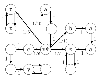
(a) directed graph with cycles

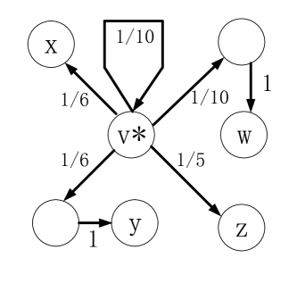
(b) directed graph with self-loops

Figure 1: Counter examples for submodularity.

Let $S:=\{x\}$, $T:=\{x,y\}$ and focus on node $v^{*}$. Then it is easy to check the following facts.

1. For any even time $t\geq 4$, $\mathbb{E}[X_{v^{*}}^{t}(S\cup\{z\})]-\mathbb{E}[X^{t}_{v^{*}}(S)]<\mathbb{E}[X_{v^{*}}^{t}(T\cup\{z\})]-\mathbb{E}[X^{t}_{v^{*}}(T)]$.

2. For any odd time $t\geq 5$, $\mathbb{E}[X^{t}_{v^{*}}(S\cup\{z\})]-\mathbb{E}[X^{t}_{v^{*}}(S)]=\mathbb{E}[X^{t}_{v^{*}}(T\cup\{z\})]-\mathbb{E}[X^{t}_{v^{*}}(T)]$.

This implies the function $A\mapsto\sum^{T}_{t=1}\mathbb{E}[X^{t}_{v^{*}}(A)]/T$ is not submodular when $T$ is large enough. ∎∎

      Theorem 4 (Networks with Self-loops).

There exists an information network in which the only directed cycle is a self-loop (on a non-void node), such that the according expected influence under NLT model is not submodular.

Proof.

Based on Theorem 2, it is sufficient to show that there exists an information network, which contains a node $v^{*}$, such that the function $A\mapsto\sum^{T}_{t=1}\mathbb{E}[X^{t}_{v^{*}}(A)]/T$ is not submodular. Actually, we only need to find a network in which there is a node $v^{*}$ and a particular time step $t$, such that $A\mapsto\mathbb{E}[X^{t}_{v^{*}}(A)]$ is not submodular. Consider the information network in Fig 1(b). Each edge $(v,u)$ is marked with the weight $b_{vu}$. Let $S:=\{x\}$, $T:=\{x,w,z\}$, and focus on node $v^{*}$. Then it is easy to check that for time $t=2$,

$$\mathbb{E}[X_{v^{*}}^{t}(S\cup\{y\})]-\mathbb{E}[X^{t}_{v^{*}}(S)]<\mathbb{E}[X_{v^{*}}^{t}(T\cup\{y\})]-\mathbb{E}[X^{t}_{v^{*}}(T)].$$

Thus, $A\mapsto\mathbb{E}[X^{2}_{v^{*}}(A)]$ is not submodular. ∎∎

5 Acyclic Information Networks

In this section, we consider the information networks without directed cycles. As we proved in Section 3, the influence maximization problem under NLT model is still NP-Hard even when the underlying network has no directed cycles.

Note that with the assumption of acyclic information networks, for any node $v\in V$ other than the void node, the set of its outgoing neighbors $\Gamma(v)$ has no directed path back to $v$. Intuitively, during the influence procedure, $v$’s choice of threshold $\theta_{v}$ can never affect the states of nodes in $\Gamma(v)$. To describe this fact formally, we introduce a random object on $\Omega$, where $\Omega$ is the sample space, which is essentially the set of all possible configurations of the thresholds.

      Definition 6 (States of Nodes over Time).

Suppose $\Omega$ is the sample space, and $W$ is a subset of nodes. Define a random object $\Pi_{W}:\Omega\rightarrow\{\mathcal{A},\mathcal{N}\}^{\mid W\mid\times T}$, such that for $\omega\in\Omega$, $v\in W$ and $1\leq t\leq T$, $\Pi_{W}(\omega)(v,t)$ indicates the state of node $v$ at time $t$ at the sample point $\omega$.

      Lemma 1 (Independence).

Suppose $v\in V$ and $\eta\in[0,1]$, and let $W$ be any subset of $V$ with no directed path to $v$. Then, we have $Pr[\theta_{v}\leq\eta\mid\Pi_{W}]=\eta$, under NLT model.

Proof.

In NLT model, the randomness comes from the choices of thresholds $\theta=\{\theta_{v}\}_{v\in V}$. The sample space is actually the set of all possible configurations of thresholds $\theta$.

Note that, the event $\theta_{v}\leq\eta$ is totally determined by the choice of $\theta_{v}$, and the value of $\Pi_{W}$ is totally determined by the choice of all $\theta_{u}$’s such that $u\neq v$. From the description of NLT model, the choices of thresholds are independent over different nodes. This implies that, for any $Q$ in the range of $\Pi_{W}$, the events $\theta_{v}\leq\eta$ and $\Pi_{W}=Q$ are independent.

Hence, we get $Pr[\theta_{v}\leq\eta\mid\Pi_{W}]=Pr[\theta_{v}\leq\eta]=\eta$. ∎∎

5.1 Connection to The Random Walk

Consider time $t>0$. The status of nodes at time $t$ may be associated, since they can share some common ancestors and the threshold of such an ancestor affects the status of its descendants. This association between different nodes cause more complicates for the analysis. In order to assist the analysis and handle the association carefully, we introduce a random walk process and show that this random walk process share an interesting connection with NLT model. Next, we introduce the random walk process.

      Model 2 (Random Walk Process (RW)).

Consider an information network $G=(V,E,b)$. For any given node $v\in V$, we define a random walk process as follows.

• At time $t=0$, the walk starts at node $v$.

• Suppose at some time $t$, the current node is $u$. A node $w\in\Gamma(u)$ is chosen with probability $b_{uw}$. The walk moves to node $w$ at time $t+1$.

      Definition 7 (Reaching Event).

For any node $v$, subset $C\subseteq V$ and $t\geq 0$, we use $R^{t}_{v}(C)$ to denote the event that a random walk starting from $v$ would reach a node in $C$ at precisely time $t$.

Next, we show the connection between the NLT model and the RW model for the case when the permanent initial set is empty. The more general case (arbitrary permanent initial set) will be considered later.

      Lemma 2 (Connection between NLT model and RW model).

Consider an acyclic information network $G$, and let $v$ be a non-void node, and $1\leq t\leq T$. On the same network $G$, consider the NLT process on a transient initial set $A$ and the RW process starting at $v$. Then, $\mathbb{E}[X^{t}_{v}(A)]=Pr[R^{t}_{v}(A)]$.

Proof.

This lemma is the key point in our argument, for which the proof is not obvious. To assist the proof of Lemma 2, we next introduce a process called “Path Effect” which is an “equivalent” presentation of the NLT model, and devote all the remaining part of this subsection to this lemma. ∎∎

We next introduce the PEprocess which augments the NLT model and defines (random) auxiliary array structures $P^{t}_{v}$ known as the influence paths to record the influence history. Intuitively, if $v$ becomes active at time $t$, then the path $P^{t}_{v}$ shows which of the initially active nodes is responsible. An important invariant is that node $v$ is active at time $t$ if and only if $P^{t}_{v}[0]\in A$.

      Model 3 (Path Effect Process (PE)).

Consider an information network $G=(V,E,b)$. Each node $v\in V$ is associated with a threshold $\theta_{v}$, which is chosen from $(0,1)$ uniformly at random.

Given a transient initial set $A\subseteq V$ and a configuration of the thresholds $\theta=\{\theta_{v}\}_{v\in V}$, for each node $v$ and each time step, the influence paths $P^{t}_{v}$ are constructed in the following influence procedure.

• At time $t=0$, for any $v\in V$, $P^{0}_{v}[0]=v$.

• At time $t>0$, define the active set at the previous time step as $A_{t-1}=\{u\in V\mid P^{t-1}_{u}[0]\in A\}$. For each node $v\in V$, we compute $f_{v}(A_{t-1}):=\sum_{u\in\Gamma(v)\cap A_{t-1}}b_{vu}$. Then,

  1. If $f_{v}(A_{t-1})\geq\theta_{v}$, choose node $u\in\Gamma(v)\cap A_{t-1}$ with probability $\frac{b_{vu}}{f_{v}(A_{t-1})}$;

  2. If $f_{v}(A_{t-1})<\theta_{v}$, choose node $u\in\Gamma(v)\setminus A_{t-1}$ with probability $\frac{b_{vu}}{1-f_{v}(A_{t-1})}$.

  Once $u$ is chosen, let $P^{t}_{v}[0,\ldots,t-1]:=P^{t-1}_{u}[0,\ldots,t-1]$ and $P^{t}_{v}[t]=u$.

      Remark 1.

Observe that given an information network with a transient initial set $A$ and a configuration $\theta$ of thresholds. Both of the NLT model and the PE process produce exactly the same active set $A_{t}$ at each time step $t$.

      Definition 8 (Source Event).

Consider an information network $G$ on which the PE process is run on the initial active set $A$. For any subset $C\subseteq V$, we use $I^{t}_{v}(C)$ to denote the event that $P^{t}_{v}[0]$ belongs to $C$. If $C\subseteq A$, this event means $v$’s state at time $t$ is the same as those of the nodes in $A$ at time 0 and hence is active. We shall see later on that the event $I^{t}_{v}(C)$ is independent of $A$ and hence the notation has no dependence on $A$.

When the given network is acyclic, the PE process has an interesting property.

      Lemma 3 (Acyclicity Implies Independence of Choice).

Consider an information network $G=(V,E,b)$ on which the PE process is run with some initial active set. If $G$ is acyclic, for any non-void node $v\in V$ and node $u\in\Gamma(v)$, we have $Pr[P^{t}_{v}[t]=u\mid\Pi_{W}]=b_{vu}$, where $W=\Gamma(v)$. Recall that $\Pi_{W}$ carries the information about the states of the nodes in $W$ at every time step.

Proof.

It is sufficient to prove that, for any value $Q$ in the range of $\Pi_{W}$, $Pr[P^{t}_{v}[t]=u\mid\Pi_{W}=Q]=b_{vu}$ holds. Because $f_{v}(A_{t-1})$ is determined by the states of $v$’s outgoing neighbors, once $Q$ is fixed, $\eta(Q)=f_{v}(A_{t-1})$ is determined. We consider two cases.

(1) When $u$ is in $A_{t-1}$ according to $Q$. We have

$Pr[P^{t}_{v}[t]=u\mid(\theta_{v}\leq\eta(Q))\cap(\Pi_{W}=Q)]=\frac{b_{vu}}{\eta(Q)}$.

Since $u\in A_{t-1}$ holds, the event $\{P^{t}_{v}[t]=u\}$ implies that $\{\theta_{v}\leq\eta(Q)\}$. Hence, we have

$$Pr[P^{t}_{v}[t]=u\mid\Pi_{W}=Q] = Pr[(P^{t}_{v}[t]=u)\cap(\theta_{v}\leq\eta(Q))\mid\Pi_{W}=Q]$$

$$= Pr[P^{t}_{v}[t]=u\mid(\theta_{v}\leq\eta(Q))\cap(\Pi_{W}=Q)]\cdot$$

$$Pr[\theta_{v}\leq\eta(Q)\mid\Pi_{W}=Q].$$

Because $G$ is acyclic, $W$ has no directed path to $v$. By Lemma 1, we have

$$Pr[\theta_{v}\leq\eta(Q)\mid\Pi_{W}=Q] = \eta(Q).$$

Hence, we have proved that $Pr[P^{t}_{v}[t]=u\mid\Pi_{W}=Q]=b_{vu}$.

(2) When $u$ is not in $A_{t-1}$ according to $Q$. The proof of this case is similar to the previous one. ∎∎

Recall the events $I^{t}_{v}(C)$ and $R^{t}_{v}(C)$ introduced in Definitions 8 and 7. The following lemma immediately implies Lemma 2 with $C=A$, and using the observation $\mathbb{E}[X^{t}_{v}(A)]=Pr[X^{t}_{v}(A)=1]=Pr[I^{t}_{v}(A)]$ from Remark 1.

      Lemma 4 (Connection between the PE process and the RW process).

Suppose the information network $G$ is acyclic, and $A$ is the transient initial set. For any $C\subseteq V$, any non-void node $v\in V$ and $t\geq 0$, we have $Pr[I^{t}_{v}(C)]=Pr[R^{t}_{v}(C)]$. In particular, the probability $Pr[I^{t}_{v}(C)]$ is independent of $A$.

Proof.

We use induction on $t$. For $t=0$, we have $Pr[I^{0}_{v}(C)]=1$ iff $v\in C$ and $Pr[R^{0}_{v}(C)]=1$ iff $v\in C$. Hence, $Pr[I^{0}_{v}(C)]=Pr[R^{0}_{v}(C)]$.

Suppose $Pr[I^{t}_{v}(C)]=Pr[R^{t}_{v}(C)]$ holds for all $v\in V$ at any time $t<k$.

We consider the case $t=k$ and fix some non-void node $v$. Let $W:=\Gamma(v)$. Recall that the random object $\Pi_{W}$ carries information about the states of all $v$’s outgoing neighbors at every time step. Let $\mathbb{C}^{k-1}_{u}$ be the set of the values for $\Pi_{W}$ under which $P^{k-1}_{u}[0]\in C$.

Observing that the events $\Pi_{W}=Q$ for different $Q$’s are mutually exclusive, we have

$$Pr[I^{k}_{v}(C)]=\sum_{u\in\Gamma(v)}\sum_{Q\in\mathbb{C}^{k-1}_{u}}Pr[\Pi_{W}=Q\mid P^{k}_{v}[k]=u]\cdot Pr[P^{k}_{v}[k]=u].$$

By Lemma 3, we have $Pr[P^{t}_{v}[t]=u\mid\Pi_{W}]=b_{vu}=Pr[P^{t}_{v}[t]=u]$, which implies for any value $Q$ of $\Pi_{W}$, it holds that $Pr[\Pi_{W}=Q\mid P^{k}_{v}[k]=u]=Pr[\Pi_{W}=Q]$. Consequently, we have

$$Pr[I^{k}_{v}(C)] = \sum_{u\in\Gamma(v)}\sum_{Q\in\mathbb{C}^{k-1}_{u}}Pr[\Pi_{W}=Q]\cdot Pr[P^{k}_{v}[k]=u]$$

$$= \sum_{u\in\Gamma(v)}Pr[I^{k-1}_{u}(C)]\cdot Pr[P^{k}_{v}[k]=u].$$

By induction hypothesis $Pr[I^{k-1}_{u}(C)]=Pr[R^{k-1}_{u}(C)]$, we get,

$$Pr[I^{k}_{v}(C)] = \sum_{u\in\Gamma(v)}Pr[R^{k-1}_{u}(C)]\cdot Pr[P^{k}_{v}[k]=u]$$

$$= \sum_{u\in\Gamma(v)}Pr[R^{k-1}_{u}(C)]b_{vu}.$$

The last term is just $R^{k}_{u}(C)$, according to the description of the RW process. This completes the inductive step of the proof. ∎∎

In the next subsection, we will reduce the general case with non-empty permanent initial set to the case when only transient initial set. Furthermore, we can prove the final conclusion (Theorem 6).

5.2 Submodularity of Acyclic NLT

At first, we consider the case where the permanent initial set $\widehat{A}$ is non-empty. We show that this general case can be reduced to the case where only transient initial set $A$ is non-empty, by the following transformation. Suppose $G$ is an information network, with transient initial set $A$ and permanent initial set $\widehat{A}$, and $T$ is the number of time steps to be considered. Consider the following transformation on the network instance. For each node $y\in\widehat{A}$, do the following:

1. Add a chain $D_{y}$ of $T$ dummy nodes to the network: starting from the head node of the chain, exactly one edge with weight 1 points to the next node, and so on, until the end node is reached.

2. Remove all outgoing edges from $y$. Add exactly one outgoing edge with weight 1 from $y$ to the head of the chain $D_{y}$

See Fig 2 for an example of the chain of dummy nodes.

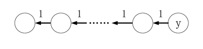
Figure 2: The chain of dummy nodes

Let $D:=\cup_{y\in\widehat{A}}D_{y}$ be the set of dummy nodes. We call the new network $\overline{G}(\widehat{A})$ the transformed network of $G$ with respect to $\widehat{A}$. When there is no risk of confusion, we simply write $\overline{G}$. The transformed instance on $\overline{G}(\widehat{A})$ only has $A\cup\widehat{A}\cup D$ as the transient initial set and no permanent initial node. The initially active dummy nodes in $D$ ensure that every node $y\in\widehat{A}$ is active for $T$ time steps. We use the notation convention that we add an overline to a variable (e.g., $\overline{X}$), if it is associated with the transformed network.

      Remark 2.

For any non-dummy, non-void node $v$,

$$X^{t}_{v}(A,\widehat{A})=\overline{X}^{t}_{v}(A\cup\widehat{A}\cup D).$$

      Lemma 5.

Suppose we are given an instance on information network $G$, with transient initial set $A$ and permanent initial set $\widehat{A}$. Let $v$ be any non-void node in $G$ and $0\leq t\leq T$. Suppose in the transformed network $\overline{G}(\widehat{A})$, for any subset $C$ of nodes in $G$, $\overline{R}^{t}_{v}(C)$ is the event that starting at $v$, the RWprocess on $\overline{G}$ for $t$ steps ends at a node in $C$. Then,

$$\mathbb{E}[X^{t}_{v}(A,\widehat{A})]=\sum_{u\in A}Pr[\overline{R}^{t}_{v}(\{u\})]+\sum_{y\in\widehat{A}}\sum^{t}_{i=0}Pr[\overline{R}^{i}_{v}(\{y\})].$$

Proof.

Let $v$ be a non-void node in $G$ and hence cannot be a dummy node in $\overline{G}$. By lemma 2, the equation $\mathbb{E}[X^{t}_{v}(A,\widehat{A})]=\mathbb{E}[\overline{X}^{t}_{v}(A\cup\widehat{A}\cup D)]$ implies

$$\mathbb{E}[X^{t}_{v}(A,\widehat{A})]=\sum_{u\in A}Pr[\overline{R}^{t}_{v}(\{u\})]+\sum_{y\in\widehat{A}}\left(Pr[\overline{R}^{t}_{v}(\{y\})]+\sum_{w\in D_{y}}Pr[\overline{R}^{t}_{v}(\{w\})]\right).$$

Consider the RW process on $\overline{G}$ starting at $v$. For any node $y\in\widehat{A}$, and consider a node $w\in D_{y}$ that is $i$ hops away from $y$. If $i>t$, then it is impossible for $v$ to reach $w$ in $t$ steps. Observe that if $v$ reaches $w$ at time $t$, then $v$ must reach $y$ at time $t-i$. Hence, $Pr[\overline{R}^{t}_{v}(\{w\})]=Pr[\overline{R}^{t-i}_{v}(\{y\})]$, and the summation over $i$ from 1 to $t$ gives the required formula. ∎∎

      Definition 9 (Passing-Through Event).

Let $G$ be an information network. For any node $v$, subset $C\subseteq V$ and $t\geq 0$, we use $S^{t}_{v}(C)$ to denote the event that a RW process on $G$ starting from $v$ would reach a node in $C$ at time $t$ or before.

      Lemma 6 (General Connection between the NLT model and the RW model).

Suppose $G$ is an acyclic information network, and let $v$ be a non-void node, and $1\leq t\leq T$. On the same network $G$, consider the NLT model with transient initial set $A$ and permanent initial set $\widehat{A}$, and the RW process starting at $v$. Then, $\mathbb{E}[X^{t}_{v}(A,\widehat{A})]=Pr[R^{t}_{v}(A)\cup S^{t}_{v}(\widehat{A})]$.

Proof.

Without loss of generality, we can still assume $A\cap\widehat{A}=\emptyset$, because $X^{t}_{v}(A,\widehat{A})=X^{t}_{v}(A\setminus\widehat{A},\widehat{A})$ and $R^{t}_{v}(A)\cup S^{t}_{v}(\widehat{A})=R^{t}_{v}(A\setminus\widehat{A})\cup S^{t}_{v}(\widehat{A})$. From Lemma 5, we have

$$\mathbb{E}[X^{t}_{v}(A,\widehat{A})]=\sum_{u\in A}Pr[\overline{R}^{t}_{v}(\{u\})]+\sum_{y\in\widehat{A}}\sum^{t}_{i=0}Pr[\overline{R}^{i}_{v}(\{y\})],$$

where the notation $\overline{R}$ means the corresponding term referring to the reaching event in the transformed graph $\overline{G}:=\overline{G}[\widehat{A}]$.

We compare the random walks of $t$ steps starting at $v$ on $G$ and on $\overline{G}$ using a coupling argument. Starting at $v$, the random walk on $\overline{G}$ copies the random choices made in $G$. This goes smoothly for the walk on $\overline{G}$ until a node $y$ in $\widehat{A}$ is hit, at which point further random choices made in $G$ are irrelevant. From this coupling argument, we can relate the events from $G$ and $\overline{G}$ in the following way:

• For $u\in A$, $Pr[\overline{R}^{t}_{v}(\{u\})]=Pr[R^{t}_{v}(\{u\})\setminus S^{t}_{v}(\widehat{A})]$.

• For $y\in\widehat{A}$, $\sum^{t}_{i=0}Pr[\overline{R}^{i}_{v}(\{y\})]$ is the probability that the walk in $G$ hits $y$ before any other node in $\widehat{A}$.

Hence, it follows that on the right hand side of (5.2), the first term is $Pr[Pr[R^{t}_{v}(A)\setminus S^{t}_{v}(\widehat{A})]$ and the second term is $Pr[S^{t}_{v}(\widehat{A})]$. Therefore, their sum is $Pr[R^{t}_{v}(A)\cup S^{t}_{v}(\widehat{A})]$, as required. ∎∎

      Theorem 5.

(Submodularity and Monotonicity of $\mathbb{E}[X^{t}_{v}(A,\widehat{A})]$). Consider the NLT model on an acyclic information network $G$ with transient initial set $A$ and permanent initial set $\widehat{A}$. Then, the function $(A,\widehat{A})\mapsto\mathbb{E}[X^{t}_{v}(A,\widehat{A})]$ is submodular and monotone.

Proof.

For notational convenience, we drop the superscript $t$ and the subscript $v$, and write for instance $X(A,\widehat{A}):=X^{t}_{v}(A,\widehat{A})$. For the reaching and the passing-through events associated with the Random Walk Process in $G$, we write $R(A):=R^{t}_{v}(A)$ and $S(A):=S^{t}_{v}(A)$

It is sufficient to prove that, for any $A\subseteq B\subseteq V$, $\widehat{A}\subseteq\widehat{B}\subseteq V$, and node $w\not\in(B\cup\widehat{B})$, the following inequalities hold:

$$\mathbb{E}[X(A\cup\{w\},\widehat{A})]-\mathbb{E}[X(A,\widehat{A})]\geq\mathbb{E}[X(B\cup\{w\},\widehat{B})]-\mathbb{E}[X(B,\widehat{B})];$$ (1)

$$\mathbb{E}[X(A,\widehat{A}\cup\{w\})]-\mathbb{E}[X(A,\widehat{A})]\geq\mathbb{E}[X(B,\widehat{B}\cup\{w\})]-\mathbb{E}[X(B,\widehat{B})].$$ (2)

By Lemma 6, for any subsets $C$ and $\widehat{C}$ such that $w\not\in(C\cup\widehat{C})$, $x(C\cup\{w\},\widehat{C})-x(C,\widehat{C})=Pr[R(C\cup\{w\})\cup S(\widehat{C})]-Pr[R(C)\cup S(\widehat{C})]=Pr[R(\{w\})\setminus S(\widehat{C})]$, where the last equality follows from definitions of reaching and passing-through events. Hence, inequality (1) follows because $\widehat{A}\subseteq\widehat{B}$ implies that $R(\{w\})\setminus S(\widehat{A})\supseteq R(\{w\})\setminus S(\widehat{B})$.

Similarly, $\mathbb{E}[X(C,\widehat{C}\cup\{w\})]-\mathbb{E}[X(C,\widehat{C})]=Pr[S(\{w\})\setminus(R(C)\cup S(\widehat{C}))]$. Hence, inequality (2) follows because $R(A)\cup S(\widehat{A})\subseteq R(B)\cup S(\widehat{B})$. ∎∎

      Corollary 1 (Objective Function is Submodular and Monotone).

With the same hypothesis as in Theorem 5, the function $(A,\widehat{A})\mapsto\overline{\sigma}(A,\widehat{A})$ is submodular and monotone.

At the end, we achieve the main result of this paper.

      Theorem 6.

Given an acyclic information network, a time period $[1,T]$, a budget $K$ and advertising costs (transient or permanent) that are uniform over the nodes, an advertiser can use the Standard Greedy Algorithm to compute a transient initial set $A$ and a permanent initial set $\widehat{A}$ with total cost at most $K$ in polynomial time such that $\overline{\sigma}(A,\widehat{A})$ is at least $\frac{1}{2}$ of the optimal value. Moreover, there is a randomized algorithm that outputs $A$ and $\widehat{A}$ such that the expected value (over the randomness of the randomized algorithm) of $\overline{\sigma}(A,\widehat{A})$ is at least $1-\frac{1}{e}$ of the optimal value, where $e$ is the natural number.

Proof.

We describe how Theorem 6 is derived. Recall that the advertiser is given a budget $K$, and the cost per transient node is $c$ and the cost per permanent node is $\widehat{c}$. Observe that if the advertiser uses $k$ transient nodes, where $k\leq\lfloor\frac{K}{c}\rfloor$, then there can be at most $\widehat{k}:=\lfloor\frac{K-kc}{\widehat{c}}\rfloor$ permanent nodes. Hence, for each such guess of $k$ and the corresponding $\widehat{k}$, the advertiser just needs to consider the maximization of the submodular and monotone function $(A,\widehat{A})\mapsto\overline{\sigma}(A,\widehat{A})$ on the matroid $\{(A,\widehat{A}):|A|\leq k,|\widehat{A}|\leq\widehat{k}\}$, for which $\frac{1}{2}$-approximation can be obtained in polynomial time using the techniques of Fisher et al. [12]. A randomized algorithm given by Calinescu et al. [3] achieves $(1-\frac{1}{e})$-approximation in expectation. ∎∎

References

- [1] C. Asavathiratham, S. Roy, B. Lesieutre, and G. Verghese. The influence model. Control Systems, IEEE, 21(6):52 –64, December 2001.
- [2] S. Bharathi, D. Kempe, and M. Salek. Competitive influence maximization in social networks. In Proceedings of the 3rd international conference on Internet and network economics, pages 306–311, 2007.
- [3] G. Călinescu, C. Chekuri, M. Pál, and J. Vondrák. Maximizing a monotone submodular function subject to a matroid constraint. SIAM J. Comput., 40(6):1740–1766, 2011.
- [4] T. Carnes, C. Nagarajan, S. M. Wild, and A. van Zuylen. Maximizing influence in a competitive social network: a follower’s perspective. In Proceedings of the 9th international conference on Electronic commerce, pages 351–360, 2007.
- [5] W. Chen, A. Collins, R. Cummings, T. Ke, Z. Liu, D. Rinc n, X. Sun, Y. Wang, W. Wei, and Y. Yuan. Influence maximization in social networks when negative opinions may emerge and propagate. In SDM, pages 379–390, 2011.
- [6] W. Chen, Y. Wang, and S. Yang. Efficient influence maximization in social networks. In Proceedings of the 15th ACM SIGKDD international conference on Knowledge discovery and data mining, pages 199–208, 2009.
- [7] W. Chen, Y. Yuan, and L. Zhang. Scalable influence maximization in social networks under the linear threshold model. In Proceedings of the 2010 IEEE International Conference on Data Mining, pages 88–97, 2010.
- [8] P. Domingos and M. Richardson. Mining the network value of customers. In Proceedings of the 7th ACM SIGKDD international conference on Knowledge discovery and data mining, pages 57–66, 2001.
- [9] P. Domingos and M. Richardson. Mining the network value of customers. In Proceedings of the seventh ACM SIGKDD international conference on Knowledge discovery and data mining, San Francisco, CA, USA, August 26-29, 2001, pages 57–66, 2001.
- [10] P. Dubey, R. Garg, and B. D. Meyer. Competing for customers in a social network. Department of Economics Working Papers 06-01, Stony Brook University, Department of Economics, 2006.
- [11] E. Even-Dar and A. Shapira. A note on maximizing the spread of influence in social networks. In Internet and Network Economics, volume 4858 of Lecture Notes in Computer Science, chapter 27, pages 281–286. Springer Berlin / Heidelberg, 2007.
- [12] M. L. Fisher, G. L. Nemhauser, and L. A. Wolsey. An analysis of approximations for maximizing submodular set functions. II. Math. Programming Stud., pages 73–87, 1978.
- [13] J. Goldenberg, B. Libai, and Muller. Using complex systems analysis to advance marketing theory development. Academy of Marketing Science Review, 2001.
- [14] J. Goldenberg, B. Libai, and E. Muller. Talk of the network: A complex systems look at the underlying process of Word-of-Mouth. Marketing Letters, pages 211–223, Aug. 2001.
- [15] M. Granovetter. Threshold models of collective behavior. The American Journal of Sociology, 83(6):1420–1443, 1978.
- [16] H. Hotelling. Stability in competition. The Economic Journal, 39(153):pp. 41–57, 1929.
- [17] S. Jurvetson. What exactly is viral marketing?
- [18] D. Kempe, J. Kleinberg, and É. Tardos. Maximizing the spread of influence through a social network. In Proceedings of the ninth ACM SIGKDD international conference on Knowledge discovery and data mining, pages 137–146. ACM, 2003.
- [19] D. Kempe, J. Kleinberg, and E. Tardos. Influential nodes in a diffusion model for social networks. In Proceedings of the 32nd International Colloquium on Automata, Languages and Programming, pages 1127–1138, 2005.
- [20] J. Leskovec, A. Krause, C. Guestrin, C. Faloutsos, J. VanBriesen, and N. Glance. Cost-effective outbreak detection in networks. In Proceedings of the 13th ACM SIGKDD international conference on Knowledge discovery and data mining, pages 420–429, 2007.
- [21] E. Mossel and S. Roch. On the submodularity of influence in social networks. In Proceedings of the 39th annual ACM symposium on Theory of computing, pages 128–134, 2007.
- [22] G. L. Nemhauser, L. A. Wolsey, and M. L. Fisher. An analysis of approximations for maximizing submodular set functions I. Mathematical Programming, 14(1):265–294, Dec. 1978.
- [23] S. Wasserman and K. Fraust. Social Network Analysis. Cambridge University Press, 1994.