Ice Nucleation on Carbon Surface Supports the Classical Theory for Heterogeneous Nucleation

Abstract

The prevalence of heterogeneous nucleation in nature was explained qualitatively by the classical theory for heterogeneous nucleation established over more than 60 years ago, but the quantitative validity and the key conclusions of the theory have remained unconfirmed. Employing the forward flux sampling method and the coarse-grained water model mW, we explicitly computed the heterogeneous ice nucleation rates in the supercooled water on a graphitic surface at various temperatures. The independently calculated ice nucleation rates were found to fit well according to the classical theory for heterogeneous nucleation. The fitting procedure further yields the estimate of the potency factor which measures the ratio of the heterogeneous nucleation barrier to the homogeneous nucleation barrier. Remarkably, the estimated potency factor agrees quantitatively with the volumetric ratio of the critical nuclei between the heterogeneous and homogeneous nucleation. Our numerical study thus provides a strong support to the quantitative power of the theory, and allows understanding ice nucleation behaviors under the most relevant freezing conditions.

The freezing of water nearly all proceeds with the assistance from foreign substances, a process known as heterogeneous nucleation. In clouds, the dominant candidates for heterogeneous ice nucleation are bacteria, pollen grains, mineral dusts, soot particles, and high-molecular-weight organic compounds Cantrell and Heymsfield (2005); Murray et al. (2012). Despite its ubiquity, the microscopic picture behind such prevailing process still remains elusive, because of the complex and stochastic nature of the heterogeneous nucleation event. In particular, the mechanisms controlling heterogeneous ice nucleation are not well understood.

Although a molecular understanding is still missing, the thermodynamic rationale behind the heterogeneous nucleation was already provided in 1950’s by the classical theory for heterogeneous nucleation Turnbull (1950a, b), an extension to the classical nucleation theory (CNT) Volmer and Weber (1926) for homogeneous nucleation, on the basis of macroscopic arguments. According to CNT, the formation of a critical nucleus needs to overcome a free energy barrier $\Delta G^{*}_{\text{hom}}$ through spontaneous fluctuations. In the case of a spherical solid nucleus forming from the supercooled liquid, the free energy barrier can be expressed as

$$\Delta G^{*}_{\text{hom}}=\frac{16\pi\gamma_{ls}^{3}}{3(\rho\Delta\mu_{ls})^{2}}\;,$$ (1)

where $\gamma_{ls}$ is the solid-liquid interface free energy, $\Delta\mu_{ls}$ is the chemical potential difference between liquid and solid, and $\rho$ is the density of liquid. The homogeneous nucleation rate $R_{\text{hom}}$ varies with the nucleation temperature $T$ following the Arrhenius equation Kelton (1991):

$$R_{\text{hom}}=A_{\text{hom}}\;\exp(-\Delta G^{*}_{\text{hom}}/k_{B}T)\;,$$ (2)

where $A_{\text{hom}}$ is the kinetic pre-factor. For homogeneous ice nucleation, both experiments Kramer et al. (1999); Koop et al. (2000); Stockel et al. (2005); Taborek (1985); Murray et al. (2010) and simulations Li et al. (2011, 2013); Moore and Molinero (2011); Reinhardt and Doye (2012); Sanz et al. (2013); Espinosa et al. (2014) suggest that the temperature dependence of the homogeneous ice nucleation rate may be quantitatively described by CNT, with parametrization being refined by the controlled experiments Koop and Zobrist (2009).

When a foreign flat wall (W) is present, the solid nucleus can preferentially form at the interface between the liquid and the wall (Fig. 1(a)). At its critical size, the solid embryo is under the unstable equilibrium with respect to the dissolution and the growth, which also indicates a mechanical equilibrium. At the liquid-solid-wall triple junction, solving the equation of equilibrium yields the Young’s equation

$$\gamma_{lw}=\gamma_{sw}+\gamma_{ls}\cos\theta_{c}\;,$$ (3)

where $\gamma_{lw}$ and $\gamma_{sw}$ are the surface tensions for liquid-wall and solid-wall interfaces. $\theta_{c}$ defines the contact angle of solid embryo on the flat wall, with $\theta_{c}=0$ and $\theta_{c}=180^{o}$ indicating the complete wetting of the wall by solid and liquid, respectively. If the solid nucleus is further assumed to be part of the sphere, i.e., a spherical cap, its volume $V_{\text{cap}}$ can be expressed as $V_{\text{cap}}=f(\theta_{c})V_{\text{sphere}}$, where

$$f(\theta_{c})=(1-\cos\theta_{c})^{2}(2+\cos\theta_{c})/4\;,$$ (4)

and $V_{\text{sphere}}$ is the volume of the sphere containing the cap. Remarkably, under the framework of classical theory for heterogeneous nucleation, the factor $f(\theta_{c})$ coincides with the ratio of the free energy barriers between the heterogeneous and homogeneous nucleation, i.e., $f(\theta_{c})=\Delta G^{*}_{\text{het}}/\Delta G^{*}_{\text{hom}}$. It thus follows that

$$f(\theta_{c})=\frac{\Delta G^{*}_{\text{het}}}{\Delta G^{*}_{\text{hom}}}=\frac{V_{\text{cap}}}{V_{\text{sphere}}}$$ (5)

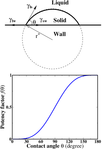
Figure 1: (a) A solid critical nucleus forms at the interface between liquid and a foreign flat wall, with a solid contact angle $\theta_{c}$. The contact angle $\theta_{c}$ can be determined by the surface tensions through Eqn. (3). The solid nucleus is assumed to be part of a sphere (dashed line) with a radius $r^{*}$, i.e., a spherical cap with the volume $V_{\text{cap}}=f(\theta_{c})V_{\text{sphere}}$. (b) The potency factor $f(\theta_{c})$ increases from 0 to 1 (homogeneous), as the solid contact angle $\theta_{c}$ varies from 0 to $180^{o}$.

Eqn. (5) provides a simple but robust explanation for the preference of the heterogeneous nucleation over the homogeneous nucleation: Instead of forming a spherical nucleus from spontaneous thermal fluctuations, only part of the sphere $V_{\text{cap}}$ needs to be nucleated when a foreign surface is present. Accordingly, the free energy barrier is reduced by the same factor $f(\theta_{c})$ by which the volume of critical nucleus is reduced. Since $f(\theta_{c})$ measures the degree of the free energy reduction, it is also known as the potency factor. According to Eqn. (4), the potency factor $f(\theta_{c})$ for a foreign wall is determined by the solid contact angle $\theta_{c}$, and varies between 0 and 1, as shown in Fig. 1(b). A wall with a lower solid contact angle yields a lower potency factor $f(\theta_{c})$, thus further enhancing heterogeneous nucleation. Then the heterogeneous nucleation rate can be expressed by

$$R_{\text{het}}=A_{\text{het}}\;\exp(-f(\theta_{c})\Delta G^{*}_{\text{hom}}/k_{B}T)\;,$$ (6)

Although the classical theory for heterogeneous nucleation offers a qualitative explanation to the prevalence of heterogeneous nucleation, its quantitative validity remains unconfirmed. Auer and Frenkel Auer and Frenkel (2003) employed umbrella sampling method to calculate the nucleation barrier of the hard-sphere crystal that completely wets the smooth walls, and found that the computed barrier height is substantially higher than that predicted by the CNT. The disagreement was attributed to the omission in the CNT of the line tension at the liquid-solid-wall triple junction, which may become non-negligible when crystal completely wets the wall. In a recent study by Winter et. al.Winter et al. (2009), the total surface energies of the liquid nuclei (of both spherical and spherical cap shape) were directly obtained by Monte Carlo simulation for the Ising lattice gas model. It was found that the obtained surface energies could be comparable with the capillary approximation employed by CNT, if the line tension effects at the triple junction are considered.

In this work, we show that the heterogeneous ice nucleation on a graphitic surface indeed supports the quantitative power of the theory. In particular, the validity of Eqn. (5) and (6) is strongly supported from the ice nucleation rates computed explicitly using the forward flux sampling method over a wide temperature range. Our work thus provides the first validation of heterogeneous CNT in the partially wetting regime where the potency factor is far enough from zero.

Our molecular dynamics (MD) simulations were carried out using the coarse-grained model of water (mW) Molinero and Moore (2009). The inter-molecular interaction between water and carbon was adopted from a recent parameterization of the two-body term of the mW model, so that the strength of the water-carbon interaction reproduces the experimental contact angle ($86^{o}$) of water on graphite Lupi et al. (2014). The model was recently employed in direct MD simulations to study the heterogeneous ice nucleation on carbon surface Lupi et al. (2014); Lupi and Molinero (2014); Reinhardt and Doye (2014), where the nonequilibrium freezing temperature of ice was found to increase due to the preferential nucleation of ice on carbon surface. Here we employ the forward flux sampling (FFS) method Allen et al. (2006a, b) to systematically and explicitly compute the heterogeneous ice nucleation rates at various temperatures where spontaneous ice nucleation becomes too slow to occur in direct simulation. The details of the rate constant calculations can be found in the Supplementary Materials. Our MD simulation includes 4096 water molecules and 1008 carbon atoms, in a nearly cubic cell with a periodic boundary condition. The isobaric-isothermal canonical ensemble (NPT) with a No$\acute{\mbox{s}}$e-Hoover thermostat was employed, with a relaxation time of 1 ps and 15 ps for temperature and pressure, respectively. A time step of 5 fs was used. It should be noted that while the homogeneous nucleation rate is measured by the nucleation frequency per unit volume, the heterogeneous nucleation rate should be characterized by the nucleation frequency per unit area. However because the simulation volume of liquid is small, and ice nucleation on carbon surface is strongly preferred, it is convenient to describe the heterogeneous nucleation rate $R_{\text{het}}$ on the basis of volume, in order to facilitate a direct comparison with $R_{\text{hom}}$.

Figure 2 shows the computed heterogeneous ice nucleation rates (in logarithm) as a function of nucleation temperature, in the range of 220 K to 240 K. To quantitatively explore the catalytic activity of the graphitic surface, we compare the obtained heterogeneous ice nucleation rates with the reported homogeneous ice nucleation rates from the previous work Li et al. (2011) using the FFS method and the mW water model, as shown in Figure 2. It is clear that a graphitic surface yields the significantly enhanced ice nucleation rates, under all temperatures studied. Our results thus support the finding by Lupi at. al. Lupi et al. (2014) and confirm the enhanced ice nucleation capacity of carbon surface.

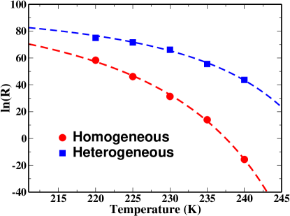
Figure 2: Temperature dependence of ice nucleation rate (logarithm) in the mW water model, for both homogeneous ice nucleation (red) and the heterogeneous nucleation on a graphitic surface (blue). The solid red dots and blue squares represent the calculated ice nucleation rates by using the FFS method. The dashed red and blue lines indicate the fitting, on the basis of the CNT for homogeneous nucleation (Eqn. (7)) and the extension for heterogeneous nucleation (Eqn. (8)), respectively. The data of homogeneous nucleation were extracted from Ref. Li et al. (2011).

The calculated heterogeneous ice nucleation rates at various temperatures allow assessing the quantitative validity of Eqn. (6). To do this, we fit the obtained heterogeneous ice nucleation rates at various temperatures according to the theory of nucleation, using the procedure employed by Li at. al. in analyzing the homogeneous ice nucleation Li et al. (2011). In this procedure, the chemical potential difference $\Delta\mu$ is approximated as a linear function of temperature, i.e., $\Delta\mu=H(T-T_{m})/T_{m}$, where $T_{m}$ is the equilibrium melting temperature (274.6 K) of ice in the mW model, and $H$ is a constant; The liquid-solid interface energy $\gamma_{ls}$ is assumed to be temperature independent. It is noted that both assumptions have been verified for the mW water model in different simulation studies Espinosa et al. (2014); Jacobson et al. (2009). For homogeneous ice nucleation, it was shown that the independently calculated homogeneous ice nucleation rate can be fitted according to the following expression:

$$\ln(R_{\text{hom}})=\ln(A_{\text{hom}})+\frac{C_{\text{hom}}}{(T-T_{m})^{2}T}\;,$$ (7)

where $\ln(A_{\text{hom}})=114.07\pm 1.86$ and $C_{\text{hom}}=-16\pi\gamma_{ls}^{3}T_{m}^{2}/(3k_{B}\rho^{2}H^{2})=-3.72\pm 0.08\times 10^{7}$ K³ are the fitting constants Li et al. (2011). We note that the nucleation barrier $\Delta G^{*}_{\text{hom}}=k_{B}C_{\text{hom}}/(T-T_{m})^{2}$. The fitting yielded an estimate of $\gamma_{ls}=31.01\pm 0.21$ mJ m^-2, which agrees well with the surface tensions computed through other approaches for the mW water model Limmer and Chandler (2012); Espinosa et al. (2014).

Remarkably, the obtained heterogeneous ice nucleation rates are also found to fit well the classical theory for heterogeneous nucleation, as shown in Figure 2. Specifically, the calculated ice nucleation rates $R_{\text{het}}$ can be fitted according to

$$\ln(R_{\text{het}})=\ln(A_{\text{het}})+\frac{C_{\text{het}}}{(T-T_{m})^{2}T}\;.$$ (8)

The fitting yields the estimate of the kinetic pre-factor for heterogeneous nucleation $\ln(A_{\text{het}})=102\pm 7.70$, which is consistent with that for the homogeneous nucleation $\ln(A_{\text{hom}})=114.07\pm 1.86$ Li et al. (2011). More importantly, the other fitting constant $C_{\text{het}}=-1.70\pm 0.07\times 10^{7}$ K³ allows estimating the reduction of the nucleation barrier, as $C_{\text{het}}/C_{\text{hom}}=\Delta G^{*}_{\text{het}}/\Delta G^{*}_{\text{hom}}\equiv f_{b}(\theta_{c})$. By comparing the fitting constants $C$ from the heterogeneous and homogeneous ice nucleation, we obtain the potency factor for the graphitic surface $f_{b}(\theta_{c})=0.456\pm 0.019$. This corresponds to a solid contact angle of $\theta_{c}\sim 86.6^{o}$. It is noted here that $\theta_{c}$ is the contact angle between ice and graphene, and should not be confused with the water-graphene contact angle $86^{o}$, although their magnitudes coincide here.

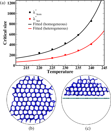
Figure 3: (a) Variation of the critical ice nucleus size with temperature for both homogeneous and heterogeneous nucleation. The critical size is estimated based on the committor probability analysis, which yields $\lambda^{*}_{\text{het}}$: $145\pm 5$ at 225 K, $205\pm 10$ at 230 K, $288\pm 7$ at 235 K, and $410\pm 10$ at 240 K, respectively (See Supplementary Materials for more details). The critical size for homogeneous nucleation was obtained in Ref. Li et al. (2011). The simulation data and the fitted curves are represented by data points and solid lines, respectively. (b) A snap shot of the critical ice nucleus forming from homogeneous ice nucleation at 240 K. (c) A snap shot of the critical ice nucleus forming on graphene surface at 240 K.

It is then of interest to further test the validity of Eqn. (5), namely, the potency factor $f_{b}(\theta_{c})$ can be also quantitatively related to the volumetric ratio $f_{v}(\theta_{c})$ of the critical nucleus of the heterogeneous nucleation and the homogeneous nucleation. We note that such verification becomes possible in our study because the size of the critical nucleus $\lambda^{*}$ can be independently estimated from the ensemble of nucleation trajectories obtained in the FFS calculation. Using the definition that the critical nucleus has the equal probabilities of dissolving and growing completely, i.e., with a committor probability $p_{\mbox{B}}=0.5$ Bolhuis et al. (2002), we obtained the estimate of the critical nucleus size $\lambda$ (number of water molecules contained in the critical ice nucleus) at various nucleation temperatures, as shown in Fig. 3. According to CNT, the critical size of the spherical nucleus in homogeneous nucleation is expressed by $\lambda^{*}_{\text{hom}}=32\pi\gamma^{3}/(3\rho^{2}(\Delta\mu)^{3})$. For mW water model, since $\gamma$ is nearly temperature independent and $\Delta\mu=H(T-T_{m})/T_{m}$ Espinosa et al. (2014), the critical size $\lambda^{*}_{\text{hom}}$ exhibits the following temperature dependence:

$$\lambda^{*}_{\text{hom}}(T)=\frac{32\pi\gamma^{3}}{3\rho^{2}H^{3}}\frac{1}{\left(\frac{T_{m}}{T}-1\right)^{3}}=\frac{B_{\text{hom}}}{\left(\frac{T_{m}}{T}-1\right)^{3}}\;,$$ (9)

where $B_{\text{hom}}$ is the temperature independent constant. The obtained critical size $\lambda^{*}_{\text{hom}}$ at various temperatures are found to fit well according to Eqn (9), as shown in Fig. 3(a). The good fit is not unexpected because previous studies Reinhardt and Doye (2012); Li et al. (2013) have shown the critical ice nucleus from homogeneous nucleation is nearly spherical. The fitting procedure yields the constant $B_{\text{hom}}=1.752\pm 0.027$. For the heterogeneous ice nucleation, the same fitting procedure was found to equivalently apply to the calculated critical nucleus size $\lambda^{*}_{\text{het}}$, through

$$\lambda^{*}_{\text{het}}(T)=\frac{B_{\text{het}}}{\left(\frac{T_{m}}{T}-1\right)^{3}}\;,$$ (10)

which yields the constant $B_{\text{het}}=0.840\pm 0.014$. By comparing the two fitting constants $B$, one obtains the volumetric ratio $f_{v}(\theta_{c})\equiv\lambda^{*}_{\text{het}}/\lambda^{*}_{\text{hom}}=B_{\text{het}}/B_{\text{hom}}$. Remarkably, the obtained volumetric ratio $f_{v}(\theta_{c})=0.480\pm 0.011$ agrees quantitatively with the potency factor $f_{b}(\theta_{c})=0.456\pm 0.019$ estimated from the nucleation barriers. The quantitative validity of Eqn. (5), an important conclusion from CNT and its extension, is thus strongly supported through the molecular simulation results based on the mW water model.

The verified quantitative validity of the CNT (and its extension) then allows predicting ice nucleation behavior in the presence of a heterogeneous nucleation center. The nucleation efficacy of the foreign surface can be generally described based on its potency factor $f$. Using the fitted kinetic pre-factor $A_{\text{hom}}$ ($\approx A_{\text{het}}$) and $C_{\text{hom}}$, and Eqn. (8), one obtains both the heterogeneous ice nucleation rate and the corresponding critical nucleus size, as a function of the nucleation temperature, for different potency factors $f$. As shown in Fig. 4, the predicted ice nucleation rates clearly indicate the preference and the relevance of the heterogeneous nucleation at the moderate and low supercooling. For example, at 250 K, a nucleation center with the potency factor of $f=0.1$ (equivalent to a solid contact angle $\theta_{c}=52.5^{o}$) yields an ice nucleation rate about 100 orders of magnitude higher than that of homogeneous nucleation at the same temperature. Intriguingly, the sizes of the critical nuclei from these relevant nucleation events fall within the range of a few hundred to a few thousand water molecules. This implies that the most relevant ice nucleation events mediated by an effective nucleation center under a low supercooling, i.e., $-10^{o}\text{C}\sim-20^{o}\text{C}$, can be possibly modeled by molecular simulations through using a reasonable number ($10^{3}\sim 10^{4}$) of water molecules.

Figure 4: The predicted temperature variation of (a) ice nucleation rate $R(T)$ and (b) critical size of ice nucleus $\lambda^{*}(T)$ in the mW water model, due to the presence of a heterogeneous nucleation center with different potency factor $f$. A small potency factor $f$ indicates a strong ice nucleation efficacy, and $f=1$ corresponds to homogeneous ice nucleation. (c) The predicted variation of the critical size $\lambda^{*}$ for different potency factor $f$, subject to a fixed nucleation rate.

Interestingly, when ice nucleation rate $R$ is fixed, the theory of nucleation predicts that the critical size $\lambda^{*}$ decreases with the potency factor $f$ (Fig. 4(c)), and a homogeneous nucleation yields the minimum critical nucleus. This may appear surprising, but the prediction can be understood by the fact that the heterogeneous nucleation producing the same ice nucleation rate occurs at a much elevated temperature (Fig. 4(a)). For example, an ice nucleation rate of $10^{20}\;\mbox{m}^{-3}\mbox{s}^{-1}$ would require a homogeneous nucleation temperature $T_{\text{hom}}\approx 225$ K, but a heterogeneous nucleation temperature $T_{\text{het}}\approx 260$ K for the nucleation center with a potency factor $f=0.1$. The prediction (Fig. 4(c)) shows the critical nucleus for such heterogeneous nucleation at 260 K contains about 1220 water molecules (i.e., 1/10 of the critical size of the homogeneous nucleation at 260 K), larger than the critical size (310) of the homogeneous nucleation at 225 K. As the solid contact angle $\theta_{c}$ decreases with the nucleation efficacy (Fig. 1), a strong ice nucleation center yields a more “flat” ice nucleus that appears increasingly two-dimension like. It is noted that in such scenario the possible effect from the line tension at the triple junction can be non-negligible Auer and Frenkel (2003); Winter et al. (2009). However its quantitative effect in ice nucleation rate is unclear. Using the density of ice, one can estimate the radius of the spherical segment (i.e., the frustum of the spherical cap) to be of the order of a few nano meters, implying that the dimension of an effective ice nucleation site is typically of the order of $10^{1}$ nm. This estimate may be used as an important parameter in experiments for potentially observing ice nucleation in situ and designing effective strategy for controlling ice nucleation.