Deviation from power law of the global seismic moment distribution

Abstract

The distribution of seismic moment is of capital interest to evaluate earthquake hazard, in particular regarding the most extreme events. We make use of likelihood-ratio tests to compare the simple Gutenberg-Richter power-law distribution with two statistical models that incorporate an exponential tail: the so-called tapered Gutenberg-Richter and the truncated gamma, when fitted to the global CMT earthquake catalog. The outcome is that the truncated gamma model outperforms the other two models. If simulated samples of the truncated gamma are reshuffled in order to mimic the time occurrence of the order statistics of the empirical data, this model turns out to be able to explain the empirical data both before and after the great Sumatra-Andaman earthquake of 2004.

The Gutenberg-Richter (GR) law is not only of fundamental importance in statistical seismology Utsu_GR but also a cornerstone of non-linear geophysics Malamud_hazards and complex-systems science Bak_book . It simply states that, for a given region, the magnitudes of earthquakes follow an exponential probability distribution. As the (scalar) seismic moment is an exponential function of magnitude, when the GR law is expressed in terms of the former variable, it translates into a power-law distribution Knopoff_Kagan77 ; Corral_Lacidogna , i.e.,

$$f(M)\propto\frac{1}{M^{1+\beta}},$$ (1)

with $M$ seismic moment, $f(M)$ its probability density, (fulfilling $\int_{\forall M}f(M)dM=1$), the sign “$\propto$” denoting proportionality, and the exponent $1+\beta$ taking values close to 1.65. This simple description provides rather good fits of available data in many cases Kagan_pageoph99 ; Kagan_gji02 ; Corral_Deluca ; Kagan_book , with, remarkably, only one free parameter, $\beta$. A totally equivalent characterization of the distribution uses the survivor function (or complementary cumulative distribution), defined as $S(M)=\int_{M}^{\infty}f(M^{\prime})dM^{\prime}$, for which the GR power law takes the form $S(M)\propto 1/M^{\beta}$.

The power-law distribution has important physical implications, as it suggests an origin from a critical branching process or a self-organized-critical system Bak_book ; Vere_Jones76 ; Main . Nevertheless, it presents also some conceptual difficulties, due to the fact that the mean value $\langle M\rangle$ provided by the distribution turns out to be infinite Knopoff_Kagan77 . These elementary considerations imply that the GR law cannot be naively extended to arbitrarily large values of $M$, and one needs to introduce additional parameters to describe the tail of the distribution, coming presumably from finite-size effects. However, a big problem is that the change from power law to a faster decay seems to take place at the highest values of $M$ that have been observed, for which the statistics are very poor Zoller_grl .

Kagan Kagan_gji02 has enumerated the requirements that an extension of the GR law should fulfill; in particular, he considered, among other: (i) the so called tapered (Tap) Gutenberg-Richter distribution (also called Kagan distribution Vere_Jones_gji ), with a survivor function given by $S_{tap}(M)\propto e^{-M/\theta}/M^{\beta}$ and (ii) the (left-) truncated gamma (TrG) distribution, for which the density is $f_{trg}(M)\propto e^{-M/\theta}/M^{1+\beta}$. Note that both expressions have essentially the same functional form, but the former refers to the survivor function and the later to the density. As, in general, $f(M)=-dS(M)/dM$, differentiation of $S_{tap}(M)$ in (i) shows the difference between both distributions. In any case, parameter $\theta$ represents a crossover value of seismic moment, signaling a transition from power law to exponential decay; so, $\theta$ gives the scale of the finite-size effects on the seismic moment. The corresponding value of (moment) magnitude (sometimes called corner magnitude) can be obtained from $m_{c}=\frac{2}{3}\left(\log_{10}\theta-9.1\right)$, when the seismic moment is measured in N$\cdot$m Kanamori_77 ; Kanamori_rpp .

Kagan Kagan_gji02 also argues that available seismic catalogs do not allow the reliable estimation of $\theta$, except in the global case (or for large subsets of this case), in particular, he recommends the use of the centroid moment tensor (CMT) catalog Ekstrom2012 . From his analysis of global seismicity, and comparing the values of the likelihoods, Kagan Kagan_gji02 concludes that the tapered GR distribution gives a slightly better fit than the truncated gamma distribution, for which in addition the estimation procedure is more involving. In any case, the $\beta-$value seems to be universal (at variance with $\theta$), see also Refs. Kagan_book ; Godano_pingue ; Kagan_tectono10 .

Nevertheless, the data analyzed by Kagan Kagan_gji02 , from 1977 to 1999, comprises a period of relatively low global seismic activity, with no event above magnitude 8.5; in contrast, the period 1950 – 1965 witnessed 7 of such events Lay . Starting with the great Sumatra-Andaman earthquake of 2004, and following since then with 4 more earthquakes with $m\geq 8.5$, the current period seems to correspond to the past higher levels of activity (up to the time of submitting this letter). Main et al. and Bell et al. Main_ng ; Bell_Naylor_Main have re-examined the problem of the seismic moment distribution including recent global data (shallow events only). Using a Bayesian information criterion (BIC), Bell et al. Bell_Naylor_Main compare the plain GR power law with the tapered GR distribution, and conclude that, although the tapered GR gives a significantly better fit before the 2004 Sumatra event, the occurrence of this changes the balance of the BIC statistics, making the GR power law more suitable; that is, the power law is more parsimonious, or simply, is enough for describing global shallow seismicity when the recent mega-earthquakes are included in the data. Similar results have been published in Ref. Geist_Parsons_NH .

In this paper we revisit the problem with more recent data, using other statistical tools, reaching somewhat different conclusions. As in the mentioned papers, we analyze the global CMT catalog Ekstrom2012 , in our case for the period between 1 January 1977 and 31 October 2013, with the values of the seismic moment converted into N$\cdot$m ($1$ dyn$\cdot$cm $=10^{-7}$ N$\cdot$m). We restrict to shallow events (depth $<70$ km) and in order to avoid incompleteness, to magnitude $m>5.75$ (equivalent to $M>5.3\cdot 10^{17}$ N$\cdot$m), as in Refs. Main_ng ; Bell_Naylor_Main . This yields $6150$ events.

As statistical tools, we use maximum likelihood estimation (MLE) for fitting, and likelihood ratio (LR) tests for comparison of different fits. Model selection tests based on the likelihood ratio have the advantage that the ratio is invariant with respect to changes of variables (if these are one-to-one Pawitan2001 ). Moreover, for comparing the fit of models in pairs, LR test is preferable in front of the computation of differences in BIC or AIC (Akaike information criterion), as the test relies on the fact that the distribution of the LR is known, under a suitable null hypothesis (although the log-likelihood-ratio is equal to the difference of BIC or AIC when the number of parameters of the two models is the same).

Maximum likelihood estimation is the best-accepted method in order to fit probability distributions, as it yields estimators which are invariant under re-parameterizations, and which are asymptotically unbiased and efficient for regular models, in particular for exponential families Pawitan2001 . When maximum likelihood is used under a wrong model, what one finds is the closest model to the true distribution in terms of the Kullback-Leibler distance Pawitan2001 . In order to perform MLE it is necessary to specify the densities of the distributions, including the normalization factors. In our case, all distributions are defined for $M$ above the completeness threshold $a$, i.e., for $M>a$, being zero otherwise (as mentioned above, $a$ is fixed to $5.3\cdot 10^{17}$ N$\cdot$m). For the power-law (PL) distribution (which yields the GR law for the distribution of $M$) Eq. (1) reads

$$f_{pl}(M;\beta)=\frac{\beta}{a}\left(\frac{a}{M}\right)^{1+\beta},$$

with $\beta>0$. For the tapered Gutenberg-Richter,

$$f_{tap}(M;\beta,\theta)=\left[\frac{\beta}{a}\left(\frac{a}{M}\right)^{1+\beta}+\frac{1}{\theta}\left(\frac{a}{M}\right)^{\beta}\right]e^{-(M-a)/\theta},$$

with $\beta>0$ and $\theta>0$. And for the left-truncated (and extended to $\beta>0$) gamma distribution;

$$f_{trg}(M;\beta,\theta)=\frac{1}{\theta\Gamma(-\beta,a/\theta)}\left(\frac{\theta}{M}\right)^{1+\beta}e^{-M/\theta},$$

with $-\infty<\beta<\infty$ and $\theta>0$, and with $\Gamma(\gamma,z)=\int_{z}^{\infty}x^{\gamma-1}e^{-x}dx$ the upper incomplete gamma function, defined for $z>0$ when $\gamma<0$. We summarize the parameterization of the densities as $f(M;\Theta)$, where $\Theta=\{\beta,\theta\}$ for the Tap and TrG distributions and $\Theta=\beta$ for the power law. Note that for the TrG distribution, it is clear that the exponent $\beta$ is a shape parameter and $\theta$ is a scale parameter; in fact, these parameters play the same role in the Tap distribution, which turns out to be a mixture of two truncated gamma distributions, one with shape parameter $\beta$ and the other with $\beta-1$, but with common scale parameter $\theta$. In contrast, the power law lacks a scale parameter. In all cases the completeness threshold $a$ is a truncation parameter, but it is kept fixed and is not a free parameter, therefore.

The knowledge of the probability densities allows the direct computation of the likelihood function as $L(\Theta)=\prod_{i=1}^{N}f(M_{i};\Theta),$ where $M_{i}$ are the $N$ observational values of the seismic moment. Maximization of the likelihood function with respect the values of the parameters leads to the maximum-likelihood estimation $\hat{\Theta}$ of these parameters, with $\hat{L}=L(\hat{\Theta})$ the value of the likelihood at its maximum. We perform the MLE for the 3 models, obtaining, for the complete datasets, the values reported in Table 1.

		$\hat{\beta}$	$\hat{\theta}$ (N$\cdot$m)	$\hat{m}_{c}$	$l$ ($M$ in N$\cdot$m)
PL	MLE	0.685	$\infty$	$\infty$	-268466.609
	s.e.	0.009
Tap	MLE	0.684	3.3 $10^{22}$	8.94	-268465.315
	s.e.	0.009	2.6 $10^{22}$	0.23
TrG	MLE	0.681	6.7 $10^{22}$	9.15	-268464.844
	s.e.	0.009	6.6 $10^{22}$	0.27

Table 1: Maximum likelihood estimation of the parameters with their standard errors (s.e.) and maximum value of the log-likelihood function, $l=\ln\hat{L}$ when the PL, Tap, and TrG distributions are fitted to the seismic moment of shallow CMT earthquakes, using the whole data set ($N=6150$). The standard error for $\hat{\beta}$ and $\hat{\theta}$ is computed from the Fisher information matrix and corresponds to one standard deviation of the distribution of each parameter. The standard error for $\hat{m}_{c}$ is computed from that of $\hat{\theta}$ using the delta method Casella .

A powerful method for comparison of pairs of models is the likelihood-ratio test, specially suitable when one model is nested within the other, which means that the first model is obtained as a special case of the second one. This is the case of the power-law distribution with respect to the other two distributions; indeed, the power law is nested both within the Tap and within the truncated gamma, as taking $\theta\rightarrow\infty$ in any of the two leads to the power-law distribution. This is easily seen taking into account that $S_{tap}(M)=(a/M)^{\beta}e^{-(M-a)/\theta}$, or just performing the limit in the expression for $f_{tap}(M)$ above. For the truncated gamma distribution, when doing the $\theta\rightarrow\infty$ limit in $f_{trg}(M)$ one needs to use that, for $\gamma<0$, ${z^{\gamma}/\Gamma(\gamma,z)\rightarrow-\gamma}$ when $z\rightarrow 0$, see Ref. Gamma_expansion for $\gamma\neq-1,-2,\dots$

Given two probability distributions, $1$ and $2$, with $1$ nested within $2$, the likelihood ratio test evaluates $\hat{L}_{2}/\hat{L}_{1}$, where $\hat{L}_{2}$ is the likelihood (at maximum) of the “bigger” or “full” model (either Tap or TrG) and $\hat{L}_{1}$ corresponds to the nested or null model (power law in our case). Taking logarithms we get the log-likelihood-ratio

$$\mathcal{R}=\ln\frac{\hat{L}_{2}}{\hat{L}_{1}}=l_{2}-l_{1},$$

with $l_{j}=\ln\hat{L}_{j}=\sum_{i=1}^{N}\ln f_{j}(M_{i};\hat{\Theta}_{j})$, where $f_{i}$ denotes the probability density function of the distribution $j$ for every $j=1,2$, and the MLE corresponds to $\hat{\Theta}_{1}=\hat{\beta}_{1}$ and $\hat{\Theta}_{2}=\{\hat{\beta}_{2},\hat{\theta}_{2}\}$. In order to compare the fit provided by the two distributions, it is necessary to characterize the distribution of $\mathcal{R}$.

Let $n_{1}$ and $n_{2}$ be the number of free parameters in the models $1$ and $2$, respectively. In general, if the models are nested, and under the null hypothesis that the data comes from the simpler model, the probability distribution of the statistic $2\mathcal{R}$ in the limit $N\rightarrow\infty$ is a chi-squared distribution with degrees of freedom equal to $n_{2}-n_{1}>0$. So,

$$2\mathcal{R}>3.84$$ (2)

with a level of risk equal to 0.05. Note that the chi-squared distribution provides a penalty for “model complexity” as the “width” of the distribution is given directly by the number of the degrees of freedom. This likelihood ratio test constitutes the best option to choose among models 1 and 2, in the sense that it has a convergence to its asymptotic distribution faster than any other test mccullagh1986 . The null and alternative hypotheses correspond to accept model $1$ or $2$, respectively, although the acceptance of model $1$ does not imply the rejection of $2$, it is simply that the “full” model $2$ does not bring any significant improvement with respect the simpler model $1$.

However, when the nesting of distribution $1$ within $2$ takes place in such a way that the space of parameters of the former one lies within a boundary of the space of parameters of distribution $2$, the approach just explained for the asymptotic distribution of $2\mathcal{R}$ is not valid Self1987 ; Geyer1994 . This is the case when testing both the Tap or the TrG distributions in front of the power-law distribution, as the $\theta\rightarrow\infty$ limit of the latter corresponds to the boundary of the parameter space of the two other distributions. But the asymptotic theory of Refs. Self1987 ; Geyer1994 is also invalid, as the power-law distribution lacks the necessary regularity conditions, due to the divergence of their moments. This illustrates part of the difficulties of performing proper model selection when fractal-like distributions are involved Kagan_calcutta . In order to obtain the distribution of $2\mathcal{R}$ and from there the $p-$values of the LR tests, we are left to the simulation of the null hypothesis. We advance that the results seem to indicate that the distribution of $2\mathcal{R}$, for high percentiles, is chi-square with one degree of freedom, but we lack a theoretical support for this fact.

Let us proceed, using this method, by comparing the performance of the power-law and Tap fits when applied to the global shallow seismic activity, for time windows starting always in 1977 and ending in the successive times indexed by the abscissa in Fig. 1(a) (as in Ref. Bell_Naylor_Main ). The log-likelihood-ratio of these fits (times 2), is shown in the figure together with the critical region of the test. In agreement with Bell et al. Bell_Naylor_Main , we find that: (i) the power-law fit can be safely rejected in front of the Tap distribution for any time window ending between 1980 and before 2004; and (ii) the results change drastically after the occurrence of the great 2004 Sumatra earthquake, for which the power law cannot be rejected at the 0.05 level. So, for parsimony reasons, the power law becomes preferable in front of the Tap distribution for time windows ending later than 2004. The fact that the Tap distribution cannot be distinguished from the power law is also in agreement with previous results showing that the contour lines in the likelihood maps of the Tap distribution are highly non-symmetric and may be unbounded for smaller levels of risk Kagan_Schoenberg ; Kagan_gji02 ; Geist_Parsons_NH .

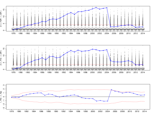
Figure 1: Results of likelihood ratio tests for nested and non-nested models. The points denote the value of the statistic $2\mathcal{R}$ or $\mathcal{R}$ (depending on the test) and the dashed lines show the critical value of the corresponding test (at level 0.05). For the nested case, boxplots show the distribution of $2\mathcal{R}$ for 10000 simulations of the power-law null hypothesis, from which the critical value is computed. The abscissa corresponds to the ending point of a time window starting always in 1 Jan 1977. Note that the year is considered a continuous variable (not a categorical variable), so, the time window ending on 31 Dec 2004 takes value $2004.99\dots\simeq 2005$. (a) Tap distribution versus power law. (b) Truncated gamma versus power law. (c) Truncated gamma versus Tap (non-nested case).

When we compare the power-law fit with the truncated gamma, using the same test, for the same data, the results are more significant, see Fig. 1(b). The situation previous to 2004 is the same, with an extremely poor performance of the power law; but after 2004, despite a big jump again in the value of the likelihood ratio, the power law continues as being non-acceptable, at the 0.05 level. It is only after the great Tohoku earthquake of 2011 that the $p-$value of the test enters into the acceptance region, but keeping values not far from the 0.05 limit. From here we conclude that, in order to find an alternative to the power-law distribution, the truncated gamma distribution is a better option than the Tap distribution, as it is more clearly distinguishable from the power law (for this particular data). Nevertheless, a comparison between these two distributions (Tap and TrG) seems pertinent.

When the models are not nested, as it happens if we want a direct comparison between the Tap and the TrG distributions, the procedure we use is the likelihood ratio test of Vuong for non-nested models Vuong ; Clauset . In this case the critical values depend on the sample size, $N$, turning out to be that, when $N$ is large, $\mathcal{R}$ is normally distributed with standard deviation $s\sqrt{N}$, where $s$ denotes the standard deviation of the set

$$\{\ln f_{trg}(M_{i};\hat{\beta}_{trg},\hat{\theta}_{trg})-\ln f_{tap}(M_{i};\hat{\beta}_{tap},\hat{\theta}_{tap})\}$$

for $i=1,\dots,N$ and $\mathcal{R}=l_{trg}-l_{tap}$. Then, we accept that there exists a significant difference between the models if

$$|\mathcal{R}|>\>1.96s\sqrt{N}$$ (3)

at a level of risk equal to 0.05, with the model with larger log-likelihood being the preferred one. The critical value of the test arises because the null hypothesis is that the mean value of $\mathcal{R}$ is zero (i.e., both models are equally close to the true distribution). Note that the alternative hypothesis corresponds to accept that the difference between the fit provided by the models is significant. As the number of parameters is the same for the Tap and TrG models, their log-likelihood-ratio coincides with the difference in BIC or AIC, but, as mentioned above, the LR test incorporates a statistical test which specifies the distribution of the statistic under consideration.

Figure 1(c) shows the evolution of the log-likelihood-ratio between the two models, for different time windows (starting always in 1977), together with the critical region of the test given by the Eq. (3). One can see how the fits provided by the Tap and TrG distributions do not exhibit significant difference, although the TrG provides, in general, slightly higher likelihoods. After the mega-event in 2004 the performance of the TrG fit improves, approaching the limit of significance. This reinforces our conclusion that the TrG distribution is preferred in front of the Tap and power-law distributions.

In order to gain further insight, we simulate random samples following the truncated gamma distribution, with the parameters $\hat{\beta}_{trg}$ and $\hat{\theta}_{trg}$ obtained from ML estimation of the complete dataset (Table 1), with the same truncation parameter $a$ and number of points ($N=6150$) also. To avoid that the conclusions depend on the time correlation of magnitudes, we reshuffle the simulated data in such a way that the occurrence of the order statistics is the same as for the empirical data; in other words, the largest simulated event is assigned to take place at the time of the 2011 Tohoku earthquake (the largest of the CMT catalog Bell_Naylor_Main ), the second largest at the time of the 2004 Sumatra event, and so on. In this way, we model earthquake seismic moments as arising from a gamma distribution with fixed parameters and with occurrence times given by the empirical times and with the same seismic moment correlations as the empirical data, approximately.

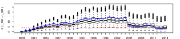
Figure 2: Comparison of the empirical log-likelihood-ratios between the TrG and power law with those of 1000 simulations of the TrG distribution, using the final parameters of Table 1 (i.e., $\beta=0.681$ and $m_{c}=9.15$). Simulated seismic moments are reshuffled as explained in the text to make the comparison possible. Simulation results are displayed using boxplots, representing the three quartiles of the distribution of $2\mathcal{R}$.

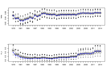
Figure 3: Comparison of the values of the estimated parameters of the TrG distribution, $\hat{\beta}_{trg}$ and $\hat{m}_{c\,trg}$, for the empirical data and for 1000 simulations of the TrG distribution, using the final parameters of Table 1. Simulated seismic moments are reshuffled as explained in the text. The different stability of both parameters is apparent.

We simulate 1000 datasets with $N=6150$ each. The results, displayed in Fig. 2, show that the behavior of the empirical data is not atypical in comparison with this gamma modeling. In nearly all time windows the empirical data lies in between the first and third quartile of the simulated data, although before 2004 the empirical values are close to the third quartile whereas after 2004 they lay just below the median. This leads us to compute the statistics of the jump in the log-likelihood-ratio between 2004 and 2005. The estimated probability of having a jump larger than the empirical value is around 4.5 %, which is not far from what one could accept from the gamma modeling explained above. Thus, a TrG distribution, with fixed parameters, is able to reproduce the empirical findings, if the peculiar time ordering of magnitude of the real events is taken into account. Notice also that, although the simulated data come from a TrG distribution, they are not distinguishable from a power law for about half of the simulations of the last time windows, as the critical region is close to the median indicated by the boxplots.

We can also compare the evolution of the estimated parameters for the empiral dataset and for the reshuffled TrG simulations, with a good agreement again, see Fig. 3. There, it is clear that although the exponent $\beta$ reaches very stable values relatively soon, the scale parameter $\theta$ (equivalent to $m_{c}$) is largely unstable, and the occurrence of the biggest events makes its value increase.

As a complementary control we invert the situation, simulating 1000 syntetic power-law datasets with $\beta=0.685$ (Table 1), $a=5.3\cdot 10^{17}$ N$\cdot$m, and $N=6150$, for which the same time reshuffling is perfomed, in such a way that the order of the order statistics is the same. In this case, the results of the simulations lead to much smaller values of the log-ratio, for which the power-law distribution cannot be rejected (as expected), in contrast with the empirical data, see Fig. 4.

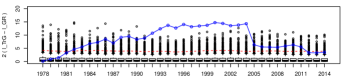
Figure 4: As Fig. 2, but simulating a power law with parameter $\beta=0.685$ (Table 1) instead of a TrG distribution. The reshuffling is also as in Fig. 2, as explained in the text. The simulations cannot explain the large empirical values of the log-likelihood-ratio.

In summary, the truncated gamma distribution represents the best alternative to model global shallow earthquake seismic moments, in comparison with the tapered GR distribution and the power law. The preponderance of the gamma model is maintained after the occurrence of the mega-earthquakes taking place from 2004 and it is only after the 2011 Tohoku earthquake that it is difficult to decide between power law and TrG. We have verified that these results are qualitatively similar if we restrict our study to subduction zones, as defined by the Flinn-Engdahl’s regionalization Kagan_pageoph99 , with the main difference that the values of $l_{trg}-l_{pl}$ become somewhat smaller and therefore the power-law hypothesis cannot be rejected after the Tohoku earthquake.

In order to reproduce the time evolution of the statistical results it suffices that independent gamma seismic moments, with fixed parameters, are reshuffled so that the peculiar empirical time correlations of magnitudes are maintained. So, although the scale parameter $\theta$ is not stabilized, and the occurrence or not of more mega-earthquakes could significantly change its value Zoller_grl , the current value is enough to explain the available data. It would be very interesting to investigate if the high values of the likelihood ratio attained before the 2004 Sumatra event could be employed to detect the end of periods of low global seismic activity. Certainly, more data would be necessary for that purpose Zoller_grl .

As an extra argument in favor of the truncated gamma distribution in front of the tapered GR, we can bring not a statistical evidence but physical plausibility; indeed, the former distribution can be justified as coming from a branching process that is slightly below its critical point Christensen_Moloney ; Corral_FontClos . Further reasons that may support the truncated gamma are that this arises (i) as the maximum entropy outcome under the constrains of fixed (arithmetic) mean and fixed geometric mean of the seismic moment Main_information ; (ii) as the closest to the power law, in terms of the Kullback-Leibler “distance”, when the mean seismic moment is fixed Sornette_Sornette_bssa ; and (iii) as a stable distribution under a fragmentation process with a power-law transition rate Sornette_Sornette_bssa .

We are grateful to J. del Castillo, Y. Y. Kagan, I. G. Main, and M. Naylor for their feedback. Research expenses were founded by projects FIS2012-31324 and MTM2012-31118 from Spanish MINECO, 2014SGR-1307 from AGAUR, and the Collaborative Mathematics Project from La Caixa Foundation.

References

- (1) T. Utsu. Representation and analysis of earthquake size distribution: a historical review and some new approaches. Pure Appl. Geophys., 155:509–535, 1999.
- (2) B. D. Malamud. Tails of natural hazards. Phys. World, 17 (8):31–35, 2004.
- (3) P. Bak. How Nature Works: The Science of Self-Organized Criticality. Copernicus, New York, 1996.
- (4) L. Knopoff and Y. Kagan. Analysis of the theory of extremes as applied to earthquake problems. J. Geophys. Res., 82:5647–5657, 1977.
- (5) A. Corral. Scaling and universality in the dynamics of seismic occurrence and beyond. In A. Carpinteri and G. Lacidogna, editors, Acoustic Emission and Critical Phenomena, pages 225–244. Taylor and Francis, London, 2008.
- (6) Y. Y. Kagan. Universality of the seismic moment-frequency relation. Pure Appl. Geophys., 155:537–573, 1999.
- (7) Y. Y. Kagan. Seismic moment distribution revisited: I. statistical results. Geophys. J. Int., 148:520–541, 2002.
- (8) A. Deluca and A. Corral. Fitting and goodness-of-fit test of non-truncated and truncated power-law distributions. Acta Geophys., 61:1351–1394, 2013.
- (9) Y. Y. Kagan. Earthquakes: Models, Statistics, Testable Forecasts. Wiley, 2014.
- (10) D. Vere-Jones. A branching model for crack propagation. Pure Appl. Geophys., 114:711–725, 1976.
- (11) I. Main. Statistical physics, seismogenesis, and seismic hazard. Rev. Geophys., 34:433–462, 1996.
- (12) G. Zöller. Convergence of the frequency-magnitude distribution of global earthquakes: Maybe in 200 years. Geophys. Res. Lett., 40:3873–3877, 2013.
- (13) D. Vere-Jones, R. Robinson, and W. Yang. Remarks on the accelerated moment release model: problems of model formulation, simulation and estimation. Geophys. J. Int., 144(3):517–531, 2001.
- (14) H. Kanamori. The energy release in great earthquakes. J. Geophys. Res., 82(20):2981–2987, 1977.
- (15) H. Kanamori and E. E. Brodsky. The physics of earthquakes. Rep. Prog. Phys., 67:1429–1496, 2004.
- (16) G. Ekstrom, M. Nettles, and A.M. Dziewonski. The global CMT project 2004-2010: Centroid-moment tensors for 13,017 earthquakes. Phys. Earth Planet. Int., 200-201:1–9, 2012.
- (17) C. Godano and F. Pingue. Is the seismic moment-frequency relation universal? Geophys. J. Int., 142:193–198, 2000.
- (18) Y. Y. Kagan. Earthquake size distribution: Power-law with exponent ? Tectonophys., 490:103–114, 2010.
- (19) T. Lay. Why giant earthquakes keep catching us out. Nature, 483:149–150, 2012.
- (20) I. G. Main, L. Li, J. McCloskey, and M. Naylor. Effect of the Sumatran mega-earthquake on the global magnitude cut-off and event rate. Nature Geosci., 1:142, 2008.
- (21) A. F. Bell, M. Naylor, and I. G. Main. Convergence of the frequency-size distribution of global earthquakes. Geophys. Res. Lett., 40:2585–2589, 2013.
- (22) E. L. Geist and T. Parsons. Undersampling power-law size distributions: effect on the assessment of extreme natural hazards. Nat. Hazards, 72:565–595, 2014.
- (23) Y. Pawitan. In All Likelihood: Statistical Modelling and Inference Using Likelihood. Oxford UP, Oxford, 2001.
- (24) G. Casella and R. L. Berger. Statistical Inference. Duxbury, Pacific Grove CA, 2nd edition, 2002.
- (25) NIST Digital Library of Mathematical Functions. 2014. http://dlmf.nist.gov/8.7#E3.
- (26) P. McCullagh and D. R. Cox. Invariants and likelihood ratio statistics. Ann. Statist., 14(4):1419–1430, 1986.
- (27) S. G. Self and K.-Y. Liang. Asymptotic properties of maximum likelihood estimators and likelihood ratio tests under nonstandard conditions. J. Am. Stat. Assoc., 82:605–610, 1987.
- (28) C. J. Geyer. On the asymptotics of constrained -estimation. 22(4):1993–2010, 1994.
- (29) Y. Y. Kagan. Why does theoretical physics fail to explain and predict earthquake occurrence? In P. Bhattacharyya and B. K. Chakrabarti, editors, Modelling Critical and Catastrophic Phenomena in Geoscience, Lecture Notes in Physics, 705, pages 303–359. Springer, Berlin, 2006.
- (30) Y. Y. Kagan and F. Schoenberg. Estimation of the upper cutoff parameter for the tapered Pareto distribution. J. Appl. Probab., 38A:158–175, 2001.
- (31) Q. H. Vuong. Likelihood ratio tests for model selection and non-nested hypotheses. Econometrica, 57(2):307–33, 1989.
- (32) A. Clauset, C. R. Shalizi, and M. E. J. Newman. Power-law distributions in empirical data. SIAM Rev., 51:661–703, 2009.
- (33) K. Christensen and N. R. Moloney. Complexity and Criticality. Imperial College Press, London, 2005.
- (34) A. Corral and F. Font-Clos. Criticality and self-organization in branching processes: application to natural hazards. In M. Aschwanden, editor, Self-Organized Criticality Systems, pages 183–228. Open Academic Press, Berlin, 2013.
- (35) I. G. Main and P. W. Burton. Information theory and the earthquake frequency-magnitude distribution. Bull. Seismol. Soc. Am., 74(4):1409–1426, 1984.
- (36) D. Sornette and A. Sornette. General theory of the modified Gutenberg-Richter law for large seismic moments. Bull. Seismol. Soc. Am., 89(4):1121–1130, 1999.