Abstract

Signature change at high density has been obtained as a possible consequence of deformed space-time structures in models of loop quantum gravity. This article provides a conceptual discussion of implications for cosmological scenarios, based on an application of mathematical results for mixed-type partial differential equations (the Tricomi problem). While the effective equations from which signature change has been derived are shown to be locally regular and therefore reliable, the underlying theory of loop quantum gravity may face several global problems in its semiclassical solutions.

1 Introduction

Anomaly-free effective models of loop quantum gravity, derived for spherically symmetric configurations [1, 2] and cosmological perturbations at high density [3, 4], have revealed an unexpected phenomenon: At large curvature, signature change appears to be a generic feature of quantum space-time geometry as provided by this theory [5]. Not only the general phenomenon but also the specific form of signature change seems to be universal in these models, giving further support of the genericness of the effect. For the typical form of “holonomy modifications” used widely in models of loop quantum gravity, the speed of physical modes differs from the classical speed of light by a factor of $\beta(h,K):=\alpha(h)\cos(2\delta K)$ where $\alpha(h)>0$ is a function of the spatial geometry (the metric $h$), $\delta$ is a quantization parameter often assumed to be related to the Planck length, and $K$ is a measure for extrinsic curvature (or the Hubble parameter in cosmological models). For large curvature $K>\pi/(4\delta)$, the speed is negative and commonly hyperbolic mode equations turn elliptic, which in these models are of the form

$$\frac{\partial^{2}\phi}{\partial t^{2}}-\frac{\beta(h,K)}{a^{2}}\Delta\phi=S[\phi]$$ (1)

with source and lower-derivative terms $S[\phi]$. All modes $\phi$, gravitational as well as matter, are affected in the same way.

The overall picture shows some relationships with other approaches to quantum cosmology, mainly the no-boundary proposal of Hartle and Hawking [6], and with other physical phenomena such as transonic flow or phases of nano-wires. Related mathematical questions have been studied in the mathematical literature since the 1930s, following seminal work by Tricomi [7]. Nevertheless, as a basis of effective space-time models, equations of the form (1) and the phenomenon of signature change show several new and surprising features. In this article, we give a general presentation of implications in cosmology.

Section 2 gives a definition of signature change in the absence of a classical space-time metric, and contains a brief comparison with classical models of signature change. (A review of the formal origin and gauge independence of equation (1) and signature change can be found in App. A.) Section 3 provides several related examples in different areas of physics together with the appropriate mathematical formulation in terms of well-posed partial differential equations. Section 4 applies these results to gravitational questions, compares the pictures based on effective equations with wave-function methods, draws cosmological implications, and ends with cautious notes on global issues.

2 Definitions

Despite first appearance, the wave equation (1) is covariant under a deformed algebra replacing classical coordinate or Poincaré transformations. The corresponding quantum space-time structure is not Riemannian, but has a well-defined canonical formulation using hypersurface deformations, as reviewed briefly in the appendix.

A Riemannian manifold has a covariant metric tensor which transforms by $g_{a^{\prime}b^{\prime}}=(\partial x^{a}/\partial x^{a}{}^{\prime})(\partial x^{b}/\partial x^{b}{}^{\prime})g_{ab}$ when coordinates are changed on the manifold. Accordingly, the line element ${\rm d}s^{2}=g_{ab}{\rm d}x^{a}{\rm d}x^{b}=g_{a^{\prime}b^{\prime}}{\rm d}x^{a^{\prime}}{\rm d}x^{b^{\prime}}$ is invariant. Covariance under coordinate transformations (of solutions to the field equations) is canonically represented as gauge-invariance under hypersurface deformations in space-time [8]. Since the latter, along with Poincaré transformations, are modified in the effective space-time structures we are considering, they can no longer correspond to coordinate transformations. As a consequence, the effective “metric” does not give rise to an invariant line element. Instead of using metric-space notions such as geodesics and invariant scalar products of 4-vectors, in order to extract predictions there is only the possibility of computing canonical observables invariant under the modified gauge transformations. In this way, one still has access to all observable information. However, the lack of a metric structure implies that many of the convenient and well-known techniques of evaluating solutions of general relativity are no longer available.

Although there is no standard notion of geodesics and light rays or null lines, it remains straightforward to associate a causal structure to the modified space-time structure underlying (1), as long as $\beta>0$. Instead of computing null lines for a metric, we just use characteristics of the wave equation (1), for instance for gravitational waves to be specific. (In the presence of inverse-triad corrections, scalar modes may propagate at speeds different from tensor modes [9, 4].) A characteristic is then a hypersurface which at any point is normal to a vector $k^{a}$ satisfying $(k^{t})^{2}-\beta|\vec{k}|^{2}=0$. With these characteristics instead of null lines, we can define light cones, a causal structure, and derived notions such as Penrose diagrams.

Characteristics exist as long as $\beta>0$. For holonomy modifications, $\beta$ changes sign at high density, and the characteristic equation no longer has non-trivial solutions $k^{a}\not=0$. As a consequence, (1) does not provide a causal structure in such a regime. Since the same condition of $\beta<0$ makes the mode equation (1) turn elliptic, we call this regime “Euclidean,” while for $\beta>0$ we call it “Lorentzian.” In this way, we generalize the two standard discrete choices of signature to a continuous range of values taken by $\beta$ as it varies from the classical limit $\beta=1$ at low curvature to a negative value at high curvature. Unless $\beta=\pm 1$, the canonical fields from which (1) is derived do not provide a classical notion of Lorentzian space-time or 4-dimensional Euclidean space. But the most important properties regarding physical consequences, including the existence of a causal structure and the type of initial or boundary value problem required for reliable solutions, only depend on the sign of $\beta$ rather than its precise value. For this reason, we still speak of Euclidean or Lorentzian signature even if we have neither Euclidean nor Lorentzian space(-time).

Signature change has been studied in quite some detail in classical general relativity ($\beta=1$); see for instance [10]. However, such models are crucially different from what is considered here, in that they have $\beta{\rm sgn}(\det h_{ab})$ (or $\beta{\rm sgn}N^{2}$) changing discontinuously. As a consequence, in classical models the transition from Euclidean to Lorentzian signature is always singular, which is not the case in our effective models. (Note that for this reason signature change in the model of [11] is not analogous to deformed space-time structures.) The subtleties and controversies related to the distributional nature of solutions with classical signature change, discussed for instance in [12, 13, 14, 15, 16, 17, 18], do not play a role in our context. (The models we study could be considered as a version of dynamical signature change as anticipated in the conclusions of [19].)

It is necessary to consider inhomogeneity in order to see modified space-time structures in which modes obey (1). In particular the phenomenon of signature change, which is the main topic of this article and is realized because $\beta$ may change sign, can only be seen in inhomogeneous models: it is manifested by the relative sign in space and time derivatives in field equations. However, signature change (or a modified space-time structure) is not a consequence of inhomogeneity, which in the perturbative context would be dubious [20]. The origin of signature change lies in the modification that one makes in the classical dynamics if one quantizes the theory following loop quantum gravity, which provides operators for holonomies (exponentiated and integrated connections) instead of ordinary connection components. This modification appears already in the background dynamics of a homogeneous minisuperspace model, but in this context one does not notice signature change because all spatial derivatives vanish. Perturbative inhomogeneity then makes the effect visible. Still, inhomogeneity or perturbation theory is not the origin of signature change, which is easy to see by the following two arguments: First, signature change persists in a perturbative field equation no matter how small the inhomogeneity is, as long as it is non-zero. The coefficients of space and time derivatives in (1) depend on background quantities, and for $\beta<0$ they have the same sign for all values of inhomogeneity. Secondly, the same form of signature change appears in spherically symmetric models in which inhomogeneity need not be treated perturbatively.

3 Related effects

In the explicit form as provided by models of loop quantum gravity, signature change is a new effect. But it has precursors in physics as well as mathematics. Besides the examples discussed in details below, the case of helically symmetric binary systems [21] is worth mentioning. The configuration is described by partial differential equations which change signature along a spacelike direction (far from the center), rather than a timelike one as in our cosmological models.

3.1 Hartle–Hawking wave function

A Lorentzian space-time cannot be closed off at a finite time without a boundary. As proposed in [6], however, one may postulate that quantum gravity gives rise to a modified space-time structure that allows a transition to Euclidean 4-dimensional space. A Euclidean cap can then be attached to a space-time manifold which becomes Lorentzian at low curvature. In [6] and the literature based on it, this scenario has been used mainly to specify the high-density asymptotics of wave functions satisfying the Wheeler–DeWitt equation of homogeneous models.

The scenario suggested by effective constraints in models of loop quantum gravity can be seen as a concrete realization of the quantum-gravity effects that may give rise to signature change. The condition that extrinsic curvature vanish at the interface between Euclidean and Lorentzian parts of semiclassical solutions [22] is then replaced by $\beta(h,K)=0$. Nevertheless, it is not guaranteed that the same consequences are implied for wave functions, not the least because the possibility of signature change relies on a quantum-geometry effect (based on the use of holonomies in loop quantum gravity) which turns the Wheeler–DeWitt equation into a difference equation [23, 24]. The minisuperspace discreteness implied by this difference equation is relevant especially at high density, that is in the Euclidean phase where asymptotic properties are discussed according to [6]. Qualitatively different conclusions for wave functions could then be reached, so that it is not clear whether the close relationship in the space-time picture of [6] with the models discussed here implies a similar relationship in predictions. Specific details of wave functions might well be closer to [25] than to [6]. We leave this question open in the present article, in which we are concerned mainly with effective equations.

3.2 Analog condensed-matter models

In addition to related cosmological models in terms of space-time properties, there are rather different physical phenomena which give rise to mathematical descriptions similar to (1). The main examples known to us are transonic flow and hyperbolic metamaterials [26]. Especially the latter phenomenon provides an interesting analog picture of the cosmological effects.

An example of a hyperbolic metamaterial is given by an array of parallel conducting nano-wires immersed in a dielectric medium. Such a material behaves as a conductor in the direction parallel to the nano-wires while in the normal one it exhibits dielectric properties [27]. Choosing the $z$-axis to be parallel to the nano-wires, the wave equation for the component $E^{z}=:\phi$ of the electromagnetic field can be written as [27]

$$\frac{\partial^{2}\phi}{\partial t^{2}}-\frac{1}{\epsilon_{\bot}}\frac{\partial^{2}\phi}{\partial z^{2}}-\frac{1}{\epsilon_{||}}\left(\frac{\partial^{2}\phi}{\partial x^{2}}+\frac{\partial^{2}\phi}{\partial y^{2}}\right)=0\,.$$ (2)

For the “wired” metamaterials the electric permittivity is $\epsilon_{||}>0$, as for the standard dielectric medium. However, because the metamaterial is conducting in the $z$-direction, $\epsilon_{\bot}$ will be negative in a sufficiently low frequency range. In particular, for the Drude theory of a conducting medium

$$\epsilon_{\bot}=1-\frac{\omega^{2}_{\rm P}}{\omega^{2}}\,,$$ (3)

where $\omega_{\rm P}$ is the plasma frequency dependent on the geometry and composition of the metamaterial. At low frequencies ($\omega<\omega_{\rm P}$), $\epsilon_{\bot}>0$ and the spatial part of equation (2) is elliptic. However, for $\omega>\omega_{\rm P}$, we have $\epsilon_{\bot}<0$ and the sign in front of the second derivative with respect to $z$ changes. The spatial Laplace operator becomes hyperbolic, with the $z$-component playing a role of the second time variable. The dispersion relation

$$\omega^{2}-\frac{k_{z}^{2}}{\epsilon_{\bot}}-\frac{k^{2}_{||}}{\epsilon_{||}}=0\,,$$ (4)

where $k^{2}_{||}:=k_{x}^{2}+k_{y}^{2}$, for fixed $\omega$ is in this regime no longer represented by ellipsoids but hyperboloids. In consequence, the $k$-space undergoes a topology change.

Passing between the elliptic and hyperbolic regions is not only a matter of frequency dependence. For a fixed (sufficiently low) frequency, the transition between the different signs of $\epsilon_{\bot}$ can be induced by a rearrangement in the structural form of the “wired” metamaterial. In particular, melting of the nano-wires to the liquid phase (associated with a first-order phase transition) has been observed experimentally. During the process the value of $\epsilon_{\bot}$ smoothly changes its sign (from negative to positive) with increasing temperature.

Alternatively one can imagine the transition to be of the second order. This idea in the context of signature change due to holonomy corrections has been discussed in [29, 30, 31]. Let us imagine that the nanowires are immersed in a dielectric fluid, having an ability to rotate. Furthermore, let us introduce magnetic dipole-dipole type interactions between the wires by attributing magnetic moments to them. Then, in the high temperature unordered phase, with all nano-wires pointing in random directions, there is hardly any electric conductivity. But when the phase changes to an ordered one (lowering the temperature), a significant electric current starts flowing, just as time starts flowing in our universe models when the density is small enough to trigger signature change to Lorentzian space-time.

In the gravitational case, the process can be modelled by a bi-metric gravity theory, where the effective metric experienced by the fields is

$$g_{\mu\nu}=\delta_{\mu\nu}-2\chi_{\mu}\chi_{\nu}\,.$$ (5)

The metric may be viewed as a 4-dimensional analog of the inverse of the electric permittivity tensor $\epsilon_{ij}$. The $\chi_{\mu}$ is an effective mean field having the interpretation of an order parameter, defined such that in the unordered phase $|\vec{\chi}|=0$ (here $|\vec{\chi}|=\sqrt{\delta^{\mu\nu}\chi_{\mu}\chi_{\nu}}$). In this case the fields experience the Euclidean metric $g_{\mu\nu}=\delta_{\mu\nu}$. In the fully ordered phase $|\vec{\chi}|=1$, the Lorentzian signature emerges in a spontaneously chosen direction in the 4-dimensional space.

In order to describe the transition from the unordered to the ordered state more quantitatively let us postulate the following form of the free energy for a model with a test field $\phi$:

$$F=\int{\rm d}V\underbrace{\left(\delta^{\mu\nu}+\frac{2\chi^{\mu}\chi^{\nu}}{1-2|\vec{\chi}|^{2}}\right)}_{g^{\mu\nu}}\partial_{\mu}\phi\partial_{\nu}\phi+\underbrace{C\left[\left(\frac{\rho}{\rho_{\rm QG}}-1\right)|\vec{\chi}|^{2}+\frac{1}{2}|\vec{\chi}|^{4}\right]}_{V(\chi^{\mu},\rho)}\,,$$

where $C$ is a constant. Because of the $\chi^{\mu}\chi^{\nu}\partial_{\mu}\phi\partial_{\nu}\phi$ contribution to the kinetic term, $F$ is not SO(4)-invariant in the internal indices of $\chi^{\mu}$. The explicit symmetry-breaking term can be treated perturbatively. Then, equilibrium corresponds to a minimum of the SO(4)-invariant potential $V(\chi^{\mu},\rho)$. In order to model signature change in loop quantum cosmology with maximum energy density $\rho_{\rm QG}$, the parameters of the potential are fixed such that at energy densities $\rho>\rho_{\rm QG}$ the vacuum state maintains the SO(4) symmetry — the order parameter is $|\vec{\chi}|=0$. For $\rho\leq\rho_{\rm QG}$, we choose the potential so that its minimum is located at $|\vec{\chi}|=\sqrt{1-\rho/\rho_{\rm QG}}$, with some spontaneously chosen direction in the 4-dimensional configuration space of the order parameter. Without loss of generality, we may assume $\vec{\chi}$ to point in the $0$-direction ($\chi_{0}=|\vec{\chi}|$ and $\chi_{i}=0$ for $i=1,2,3$); thus, $g_{00}=1-2\chi_{0}\chi_{0}=-1+2\rho/\rho_{\rm QG}=-\beta$ and $g_{ii}=1$. The corresponding wave equation for the test field is

$$-\frac{1}{\beta}\frac{\partial^{2}}{\partial t^{2}}\phi+\Delta\phi=0\,,$$ (6)

which is of the form (1) with $\beta=1-2\rho/\rho_{\rm QG}$ as in models of loop quantum cosmology. At $|\vec{\chi}|=0$ ($\beta=1$) the equation exhibits the $R^{4}\rtimes{\rm SO}(4)$ symmetry while in the fully ordered state $|\vec{\chi}|=1$ ($\beta=-1$) the $R^{1,3}\rtimes{\rm SO}(1,3)$ Poincaré symmetry is satisfied.

It is worth stressing that the presented model relating signature change with the spontaneous symmetry braking of $SO(4)$ has no support from more fundamental considerations at the moment. Therefore, its physical validity requires further studies. In particular, a possible relation of the order parameter $\chi_{\mu}$ with the elementary degrees of freedom of loop quantum gravity remains unclear. Nevertheless, the model presents an interesting example because of its formal resemblance to signature change in loop quantum cosmology. There is, however, an important conceptual difference: while analog models of signature change are fully well-defined and even have some observable properties, quantum-cosmology effects on space-time itself (rather than matter fields in space-time) may be subject to several global problems on which we will comment in Sec. 4.2.6.

3.3 Mixed-type characteristic problem and Tricomi equation

Partial differential equations of mixed type have been studied in the mathematics literature since the 1930s, beginning with the Tricomi problem for the differential equation

$$\frac{\partial^{2}u}{\partial y^{2}}+y\frac{\partial^{2}u}{\partial x^{2}}=0$$ (7)

in the $(x,y)$-plane. This type of equation can be seen as an approximation to our equation (1) around one of the finite boundaries of the elliptic regime, where $\beta=0$. Here, we recall relevant features of a suitable characteristic problem [7, 32].

Let us suppose that we would like to solve equation (7) in a domain $\Omega=\Omega_{1}\cup\Omega_{2}$, where $\Omega_{1}$ and $\Omega_{2}$ are elliptic and hyperbolic domains, respectively. For the Tricomi problem, the sub-domain $\Omega_{2}$ cannot be chosen in an arbitrary manner. Namely, the boundary $\partial\Omega_{2}$ is determined by characteristics of (7) attached to the endpoints of $\partial\Omega_{1}$ at the interface between the hyperbolic and elliptic regions; see Fig. 1. The characteristics in the hyperbolic region are determined by the characteristic equation to (7): $({\rm d}x)^{2}+y({\rm d}y)^{2}=0$. This equation has two families of solutions with a different sign, enabling us to introduce the characteristic coordinates

$$\xi:=x+\frac{2}{3}(-y)^{3/2}\,,$$ (8)

$$\eta:=x-\frac{2}{3}(-y)^{3/2}\,.$$ (9)

(We have $y<0$ in the hyperbolic region.)

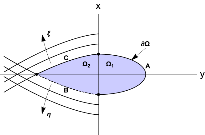
Figure 1: Graphical representation of the characteristic problem from the mixed-type Tricomi equation. Solutions to a partial differential equation (7) (hyperbolic for $y<0$ and elliptic for $y>0$) exist uniquely and stably in the shaded region $\Omega_{1}\cup\Omega_{2}$, provided boundary data are imposed on one characteristic $C$ of the hyperbolic region together with a curve $A$ in the elliptic region. Characteristic coordinates (11) are indicated by $\xi$ and $\eta$.

Solutions to the Tricomi equation (7) are unique and stable if adequate boundary conditions are imposed. Applying the notation from Fig. 1, they are as follows: in region $\Omega_{1}$, the value of $u$ has to be specified at the boundary curve $A$, while in region $\Omega_{2}$ the value of $u$ at the characteristic curve $C$ has to be given. The value of $u|_{B}$ is a result of fixing the boundary condition $u|_{C\cup A}$.

The reason why the boundary condition in the hyperbolic region is imposed on the characteristic curve becomes clear by analyzing the case of the standard wave equation with one spatial dimension:

$$\frac{\partial^{2}u}{\partial y^{2}}-\frac{\partial^{2}u}{\partial x^{2}}=0\,.$$ (10)

The corresponding characteristic equation $({\rm d}x)^{2}-({\rm d}y)^{2}=0$ has solutions $x\pm y=C$, which allow us to introduce the characteristic (light cone) variables

$$\xi:=x+y\,,$$ (11)

$$\eta:=x-y\,.$$ (12)

In terms of these variables the wave equation (10) reduces to the canonical form

$$\frac{\partial^{2}u}{\partial\xi\partial\eta}=0\,,$$ (13)

with general solution $u=f(\xi)+g(\eta)$. An important observation is that an initial-value problem (Cauchy problem) in the variables $(x,y)$ translates into the boundary-value problem in the characteristic variables $(\xi,\eta)$. In particular, the Cauchy-problem initial condition $u|_{y=0}$ and $\left.\partial u/\partial y\right|_{y=0}$ translates into the Dirichlet boundary condition at the light cone $u|_{\xi=0}$ and $u|_{\eta=0}$.

Using characteristics, it is therefore easier to combine hyperbolic and elliptic regimes. In the case of the Tricomi equation, the boundary conditions in the elliptic domain have to be smoothly extended into the hyperbolic sector. This requires the introduction of characteristic variables in the hyperbolic sector, imposing boundary conditions at either $\xi=$ constant or $\eta=$ constant (but not both).

4 Cosmology

Signature change plays an important role in cosmological scenarios. In practical terms, one of the most important consequences is the presence of instabilities, as indicated formally by an imaginary speed of sound in mode equations. The same kind of instability plays a role in the mathematical discussion of equations of the form (1): One of the conditions for a well-posed initial/boundary-value problem of a partial differential equation is the stable dependence of solutions on the chosen data, in addition to the conditions that a solution exist and be unique for given data.

4.1 Instability

Stability is easily violated when one attempts to use an initial-value problem for an elliptic equation. For instance, Fourier modes of solutions to the standard wave equation would not oscillate as per $\exp(\pm i\omega t)$ but change exponentially according to $\exp(\pm\omega t)$. The exponentially growing mode implies instability in the sense that solutions, if they exist and are perhaps unique, depend sensitively on the initial values. Choosing a boundary-value problem in $t$ (as well as spatial directions), on the other hand, ties down the solution at both ends of the $t$-range, so that the growing branch is sufficiently restricted for solutions to be stable.

Signature change implies instability of initial-value problems, but it is stronger in two respects. First, signature change affects all modes (of matter or gravity) equally, which all become unstable at the same “time.” It is therefore a space-time effect, rather than an exotic matter phenomenon. Secondly, it can be seen in space-time symmetries such as hypersurface deformations or the Poincaré algebra. None of these effects happen in known cases of instabilities in matter theories or higher-curvature gravitational actions, such as [33]. Signature change is therefore more fundamental than other phenomena hat might imply instability. An important property is the fact that the theory does not provide any causal structure whatsoever when the signature turns Euclidean.

4.2 Scenarios

When used in cosmological model-building, signature change implies a new and interesting mixture of linear and cyclic models. One of its main consequences can be described as a finite beginning of the universe. In the simplest versions of existing models of loop quantum cosmology, effective equations do not imply divergences at high density but instead extend solutions to a new low-density regime [34]. The main example is a modified Friedmann equation

$$\frac{\sin(\delta\bar{\cal H})^{2}}{\delta^{2}}=\frac{8\pi G}{3}\rho$$ (14)

postulated for spatially flat isotropic models sourced by a free, massless scalar $\phi$. The energy density $\rho$ is therefore of the form $\rho=\frac{1}{2}p_{\phi}^{2}/a^{6}$ with the momentum $p_{\phi}$ of $\phi$ and the scale factor $a$. In (14), $\delta$ is a parameter which approaches $\delta\to 0$ in the classical limit, and whose precise value remains undetermined. (As a parameter motivated by quantum-gravity effects, it is often assumed to be close to the Planck length.) Moreover, $\bar{\cal H}=(2\delta)^{-1}\arcsin(2\delta\dot{a}/a)$ is a modified version of the Hubble parameter. It is straightforward to see that the modified equation (14) implies that the energy density, for fixed $\delta$, is always bounded, $\rho\leq\rho_{\rm QG}:=3/(8\pi G\delta^{2})$. The parameter $\rho_{\rm QG}$ is the maximum kinetic energy density realized at the bounce. There is then a good chance that cosmological singularities may be resolved. Indeed, the quantum model with a free, massless scalar can be solved completely [35], implying that the scale factor

$$a(t)=a_{0}\left(1+24\pi G\rho_{\rm QG}\>t^{2}\right)^{1/6}$$ (15)

never becomes zero. (See also [36].)

Equation (14), although it remains unclear how generically it is realized for the background evolution [37] of general homogeneous models, has suggested a picture in which our expanding universe descends from a preceding collapse phase which produced large but not infinite density at the big bang. However, when modes on such a bouncing background are subject to equations of the form (1), as required for a consistent system of both background variables $(a,\phi)$ and inhomogeneous modes in models of loop quantum gravity, the transition is not deterministic owing to the lack of causal structure at high density. In the cosmological case, the role of $K$ in (1) is played by the modified Hubble parameter $\bar{\cal H}$. With $\beta(\bar{\cal H})\propto\cos(2\delta\bar{\cal H})$, one can easily see that signature change happens when the energy density is half the maximum it can achieve (or half the bounce density of a homogeneous model). Given the solution (15), the mode equation (1) is elliptic for

$$t^{2}<t_{\rm max}^{2}:=\frac{1}{24\pi G\rho_{\rm QG}}\,.$$ (16)

(For $\rho_{\rm QG}$ close to the Planck density, the $t$-range in which the equation is elliptic is close to the Planck time, but it can be significantly longer in models with a scalar potential or strong quantum fluctuations at high density [38].) The high-density regime cannot be accessed causally, and there is no deterministic transition from collapse to expansion. For practical purposes, such a scenario therefore shares some features with the traditional singular big-bang model, in which one must pose initial values just after the singularity. Similarly, one must pose initial values “after” the Euclidean phase of a signature-change scenario. However, the relationship between singular and signature-change models is subtle, as shown by the detailed discussion of suitable data for mixed-type differential equations on which we now embark.

4.2.1 Gravitational waves

To be more specific, let us focus now on the case of gravitational waves with holonomy corrections. In this case, the equation of motion for each component of polarization of the gravitational waves is [39]

$$\frac{\partial^{2}\phi}{\partial t^{2}}+\left(3H-\frac{\dot{\beta}}{\beta}\right)\frac{\partial\phi}{\partial t}-\frac{\beta}{a^{2}}\Delta\phi=0\,,$$ (17)

where $H:=\frac{\dot{a}}{a}$ is the Hubble parameter and the deformation factor is

$$\beta=\cos(2\delta\bar{\cal H})=1-2\frac{\rho}{\rho_{\rm QG}}\,.$$ (18)

Depending on the value of the parameter $\beta$, equation (17) can be either hyperbolic ($\beta>0$), elliptic ($\beta<0$) or parabolic ($\beta=0$). The transition between elliptic and hyperbolic type (associated with signature change) takes place at $\rho=\frac{1}{2}\rho_{\rm QG}$. At this moment, the square of the Hubble factor $H$ reaches its maximal value $H^{2}_{\rm max}=\frac{2}{3}\pi G\rho_{\rm QG}$. For the model with a free scalar field introduced in the previous section, this takes place at $t=\pm t_{\rm max}=\pm(24\pi G\rho_{\rm QG})^{-1/2}$.

Equation (17) is precisely of the form (1) with the source term

$$S[\phi]=-\left(3H-\frac{\dot{\beta}}{\beta}\right)\frac{\partial\phi}{\partial t}\,.$$ (19)

Because generally $\dot{\beta}\neq 0$ at $\beta=0$, signature change is associated with a divergence of the source. The divergence, however, does not lead to pathological behavior at the level of solutions to equation (17) because, as we will see later, it is due to a regular pole, which does not disturb regularity of the solution. In the vicinity of $\beta=0$, equation (17) can be approximated by

$$\frac{\partial^{2}\phi}{\partial t^{2}}+\left(3H-\frac{\dot{\beta}}{\beta}\right)\frac{\partial\phi}{\partial t}\approx 0\,,$$ (20)

which after double integration leads to the solution

$$\phi=c_{1}+c_{2}\int^{t}\frac{\beta(t^{\prime})}{a(t^{\prime})^{3}}dt^{\prime},$$ (21)

where $c_{1}$ and $c_{2}$ are some functions of the spatial variables. Because $\beta$ occurs in the numerator of the integrand, the approximate solution is indeed regular.

Let us now analyze the behavior of equation (17) in the vicinity of the instance of signature change for the model with a free scalar field. Without loss of generality, we perform an expansion around $t=-t_{\rm max}$, for which

$$\left(3H-\frac{\dot{\beta}}{\beta}\right)=\frac{t(t^{2}-5t^{2}_{\rm max})}{t^{4}-t^{4}_{\rm max}}=-\frac{1}{t+t_{\rm max}}-\frac{1}{t_{\rm max}}+\frac{t+t_{\rm max}}{4t^{2}_{\rm max}}+\mathcal{O}\left((t+t_{\rm max})^{2}\right)\,.$$ (22)

(In the first step we have used (15), (16) and (18) in order to write $a(t)=a_{0}(1+t^{2}/t_{\rm max}^{2})^{1/6}$ and $\beta(t)=1-2(1+t^{2}/t_{\rm max}^{2})^{-1}$.) Because $(t+t_{\rm max})\left(3H-\dot{\beta}/\beta\right)=-1+\mathcal{O}\left(t+t_{\rm max}\right)$, the pole at $t=-t_{\rm max}$ is of the regular type. Furthermore

$$\frac{\beta}{a^{2}}=\frac{(t/t_{\rm max})^{2}-1}{(1+(t/t_{\rm max})^{2})^{4/3}}=-\frac{t+t_{\rm max}}{2^{1/3}t_{\rm max}}+\mathcal{O}\left((t+t_{\rm max})^{2}\right)\,,$$ (23)

where we fixed $a_{0}=1$.

Applying the above expansions to the leading order and reducing to the (1+1)-dimensional case, we obtain

$$\frac{\partial^{2}\phi}{\partial t^{2}}-\frac{1}{t+t_{\rm max}}\frac{\partial\phi}{\partial t}+\frac{t+t_{\rm max}}{2^{1/3}t_{\rm max}}\frac{\partial^{2}\phi}{\partial x^{2}}=0\,.$$ (24)

Redefining the time variable to

$$y:=\frac{1}{\left(2^{1/3}t_{\rm max}\right)^{1/3}}(t+t_{\rm max})\,,$$ (25)

equation (24) can be rewritten as

$$\frac{\partial^{2}\phi}{\partial y^{2}}+y\frac{\partial^{2}\phi}{\partial x^{2}}=\frac{1}{y}\frac{\partial\phi}{\partial y}\,.$$ (26)

The left-hand side of this equation is identical to Tricomi’s expression in (7) while the right-hand side can be treated as a source term. Applying the characteristic Tricomi problem to obtain solutions to the equation (26) is therefore justified.

It is worth noting at this point that equation (26) in the vicinity of $y=0$ reduces to

$$\frac{\partial^{2}\phi}{\partial y^{2}}-\frac{1}{y}\frac{\partial\phi}{\partial y}=0\,,$$ (27)

with solution $\phi=c_{1}+c_{2}y^{2}$ (in agreement with (21)). The solution is perfectly regular across the signature change, in contrast to classical signature change. In particular, signature change resulting from the line element ${\rm d}s^{2}=-t{\rm d}t^{2}+{\rm d}x_{a}{\rm d}x^{a}$ has been widely studied in the literature [12, 13, 16]. In this case, the analog of equation (27) is $\frac{\partial^{2}\phi}{\partial y^{2}}-\frac{1}{2y}\frac{\partial\phi}{\partial y}=0$, with the metric signature change at $y=0$. While both forms of the equation look very similar, the extra factor of “2” plays a significant role leading to the non-differentiability of solution at the signature change. For discussion of controversies around this issue as well as some proposals of dealing with the problem we refer to Ref. [16].

Coming back to expression (26), the corresponding equation for the Fourier component $\phi_{k}=(2\pi)^{-1/2}\int{\rm d}ke^{-ikx}\phi(x)$ is

$$\frac{\partial^{2}\phi_{k}}{\partial z^{2}}-\frac{1}{z}\frac{\partial\phi_{k}}{\partial z}-z\phi_{k}=0\,,$$ (28)

where $z:=y|k|^{2/3}$ has been introduced to absorb the wave number $k$. In order to facilitate solving this equation, we observe that by differentiating the Airy equation

$$\frac{{\rm d}^{2}u}{{\rm d}z^{2}}-zu=0\,,$$ (29)

and subsequently substituting for $u$ using again (29), we find an equation

$$\frac{{\rm d}^{3}u}{{\rm d}z^{3}}-\frac{1}{z}\frac{{\rm d}^{2}u}{{\rm d}z^{2}}-z\frac{{\rm d}u}{{\rm d}z}=0$$ (30)

identical to (28) if $\phi_{k}={\rm d}u/{\rm d}z$ for a suitable ($k$-dependent) $u$ solving (29). Solutions to (28) are therefore

$$\phi_{k}=A_{k}{\rm Ai}^{\prime}(z)+B_{k}{\rm Bi}^{\prime}(z)\,,$$ (31)

where ${\rm Ai}^{\prime}(z)$ and ${\rm Bi}^{\prime}(z)$ are the Airy prime functions (derivatives of the Airy functions) and $A_{k}$ and $B_{k}$ are $k$-dependent constants of integration. Because of the reality condition for the field $\phi$ the following relations have to be fulfilled: $A^{*}_{k}=A_{-k}$ and $B^{*}_{k}=B_{-k}$.

As an example, we will now apply the Tricomi boundary conditions to the resulting 2-dimensional solution

$$\phi(y,x)=\int_{-\infty}^{+\infty}\frac{{\rm d}k}{\sqrt{2\pi}}e^{ikx}\left[A_{k}{\rm Ai}^{\prime}\left(y|k|^{2/3}\right)+B_{k}{\rm Bi}^{\prime}\left(y|k|^{2/3}\right)\right]\,.$$ (32)

First, let us choose the contour $A:=\left\{(x,y)\in\mathbb{R}^{2},y=0,-\pi<x<\pi\right\}$ and fix $\phi|_{A}=\cos{x}$. This condition reduces (32) to

$$\phi(y,x)=\cos(x)\left[\frac{1-c_{0}{\rm Bi}^{\prime}(0)}{{\rm Ai}^{\prime}(0)}{\rm Ai}^{\prime}(y)+c_{0}{\rm Bi}^{\prime}(y)\right]\,,$$ (33)

with a parameter $c_{0}\in\mathbb{R}$. Secondly, the form of $A$ implies that:

$$C := \left\{(x,y)\in\mathbb{R}^{2},x=\pi-\frac{2}{3}(-y)^{3/2},-\left(\frac{3\pi}{2}\right)^{2/3}<y<0\right\}\,,$$ (34)

$$B := \left\{(x,y)\in\mathbb{R}^{2},x=-\pi+\frac{2}{3}(-y)^{3/2},-\left(\frac{3\pi}{2}\right)^{2/3}<y<0\right\}\,.$$ (35)

Finally, by choosing

$$\phi|_{C}=\cos\left(\pi-\frac{2}{3}(-y)^{3/2}\right){\rm Ai}^{\prime}(y)/{\rm Ai}^{\prime}(0)$$ (36)

the constant $c_{0}$ is fixed to equal zero, which leads to

$$\phi(y,x)=-3^{1/3}\Gamma(1/3)\cos(x){\rm Ai}^{\prime}(y)\,.$$ (37)

The solution together with the boundary $\partial\Omega=A\cup B\cup C$ is shown in Fig. 2. For all other values of $c_{0}$, the contribution from ${\rm Bi}^{\prime}(y)$ in (33) does not vanish, and therefore the solution is characterized by an exponential growth in the $y>0$ region. Nevertheless, in the domain enclosed by $\partial\Omega=A\cup B\cup C$ the solution remains regular. It is transparent from Fig. 2 that the monotonic solution in the elliptic region ($y>0$) transforms smoothly into the oscillatory solution in the hyperbolic domain ($y<0$), as expected intuitively.

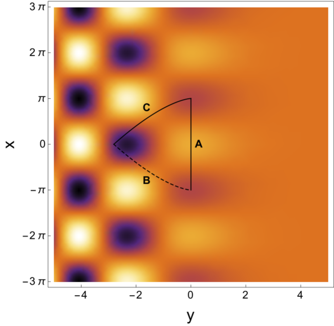
Figure 2: Density plot of the solution (37) together with the boundary $\partial\Omega=A\cup B\cup C$. This special solution is exponentially decreasing for $y>0$, as can be seen by the fading-away of oscillations.

4.2.2 Characteristic problem

We are now in a position to adapt the Tricomi problem to effective space-time models of loop quantum gravity. We begin with a qualitative discussion which also provides heuristic reasons for why the mixed-type initial-boundary value problem must be used.

In a non-singular universe model in which collapse is joined by expansion, one can start with initial values in the collapsing Lorentzian phase in the past and evolve all the way to the boundary with the Euclidean phase (at $t=-t_{\rm max}$ in the solvable model). For a second-order hyperbolic differential equation in this regime, we need to fix initial values $\phi$ and $\phi^{\prime}$, where we denote by $\phi^{\prime}$ the derivative of $\phi$ normal to constant-$t$ hypersurfaces. In this regime, $\phi^{\prime}$ may therefore be considered as the time derivative of $\phi$. When we reach the Euclidean phase, time no longer exists in a causal sense and our coordinate $t$ is one of the four spatial ones. We will continue denoting the $t$-derivative as $\phi^{\prime}$, now strictly in the sense of a normal derivative replacing the time derivative.

Figure 3: Illustration of indeterministic behavior implied by the mixed-type differential equations of signature-change cosmology. The boxed data for a field $\phi$ — the field and its first normal derivative $\phi^{\prime}$ in the past Lorentzian phase as well as the field $\phi$ (but not its normal derivative) at the beginning of the expanding phase — must be prescribed. The other data then follow from a solution to the mixed-type differential equation: $\phi$ and $\phi^{\prime}$ at the left boundary of the Euclidean region by an initial-value problem in the past Lorentzian phase (left arrow); $\phi^{\prime}$ at the right boundary of the Euclidean phase as the limiting normal derivative of the solution in the Euclidean phase based on the evolved $\phi$ on the left boundary and the prescribed boundary data $\phi$ on the right boundary (center circle); and finally the future field $\phi$ and $\phi^{\prime}$ in the expanding phase evolved from initial values at the right boundary of the Euclidean phase (right arrow). This initial/boundary-value formulation is made more precise in the Tricomi problem, shown in Fig. 4.

Once we reach the Euclidean phase and enter the range between $t=-t_{\rm max}$ and $t=t_{\rm max}$ in the model, we must switch to a boundary-value problem for well-posedness. We can use our field $\phi$ evolved up to the part of the Euclidean boundary bordering the collapse phase, at $t=t_{\rm max}$. But we must complete it to a set of boundary values on a hypersurface enclosing the Euclidean region in which we are looking for a solution. For a solution in all of space(-time), this complete boundary includes asymptotic infinity in directions other than $t$ as well as the boundary at $t=t_{\rm max}$ where the Euclidean region borders on the expanding phase. We may take for granted that asymptotic fall-off conditions for our fields are imposed at spatial infinity, but we must choose a new and arbitrary function on the border with the expanding phase. When this function is fixed, together with the evolved past initial data, we obtain a solution in the Euclidean phase. We may then compute normal derivatives on all constant-$t$ hypersurfaces in this region and take the limit toward the border with the expanding phase. We obtain suitable data for an initial-value problem in the latter. In summary, as illustrated in Fig. 3, in addition to past initial data we must specify one additional function for every mode at the beginning of the expansion phase. Past initial data in the collapse phase do not determine a unique solution in the expansion phase. There is no deterministic evolution across the Euclidean high-density regime.

The intuitive description just given provides the correct picture of free and determined data, but it is not the most suitable one for the problem. One question one may pose is about the smoothness of solutions: A solution to (1) should be required to be smooth (or at least twice differentiable) at the borders between Lorentzian and Euclidean regions. In the picture of Fig. 3, it is not clear whether this requirement is satisfied. We have to match two solutions, one in the past Lorentzian phase and the one in the Euclidean phase, so that the normal derivative $\phi^{\prime}$ obtained from these solutions changes differentiably across the border. Since the field $\phi$ on the border with the expanding phase is free and affects the solution in the Euclidean region but not in the collapse phase, differentiability seems in danger unless one severely restricts the boundary data left free around the Euclidean region: If we keep past initial data fixed but vary the boundary field $\phi$ at the border $t=t_{\rm max}$ with the expansion phase, the limit of $\phi^{\prime}$ at $t=-t_{\rm max}$ will change for solutions of the elliptic equation. Only a narrow range of boundary fields $\phi$ would seem to provide a $\phi^{\prime}$ matching the evolved initial data in the collapse phase. If this is so, one would essentially be led back to an initial-value problem across the whole domain, because $\phi$ and $\phi^{\prime}$ everywhere would be uniquely determined by initial values, a conclusion which cannot be correct if there is an elliptic regime. By these considerations, for a smooth solution we would have to give up some of the initial values in the collapse phase as free data, but using just $\phi$ and letting $\phi^{\prime}$ be determined by smoothness cannot be correct either, because we would end up with a boundary-value problem which is not well-posed in the Lorentzian phase.

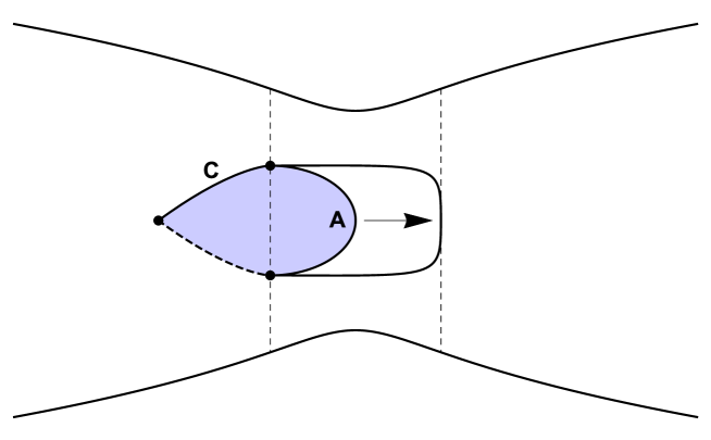
Figure 4: Well-posed characteristic problem for a mixed-type partial differential equation: The function is specified on one characteristic arc $C$ of the equation in the Lorentzian phase and on an arc $A$ in the Euclidean phase connecting the endpoints of $C$ and of a second characteristic arc starting at the same point as $C$ (dashed). The data on the second characteristic arc are determined for solutions of (1) and cannot be chosen freely.

In order to address differentiability, a Tricomi-style characteristic problem is more appropriate. In the Lorentzian phase, one specifies data not on initial-value surfaces but on characteristics of the differential equation as long as it is hyperbolic. Far away from the border with the Euclidean region, these characteristics are standard light rays, but they approach the border normal to constant-$t$ surfaces and end there. One example is shown as curve $C$ in Fig. 4. Considering just one spatial dimension, a second characteristic starting from the same point as $C$ completes the first one to a characteristic triangle with the two characteristics as well as the enclosed border with the Euclidean region as its sides.

The problem is well-posed [7, 32] if one specifies the field $\phi$ on one of the two characteristics and on an arc $A$ which starts and ends at the border-endpoints of the two characteristics but stays in the Euclidean region in between. If these data are smooth on the curve obtained as the union of $C$ and $A$ one obtains a unique, stable and smooth solution in the interior of the union of the characteristic triangle and the region enclosed by the curve $A$. Smoothness is guaranteed in this way, with data on the curve $A$ being completely free except that they must extend the data on $C$ smoothly. The indeterministic behavior (requiring future data) is therefore confirmed. If one lets $A$ approach the other border of the Euclidean region, one can proceed as in the intuitive description based on Fig. 3. An initial-value problem starting at the beginning of the expanding phase is then well-posed toward the future.

In four dimensions, the characteristic triangle is extended to the interior of the future light cone starting somewhere in the collapse phase, and the region enclosed by a curve $A$ is extended to a dome enclosed by a 3-dimensional hypersurface in the Euclidean region. Although we are not aware of a complete mathematical proof, one may expect the characteristic problem to be well-posed with data given by the mode on half the light cone and on the hypersurface in the Euclidean region.

The smoothness of solutions shows that there is still a well-defined manifold which combines the two Lorentzian phases and the Euclidean phase, but this manifold is no longer Riemannian. Standard obstacles to signature change in general relativity therefore do not apply. The use of a finite region in the characteristic formulation does not cause a problem in cosmology because we always have observational access to a finite part of our universe. The characteristic triangle can always be chosen large enough to include the whole observational range.

4.2.3 Boundary conditions at the hypersurface of signature change

Besides the boundary, initial-value and the characteristic problems discussed in the previous subsection we would like to present one more possibility of posing the initial-value problem for the evolution in the Lorentzian domain. Let us start by finding the solution in the Euclidean domain.

In this domain (which we call $\Omega_{E}$) the equations of motion are of the elliptic type. Therefore, for finding solutions in a subset $\Omega\subset\Omega_{E}$ the proper boundary conditions have to be imposed. Specifying $\phi|_{\partial\Omega}$ (where $\partial\Omega$ is the boundary of $\Omega$) is sufficient to determine a solution $\phi_{E}$ to the elliptic equation in the domain $\Omega$ uniquely. An interesting situation corresponds to the case when the boundary $\partial\Omega$ is expanded so that it encloses the whole Euclidean domain: $\partial\Omega\rightarrow\partial\Omega_{E}$. Such a boundary can be decomposed as follows $\partial\Omega_{E}=\partial\Omega_{+}+\partial\Omega_{-}+\partial\Omega_{\infty}$. The $\partial\Omega_{\pm}$ are boundaries between the Euclidean and Lorentzian domains at $\pm t_{\rm max}$, respectively, while $\partial\Omega_{\infty}$ encloses the Euclidean domain at spatial infinity (assuming that the space part is unbounded). The solution $\phi_{E}$ at $\Omega_{E}$ obtained by imposing boundary (Dirichlet or von Neumann) conditions at $\partial\Omega_{E}$ can now be used to determine initial (or final) conditions for the Lorentzian sectors $\Omega_{\pm}$, where $``+"$ corresponds to $t>+t_{\rm max}$ and $``-"$ to $t<-t_{\rm max}$. The $\pm t_{\rm max}$ (as previously) are the times at which signature change is taking place.

Let us decide to impose the Dirichlet boundary condition $\phi_{E}|_{\partial\Omega_{E}}$, leading to a solution $\phi_{E}$. Then, the Cauchy initial conditions at $\pm t_{\rm max}$ for the solutions $\phi_{L\pm}$ in the Lorentzian domains $\Omega_{L\pm}$ respectively are:

$$\lim_{t\rightarrow\pm{t_{\rm max}}^{\pm}}\phi_{L\pm} = \phi_{E}|_{\partial\Omega_{\pm}}\equiv\phi_{\pm},$$ (38)

$$\lim_{t\rightarrow\pm{t_{\rm max}}^{\pm}}\frac{\partial\phi_{L}}{\partial t} = \lim_{t\rightarrow\pm{t_{\rm max}}^{\mp}}\frac{\partial\phi_{E}}{\partial t}\,.$$ (39)

In this way by solving the equation of motion in the whole Euclidean domain, the initial (or final) data for evolution in the Lorentzian sector can be recovered. It is worth stressing that, as already discussed in the previous subsection, the continuity of solutions up to at least second time derivatives is required. (The equations are of second order.) The additional conditions

$$\lim_{t\rightarrow\pm{t_{\rm max}}^{\pm}}\frac{\partial^{2}\phi_{L}}{\partial t^{2}}=\lim_{t\rightarrow\pm{t_{\rm max}}^{\mp}}\frac{\partial^{2}\phi_{E}}{\partial t^{2}}$$ (40)

therefore have to be satisfied. In general, one can expect that only a subset of all possible boundary values $\phi_{E}|_{\partial\Omega_{E}}$ obey this condition. Such a possibility might be attractive because it may put restrictions on the form of the allowed boundary conditions, based on the requirement of mathematical consistency. For the typical equation of motion under consideration, Eq. (1), the requirement (40) leads to the following condition of continuity of the source term

$$\lim_{t\rightarrow\pm{t_{\rm max}}^{\pm}}S[\phi_{L\pm}]=\lim_{t\rightarrow\pm{t_{\rm max}}^{\mp}}S[\phi_{E}]\,.$$ (41)

In order to illustrate some features of the method discussed above, let us study the equation of motion

$$\frac{\partial^{2}\phi}{\partial t^{2}}-\beta(t)\frac{\partial^{2}\phi}{\partial x^{2}}=0\,,$$ (42)

with the step-like $\beta$-function

$$\beta(t)=\left\{\begin{array}[]{ccc}1&{\rm for}&t>t_{\rm max}\,,\\ -1&{\rm for}&t_{\rm max}\geq t\geq-t_{\rm max}\,,\\ 1&{\rm for}&t<-t_{\rm max}\,.\end{array}\right.$$ (43)

In this (1+1)-dimensional example the variation of $\beta$ is not continuous across the signature change, therefore condition (40) will have no chance of being fulfilled. Nevertheless, let us choose the following boundary conditions:

$$\phi_{\pm}=c_{\pm}\cos(x)\,,$$ (44)

where $c_{\pm}\in\mathbb{R}$ are constants. (The boundary condition at $\partial\Omega_{\infty}$ will not play any role.) With boundary values specified, a solution to Eq. (42) in the Euclidean domain $\Omega_{E}=\left\{(t,x)\in\mathbb{R}^{2},t_{\rm max}\geq t\geq-t_{\rm max}\right\}$ can be found:

$$\phi_{E}=\cos(x)\frac{c_{+}{\rm sh}(t+t_{\rm max})-c_{-}{\rm sh}(t-t_{\rm max})}{{\rm sh}(2t_{\rm max})}\,.$$ (45)

Using the solution we can find that

$$\lim_{t\rightarrow\pm{t_{\rm max}}^{\mp}}\frac{\partial\phi_{E}}{\partial t}=\cos(x)\frac{\mp c_{\mp}\pm c_{\pm}{\rm ch}(2t_{\rm max})}{\sinh(2t_{\rm max})}\,,$$ (46)

which will be used to impose Cauchy initial conditions in the Lorentzian domains. Taking this into account, solutions to Eq. (42) in the domains $\Omega_{\pm}=\left\{(t,x)\in\mathbb{R}^{2},\pm t>t_{\rm max}\right\}$ can be determined:

$$\phi_{L+} = \cos(x)\frac{c_{+}\left({\rm sh}(2t_{\rm max})\cos(t-t_{\rm max})+{\rm ch}(2t_{\rm max})\sin(t-t_{\rm max})\right)-c_{-}\sin(t-t_{\rm max})}{{\rm sh}(2t_{\rm max})}\,,$$

$$\phi_{L-} = \cos(x)\frac{c_{-}\left({\rm sh}(2t_{\rm max})\cos(t+t_{\rm max})-{\rm ch}(2t_{\rm max})\sin(t+t_{\rm max})\right)+c_{+}\sin(t+t_{\rm max})}{{\rm sh}(2t_{\rm max})}\,.$$

The solutions $\phi_{E}$ and $\phi_{L\pm}$ are presented in Fig. 5 in the form of the density plot for the sample values of $c_{\pm}$ and $t_{\rm max}$.

Figure 5: Density plot of the solutions $\phi_{E}$ and $\phi_{L\pm}$ to the equation (42). The observed asymmetry is due to the different boundary conditions at $t_{\rm max}$ and $-t_{\rm max}$: $\phi_{\pm}=c_{\pm}\cos(x)$. The values $c_{+}=1$, $c_{-}=2$ and $t_{\rm max}=4$ have beed used.

The solutions obtained in this way are regular in the whole domain $\Omega=\Omega_{E}\cup\Omega_{+}\cup\Omega_{-}$. However, in agreement with the earlier expectations, the second derivatives are discontinuous across the signature change:

$$\lim_{t\rightarrow\pm{t_{\rm max}}^{\mp}}\frac{\partial^{2}\phi_{E}}{\partial t^{2}}-\lim_{t\rightarrow\pm{t_{\rm max}}^{\pm}}\frac{\partial^{2}\phi_{L\pm}}{\partial t^{2}}=2c_{\pm}\cos(x)\,.$$ (49)

4.2.4 Wave functions

Mixed-type differential equations for modes are a consequence of properties of effective equations in cosmological models of loop quantum gravity. These properties follow from a general analysis of consistent and anomaly-free realizations of field equations, so that physical predictions made in these models are independent of coordinate or gauge choices. The same modifications to space-time structure can be seen from commutator algebras at the quantum level, but it is then more difficult to derive dynamical effects. It is nevertheless interesting to discuss how signature change or its accompanying instabilities could be seen in the evolution of wave functions.

As long as one has unitary evolution, as can easily be guaranteed in deparameterized models which provide the majority of explicit wave-function evolutions in quantum cosmology, the wave function cannot be subject to instabilities. (However, we note that at a fundamental level it may be difficult to have unitary evolution under all circumstances, owing to the problem of time.) Its norm is preserved even throughout high density. Accordingly, the Schrödinger or Klein–Gordon type equation which the wave function is subject to does not change its form to become elliptic; the relevant coefficients in the wave equation do not change sign. After all, what changes is the signature of space(-time), not the signature of (mini)superspace on which the wave function is defined. (See also [40]. In fact, depending on which representation one chooses for the wave function, the equation it is subject to may be elliptic or hyperbolic even for standard space-time.)

Signature change implies instabilities in an initial-value problem for the modes, solving effective equations. The fields in effective equations are expectation values of mode operators in a state obeying the equation for the wave function. At the level of wave-function evolution, signature change would therefore be recognized in an exponential change of expectation values of mode operators. (If wave packets are used, their peak position would change exponentially.) For these expectation values (or peak positions), the same sensitivity to initial values as observed in solutions of effective equations would occur, even if they are computed from an evolved wave function. These observable quantities therefore evolve in an unstable way, causing the same problem as seen in an initial-value formulation for effective equations. Instability problems are just more hidden in schemes that first evolve wave functions and then compute expectation values, but they are just as pressing as in effective equations.

In this respect, the situation is reminiscent of quantum chaos, which, compared with the classical phenomenon, is more difficult to define and discuss, but not absent, for wave functions subject to linear differential equations. In both cases, the sensitivity of evolved expectation values to initial choices is relevant. It has been discussed in detail in the context of quantum chaos. Following [41, 42], we can use the same arguments for states in the presence of signature change: Unitary quantum evolution ensures that the overlap $|\langle\psi_{1}(t),\psi_{2}(t)\rangle|^{2}$ of two different initial states $\psi_{1}(t_{0})$ and $\psi_{2}(t_{0})$ is conserved in time, and therefore does not indicate any sensitivity to choices of initial values. However, quantum evolution of classically chaotic systems is very sensitive to perturbations of the Hamiltonian operator, in the sense that the overlap $|\langle\psi_{1}(t),\psi_{2}(t)\rangle|^{2}$ changes rapidly if $\psi_{1}(t)$ and $\psi_{2}(t)$ are now defined as states evolved from the same initial wave function $\psi_{1}(t_{0})=\psi_{2}(t_{0})$ but with different Hamiltonians $\hat{H}_{1}=\hat{H}$ and $\hat{H}_{2}=\hat{H}+\epsilon\hat{V}$ with some small $\epsilon$ and a perturbation potential $\hat{V}$. Similarly, the same definition of the overlap in Euclidean signature leads to rapid (exponential) change because the perturbed evolution by $\hat{H}_{2}$ contains a factor of $\exp(\epsilon\hbar^{-1}\hat{V}t)$. In discussions of quantum chaos, $\epsilon\hat{V}$ is usually thought of as coming from unknown interactions with an environment hard to control. The same source of $\epsilon\hat{V}$ exists in quantum cosmology because the precise degrees of freedom and interactions at high density are not well known. In addition to this, loop quantum gravity is subject to a large set of quantization ambiguities, so that the dynamics is not precisely determined and a second source of $\epsilon\hat{V}$ results.

Signature change in effective equations, in all existing models, is implied by the requirement of anomaly freedom, so that predictions are guaranteed to be independent of gauge choices. Most models in which one evolves wave functions are based on deparameterization, in which one formulates “evolution” of a wave packet in terms of a so-called internal time, which is not a coordinate but one of the dynamical fields. The conditions on well-defined evolution after deparameterization are less severe than the general covariance conditions when one does not select a specific time, be it a coordinate or internal. If one were to fix the gauge and work in one specific set of coordinates, one could avoid having to use effective equations subject to signature change. Similarly, the possibility of formulating stable wave-function dynamics in one chosen internal time does not mean that wave functions in general evolve in a stable manner. One would have to show, first, that predictions of one’s model do not depend on which field is chosen as internal time (a task which has not been performed in deparameterized models of quantum cosmology; see [43, 44]). After this, one could reliably analyze evolution and test whether it is always meaningful or has to be stopped when a Euclidean regime is reached. Performing this task turns out to be much more complicated than analyzing anomaly freedom of effective equations. But interestingly, even in the absence of such an analysis there are hints that wave-function evolution becomes unstable at high density, in the sense that expectation values of modes change exponentially [45].

4.2.5 Cosmological implications

A well-posed treatment of initial and boundary values in loop quantum cosmology implies significant departures from the scenarios commonly made in this setting. For instance, there has been some interest in a “super-inflationary” phase at high density, around a bounce, during which the Hubble parameter grows quickly [46]. Although the rapid change happens for background variables and is therefore not the same as the instabilities of mode equations such as (1), one can easily check in explicit models that the super-inflationary phase falls within the elliptic range of the partial differential equations for inhomogeneity [5]. The rapid growth of background variables cannot be used for cosmological effects because their values at the border of the Euclidean phase must be prescribed as part of the boundary-value problem. Obtaining a large parameter with an ill-posed initial-value problem does not have physical significance.

A related effect has been seen in a combination of loop-modified background equations with inflationary models: At high density, the modified equation for the inflaton has an anti-friction term which can easily push the inflaton up to a high value in its potential [47, 48]. Given the right potential for suitable inflation, the correct initial conditions can therefore be provided. Also this effect is subject to the verdict of being based on ill-posed data. An alteration may, however, still be realized if one can show that for a given background value $\bar{\phi}$ at the beginning of the expansion phase there must generically be a large $\bar{\phi}^{\prime}$ according to the well-posed characteristic formulation. Values of $\bar{\phi}$ far from the minimum of a potential could then be achieved afterwards, using well-posed evolution with the predicted initial values in the expansion phase.

With the discussion of initial and boundary values in Sec. 4.2.2, we can make our expectations for cosmological scenarios more precise. Some data must be chosen at the beginning of the expansion phase, even if the energy density or other coefficients of the differential equation never become infinite. This feature is shared with the singular big-bang model, in which the main conceptual problem is caused not so much by divergences but rather by the presence of unrestricted initial data. (In general relativity, it is possible to extend solutions across singularities in a distributional sense, but the extension is not unique [49].) If there would be a unique way of deriving initial values at the beginning of the expansion phase, the singularity of the traditional big-bang model would not be so much of a problem. One could make clear predictions about the initial state and further evolution of the universe, as attempted in inflationary scenarios with their (somewhat controversial) initial conditions for the inflaton. In practical terms, the singularity problem is therefore one of indeterminedness, which is implied but not necessarily equivalent to the occurrence of divergences.

An example for the latter part of the preceding statement is given by signature-change cosmology. There are no divergences in these models, and yet an important part of initial values for the expansion phase remains free. The resulting scenario, which we call a finite beginning to emphasize the absence of divergences together with the requirement of choosing new initial values, is rather close to the standard big-bang model. In particular, for practical purposes the need for new initial values once the density is sufficiently low to trigger signature change back to a Lorentzian structure makes the Euclidean region appear as a singularity. We therefore speak of a finite beginning instead of a non-singular one, keeping in mind that the main problem of a singularity is the indeterminedness of initial data.

There may yet be a crucial difference with the standard big-bang model: What we need to prescribe at the finite beginning, according to Fig. 3, is only the field $\phi$, not its normal derivative $\phi^{\prime}$ if we start evolution in the collapse phase. If one has some means to know $\phi$ in a neighborhood of the border between the Euclidean region and the expansion phase, for instance from some hypothetical observations, one can derive $\phi^{\prime}$ and draw conclusions about the field in the collapse phase. There is therefore some connection between collapse and expansion, although it is not causal and not fully deterministic. A thorough cosmological analysis of scalar and tensor power spectra in signature-change models is required before one can tell how much about the collapse phase could be deciphered in this indirect way.

4.2.6 Global issues

While effective methods for constrained systems provide reliable local equations, as confirmed by the results of this paper, there may seem to be several global problems related to the new type of partial differential equations which imply the disappearance of time or causality at high density. One example has been discussed in [51] in the context of black holes, where the non-singular beginning in cosmology as detailed here is replaced by a naked singularity (again in the sense of indeterminism) with a Cauchy horizon. Even if local field equations are regular, the lack of a causal structure in some regions may lead to unacceptable indeterministic behavior at a global level.

A different kind of global problem is indicated by one feature of solutions to Tricomi’s problem which we have not mentioned so far. Again, locally the equation and its solutions are well-defined. But generic solutions turn out to have a pole at one point $A\cap B$ in Fig. 4, where the Euclidean arc ends [7]: Although solutions are smooth in the interior of the characteristic region (for smooth boundary data) most of them have a pole at one endpoint of the boundary. (This result explains the ubiquity of sonic booms in analogous acoustic models.) The solution may remain finite, but not all of its derivatives do. Derived quantities such as the energy density in a matter field could therefore diverge. If this happens, it is not likely that cosmological perturbation theory gives reliable results, even though the local perturbative equations are regular.

The acoustic analog illustrates a further point: One could think that signature change in cosmology (or black-hole physics) is harmless because analogous effects can appear in well-known systems such as transonic motion (or the model discussed in Sec. 3.2). The difference is that transonic motion leads to signature change only for excitations in the fluid, while all other propagating degrees of freedom including the bulk fluid motion and space-time are still governed by deterministic equations. (The speed of light is an absolute limit for any causal motion, very much unlike the speed of sound in a fluid. If $\beta<0$ in (1), all motion is eliminated.) If the bulk of the fluid is forced to move faster than its own speed of sound, it overtakes any sound wave generated in it, so that its density profile provides future conditions for the wave. Mathematically, this is represented by Tricomi’s future data. However, the bulk fluid itself moves in a deterministic (but not wave-like) way even if it is faster than its own speed of sound, and no causality issues appear. The situation is very different when signature change happens for space-time physics, in which case no reference time remains to define a causal structure and no mode can evolve deterministically. For this reason, signature change in effective space-time models of loop quantum gravity has much more radical consequences than analogous effects in matter systems, as discussed in the present paper as well as [51].

5 Conclusions

We have described several fundamental properties of a new scenario, based on signature change, that has emerged from spherically symmetric and cosmological models of loop quantum gravity in recent years. We emphasize that this scenario cannot be seen in the minisuperspace models traditionally studied in loop quantum cosmology [52]. In fact, the possibility of signature change casts significant doubt on the viability of minisuperspace models of loop quantum cosmlogy because in such models one would not see any sign of a disappearing causal structure at high density. Minisuperspace models of loop quantum cosmology may be used for some estimates of background properties, but they can no longer be considered as reliable sources of stand-alone cosmological scenarios. One always has to go beyond homogeneity to make sure that there is a well-defined space-time structure and to check whether mode equations remain hyperbolic, or to exclude other exotic effects.

Signature-change cosmology is therefore a new scenario which crucially relies on inhomogeneous features of loop quantum gravity (even though, needless to say, it has not yet been derived from a full quantization of gravity). Its details, regarding for instance power spectra, still have to be worked out, but we believe that the more mathematical and conceptual properties discussed in this article already show a large number of interesting features. The main consequence in practical terms is the occurrence of instabilities, related to the sensitive dependence of solutions on initial data. In some examples, instabilities may be physical effects which imply rapid change but no inconsistencies. In quantum gravity, however, instabilities of the kind encountered in the presence of signature change are fatal: The theory remains subject to a large number of quantization ambiguities in its equations, and not much is known about suitable initial states for quantum space (and not just quantum matter). With this inherent vagueness, one cannot afford any instabilities that would magnify theoretical uncertainties in a short amount of time, even if this time may be as small as the Planck time. No predictions would be possible. We are therefore sympathetic with the verdict “In light of the fact that even this ’well-behaved’ signature change system predicts its own downfall, it may be prudent to reassess the inclusion of signature changing metrics in quantum gravity theories.” [53] obtained after a detailed analysis of initial-value problems in a model of classical signature change. Our model is provided by effective equations of loop quantum gravity in which signature change appears to be generic (and is not included by choice). The verdict of [53] can therefore be applied to loop quantum gravity at least to the extent that extreme caution is called for when one considers evolution through high density.

In the presence of signature change, instabilities can be avoided only if one switches to a 4-dimensional boundary-value problem at high density, giving up causality. Although ambiguities remain in the theory, there are several qualitative effects with interesting implications. As one of the main observations in this article, the mixed-type partial differential equations for modes in this context strike a nice balance between deterministic cyclic models and singular big-bang models. There are no divergences, and yet initial data in the infinite past do not uniquely determine all of space(-time). For every mode, one must specify one function at the beginning of the expansion phase even if one has already chosen initial values for the contraction phase. Still, the normal derivative of the field is not free and may carry subtle but interesting information about the pre-big bang.

Appendix A Space-time

We present here a somewhat technical discussion of fundamental properties of space-times underlying (1). Symmetries and gauge transformations are especially important in this context, as well as properties of the canonical formulation of gravity. In our following exposition, we also provide more details on the derivation and reliability of equations such as (1) in effective models of loop quantum gravity.

A.1 Gauge transformations

In spite of its appearance, equation (1) is covariant in a generalized sense, according to an effective (and canonically defined) non-Riemannian structure of quantum space-time. The usual Lorentz and Poincaré symmetries, under which the classical version of (1) with $\beta=1$ (and constant $a$) would be invariant, are realized in canonical gravity as a subalgebra of the infinite-dimensional algebra (or rather, algebroid [54]) of deformations of 3-dimensional spacelike hypersurfaces in space-time. (See for instance [55, 56].) These hypersurface deformations are gauge transformations of any generally covariant theory, including gravity.

Hypersurface deformations [8] are more suitable than Poincaré transformations in situations in which no background space-time metric is assumed. They provide the proper framework for a discussion of generalized space-time structures as the may be implied by canonical quantum gravity. Hypersurface deformations have an infinite set of generators, spatial ones given by $D[N^{a}]$ with spatial vector fields $N^{a}$ tangential to the hypersurface, and normal ones $H[N]$ with functions $N$ on the hypersurface so that the deformation is by an amount $Nn^{a}$ along the unit normal $n^{a}$. The classical space-time geometry [8] (as well as the canonical form of general relativity [57]) imply that these generators have commutators (or classical Poisson brackets)

$$\{D[N_{1}^{a}],D[N_{2}^{b}]\} = D[N_{1}^{a}{\rm D}_{b}N_{2}^{b}-N_{2}^{a}{\rm D}_{a}N_{1}^{b}]$$ (50)

$$\{H[N],D[N^{a}]\} = H[N^{a}{\rm D}_{a}N]$$ (51)

$$\{H[N_{1}],H[N_{2}]\} = -D[h^{ab}(N_{1}{\rm D}_{b}N_{2}-N_{2}{\rm D}_{b}N_{1})]$$ (52)

with the induced metric $h_{ab}$ and covariant derivative ${\rm D}_{a}$ on a hypersurface.

When one tries to quantize the theory canonically, one should turn the gauge generators into operators, so that they still have closed brackets given by commutators. Otherwise, the classical gauge transformations would be broken and the quantum theory would not be consistent; it would have gauge anomalies. The anomaly problem of canonical quantum gravity is important, but also very difficult and unresolved so far. (One reason is the presence of the metric in (52), which at the quantum level would be an operator and give rise to complicated ordering questions with a quantized $D[N^{a}]$.) Nevertheless, there have been several independent indications in recent years which give some hope that the problem can be solved. At the operator level, especially $2+1$-dimensional models have been analyzed in quite some detail, paying attention to the full algebra of gauge generators. Consistent versions have been found in different ways [58, 59, 60, 61], including also spherically symmetric models [62].

Independently, effective calculations start from the observation that the quantum operation of commutators together with a closed algebra of operators $\hat{C}_{I}$, $[\hat{C}_{I},\hat{C}_{J}]=\hat{f}^{K}_{IJ}\hat{C}_{K}$ with structure constants (or functions/operators) $\hat{f}^{K}_{IJ}$, implies a closed algebra under Poisson brackets of effective constraints $\langle\hat{C}_{I}\rangle$. These effective constraints are defined as expectation values $\langle\hat{C}_{I}\rangle$ of the constraint operators in an arbitrary state [63, 64]. Effective constraints are therefore functions on the quantum state space, which can conveniently be parameterized by expectation values and moments with respect to a set of basic operators. In addition to these effective constraints, obtained as direct expectation values of constraint operators, there is an infinite set of independent ones, derived from the same constraint operators as $\langle\widehat{\rm pol}\hat{C}_{I}\rangle$ for all polynomials in basic operators. All these functions on the space of states would be zero on the subspace annihilated by the constraints $\hat{C}_{I}$, imposed following Dirac’s prescription. The need for an infinite set of effective constraints for every single constraint operator follows from the requirement that a whole tower of infinitely many moments must be constrained together with every constrained expectation value.

A Poisson bracket on the quantum state space of expectation values and moments can be defined by $\{\langle\hat{A}\rangle,\langle\hat{B}\rangle\}=\langle[\hat{A},\hat{B}]\rangle/i\hbar$, extended by the Leibniz rule to products of expectation values (as they appear in quantum fluctuations and higher moments). With these definitions, it follows that effective constraints form a closed algebra under Poisson brackets if the constraint operators form a closed algebra under commutators. Practically, it is easier to evaluate Poisson brackets than commutators, an observation on which the idea of canonical effective equations [65, 66] and constraints [63, 64] is based. Also, there are useful approximation schemes, such as a semiclassical one in which one would do calculations order by order in the moments, which are easier to implement for effective constraints than for constraint operators and allow one to handle the unwieldy space of all states more efficiently. For finite orders in the moments, there is a finite number of independent effective constraints, and the task of computing their algebra becomes feasible.

If we have a closed algebra $[\hat{C}_{I},\hat{C}_{J}]$ of operators, the corresponding effective constraints truncated at some moment order form a closed Poisson-bracket algebra up to this order, irrespective of the states used. This formulation of effective theories is therefore much more general than the usual idea of effective actions [67]. (The latter are often combined with further approximations such as derivative expansions, or with restrictions of states such as near-vacuum states for the low-energy effective action.) In our case, we need not make any assumption on the class of states in order to obtain a closed algebra of effective constraints. One may just have to include higher orders in the moments for a better approximation to solutions corresponding to strong quantum states; but even at lower orders, the algebra must be closed (to within the same order). Effective constraints therefore provide a good test of possible anomaly-free quantum constraint algebras. In particular, if one can show that no closed effective constraint algebra exists to within some order in moments, using a large-enough parameterization of quantum corrections, there cannot be a closed algebra of constraint operators. And if closure of effective constraints can be achieved only if the classical constraint algebra is modified, the full quantum constraint algebra must be subject to quantum corrections which change the form of gauge transformations. Signature change is just one of the consequences found in this way: Instead of (52), we then have

$$\{H[N_{1}],H[N_{2}]\}=-D[\beta h^{ab}(N_{1}{\rm D}_{b}N_{2}-N_{2}{\rm D}_{b}N_{1})]$$ (53)

with a phase-space function $\beta$ which may turn negative (while the other brackets involving $D[N^{a}]$ remain unchanged). Canonical field equations consistent with this modified bracket are of the form (1), as shown by [5] using the methods of [8, 68]. (The same modification of derivative terms is realized to higher orders in derivatives [69].)

So far, calculations in models of loop quantum gravity have been performed only to zeroth order in the moments. But they still show interesting effects because, in addition to moment terms, the theory implies further quantum corrections. At high density, holonomy modifications are relevant, which are implied by the basic assumption of loop quantum gravity [70, 71, 72] that the gravitational connection can be represented as an operator only when it is integrated and exponentiated to a holonomy. A second effect, inverse-triad corrections [73, 74, 9], is more indirect but also related to the basic assumption. It implies corrections relevant at lower curvature [9, 75, 76]. Effective constraint algebras have been computed in both cases and found to allow for consistent versions: [77, 78, 79] as examples for inverse-triad corrections, [3] for holonomy corrections, and [1, 4, 2] for combinations of both. Whenever holonomy modifications are present, all generic consistent effective constraints found so far imply mode equations of the form (1).

The derivation shows that covariance is not broken because all classical gauge generators have a valid analog as a constraint operator $\hat{C}_{I}$ or as an effective constraint. For every classical gauge transformation, there is a corresponding quantum or effective gauge transformation. No transformations are violated, including the Lorentz and Poincaré ones that one obtains as a special case of hypersurface deformations [55]. Nevertheless, it is possible for (1) to differ from standard covariant wave equations because quantum gauge generators, while they must not be broken for an anomaly-free theory, may be subject to quantum corrections. These corrections can be seen in the structure operators or functions $\hat{f}^{K}_{IJ}$ of the quantum or effective constraint algebras. For holonomy and inverse-triad corrections, the classical structure functions are, as in (53), multiplied with a phase-space function $\beta$, which determines a new consistent form of quantum space-time covariance. The same function appears in mode equations (1) derived from the effective constraints.

A.2 Slicing independence

Even though the speed in (1) provided by quantum geometry depends on the spatial metric and extrinsic curvature — quantities that are not covariant in classical space-time — the effect is frame independent in a subtle way. The models in which such modified speeds have been derived are anomaly free, so that the classical set of gauge transformations (given by coordinate changes) is not violated. However, not just the dynamics but also the structure of space-time receives quantum corrections. There is a new set of gauge transformations under which the quantum-corrected field equations are invariant, and which has the full set of standard coordinate changes as its classical limit. The effective theories, including modified speeds they predict, are covariant under these deformed gauge transformations. Accordingly, the space-time structure is no longer classical or Riemannian, but it remains well-defined in canonical terms.

Put differently, one could worry that models in which waves propagate with speeds depending on the spatial metric and extrinsic curvature of constant-time hypersurfaces violate the slicing independence of the classical theory. Classically, for any given space-time, one can, depending on one’s set of coordinates, choose equal-time slices with large or small extrinsic curvature, even if the covariant curvature of space-time vanishes. A speed depending on extrinsic curvature would then suggest that predictions depend on the slicing or the choice of an initial-value surface, which would be unacceptable. This worry is unjustified because the two initial-value surfaces, one with small and one with large extrinsic curvature, would give rise to different physical solutions of the effective theory even though they would present the same classical solution. Predictions, for instance of the speed, then differ simply because one would consider physically different solutions. Transformations between different slicings are, just like coordinate changes, gauge transformations which are modified in the effective theory. Slicings of one and the same classical space-time, which are related by classical gauge transformations, are not gauge related in the quantum-corrected setting.

References

- [1] J. D. Reyes, Spherically Symmetric Loop Quantum Gravity: Connections to 2-Dimensional Models and Applications to Gravitational Collapse, PhD thesis, The Pennsylvania State University, 2009
- [2] M. Bojowald, G. M. Paily, and J. D. Reyes, Discreteness corrections and higher spatial derivatives in effective canonical quantum gravity, Phys. Rev. D 90 (2014) 025025, [arXiv:1402.5130]
- [3] T. Cailleteau, J. Mielczarek, A. Barrau, and J. Grain, Anomaly-free scalar perturbations with holonomy corrections in loop quantum cosmology, Class. Quant. Grav. 29 (2012) 095010, [arXiv:1111.3535]
- [4] T. Cailleteau, L. Linsefors, and A. Barrau, Anomaly-free perturbations with inverse-volume and holonomy corrections in Loop Quantum Cosmology, Class. Quantum Grav. 31 (2014) 125011, [arXiv:1307.5238]
- [5] M. Bojowald and G. M. Paily, Deformed General Relativity and Effective Actions from Loop Quantum Gravity, Phys. Rev. D 86 (2012) 104018, [arXiv:1112.1899]
- [6] J. B. Hartle and S. W. Hawking, Wave function of the Universe, Phys. Rev. D 28 (1983) 2960–2975
- [7] F. G. Tricomi, Repertorium der Theorie der Differentialgleichungen, Springer Verlag, 1968
- [8] S. A. Hojman, K. Kuchař, and C. Teitelboim, Geometrodynamics Regained, Ann. Phys. (New York) 96 (1976) 88–135
- [9] M. Bojowald and G. Calcagni, Inflationary observables in loop quantum cosmology, JCAP 1103 (2011) 032, [arXiv:1011.2779]
- [10] G. F. R. Ellis, A. Sumeruk, D. Coule, and C. Hellaby, Change of signature in classical relativity, Class. Quantum Grav. 9 (1992) 1535–1554
- [11] L. C. Gomar and G. A. Mena Marugán, Uniqueness of the Fock quantization of scalar fields and processes with signature change in cosmology, [arXiv:1403.6984]
- [12] G. F. R. Ellis, A. Sumeruk, D. Coule, and C. Hellaby, Change of signature in classical relativity, Class. Quantum Grav. 9 (1992) 1535–1554
- [13] T. Dray, G. F. R. Ellis, C. Hellaby, and C. A. Manogue, Gravity and signature change, Gen. Rel. Grav. 29 (1997) 591–597, [gr-qc/9610063]
- [14] M. Kossowski and M. Kriele, Signature type change and absolute time in general relativity, Class. Quantum Grav. 10 (1993) 1157–1164
- [15] M. Kossowski and M. Kriele, Smooth and discontinuous signature type change in general relativity, Class. Quantum Grav. 10 (1993) 2363–2371
- [16] S. A. Hayward, Junction Conditions for Signature Change, [gr-qc/9303034]
- [17] T. Dray, C. A. Manogue, and R. W. Tucker, Boundary conditions for the scalar field in the presence of signature change, Class. Quantum Grav. 12 (1995) 2767–2777
- [18] M. Carfora and G. Ellis, The Geometry of classical change of signature, Int. J. Mod. Phys. D 4 (1995) 175–188, [gr-qc/9406043]
- [19] J. F. Barbero G., From Euclidean to Lorentzian General Relativity: The Real Way, Phys. Rev. D 54 (1996) 1492–1499, [gr-qc/9605066]
- [20] A. Barrau, M. Bojowald, G. Calcagni, J. Grain, and M. Kagan, Anomaly-free cosmological perturbations in effective canonical quantum gravity, [arXiv:1404.1018]
- [21] S. Yoshida, B. C. Bromley, J. S. Read, K. Uryu, and J. L. Friedman, Models of helically symmetric binary systems, Class. Quantum Grav. 23 (2006) S599–S614, [gr-qc/0605035]
- [22] S. Carlip, Real tunneling solutions and the Hartle–Hawking wavefunction, Class. Quantum Grav. 10 (1993) 1057–1064
- [23] M. Bojowald, Loop Quantum Cosmology IV: Discrete Time Evolution, Class. Quantum Grav. 18 (2001) 1071–1088, [gr-qc/0008053]
- [24] M. Bojowald, Isotropic Loop Quantum Cosmology, Class. Quantum Grav. 19 (2002) 2717–2741, [gr-qc/0202077]
- [25] A. Vilenkin, Quantum creation of universes, Phys. Rev. D 30 (1984) 509–511
- [26] A. Poddubny, I. Iorsh, P. Belov, and Y. Kivshar, Hyperbolic metamaterials, Nature Photonics 7 (2013) 948Ð957
- [27] I. Smolyaninov and E. Narimanov, Metric Signature Transitions in Optical Metamaterials, Phys. Rev. Lett. 105 (2010) 067402
- [28] J. Pendry, Negative Refraction Makes a Perfect Lens, Phys. Rev. Lett. 85 (2000) 3966–3969
- [29] J. Mielczarek, Signature change in loop quantum cosmology, Springer Proc. Phys. 157 (2014) 555, [arXiv:1207.4657]
- [30] J. Mielczarek, Asymptotic silence in loop quantum cosmology, AIP Conf. Proc. 1514 (2012) 81, [arXiv:1212.3527]
- [31] J. Mielczarek, Big Bang as a critical point, [arxiv:1404.0228]
- [32] A. Weinstein, The singular solutions and the Cauchy problem for generalized Tricomi equations, Comm. Pure Appl. Math. 7 (1954) 105–116
- [33] G. Calcagni, B. de Carlos, and A. de Felice, Ghost conditions for Gauss–Bonnet cosmologies, Nucl. Phys. B 752 (2006) 404, [hep-th/0604201]
- [34] A. Ashtekar, T. Pawlowski, and P. Singh, Quantum Nature of the Big Bang, Phys. Rev. Lett. 96 (2006) 141301, [gr-qc/0602086]
- [35] M. Bojowald, Large scale effective theory for cosmological bounces, Phys. Rev. D 75 (2007) 081301(R), [gr-qc/0608100]
- [36] J. Mielczarek, T. Stachowiak, and M. Szydłowski, Exact solutions for big bounce in loop quantum cosmology, Phys. Rev. D 77 (2008) 123506, [arXiv:0801.0502]
- [37] M. Bojowald, How quantum is the big bang?, Phys. Rev. Lett. 100 (2008) 221301, [arXiv:0805.1192]
- [38] M. Bojowald, Fluctuation energies in quantum cosmology, Phys. Rev. D 89 (2014) 124031, [arXiv:1404.5284]
- [39] T. Cailleteau, A. Barrau, J. Grain, and F. Vidotto, Consistency of holonomy-corrected scalar, vector and tensor perturbations in Loop Quantum Cosmology, Phys. Rev. D 86 (2012) 087301, [arXiv:1206.6736]
- [40] J. Martin, Hamiltonian quantization of general relativity with the change of signature, Phys. Rev. D 49 (1994) 5086–5095
- [41] A. Peres, Stability of quantum motion in chaotic and regular systems, Phys. Rev. A 30 (1984) 1610–1615
- [42] R. A. Jalabert and H. M. Pastawski, Environment-independent decoherence rate in classically chaotic systems, Phys. Rev. Lett. 86 (2001) 2490–2493
- [43] P. Malkiewicz, Reduced phase space approach to Kasner universe and the problem of time in quantum theory, Class. Quantum Grav. 29 (2012) 075008, [arXiv:1105.6030]
- [44] P. Malkiewicz, Multiple choices of time in quantum cosmology, [arXiv:1407.3457]
- [45] D. Brizuela, G. A. Mena Marugán, and T. Pawlowski, Big Bounce and inhomogeneities, Class. Quantum Grav. 27 (2010) 052001, [arXiv:0902.0697]
- [46] E. J. Copeland, D. J. Mulryne, N. J. Nunes, and M. Shaeri, Super-inflation in Loop Quantum Cosmology, Phys. Rev. D 77 (2008) 023510, [arXiv:0708.1261]
- [47] M. Bojowald, Inflation from quantum geometry, Phys. Rev. Lett. 89 (2002) 261301, [gr-qc/0206054]
- [48] J. Mielczarek, The Observational Implications of Loop Quantum Cosmology, Phys. Rev. D 81 (2010) 063503, [arXiv:0908.4329]
- [49] S. W. Hawking and G. F. R. Ellis, The Large Scale Structure of Space-Time, Cambridge University Press, 1973
- [50] M. de Cervantes, Don Quixote, Putnam translation
- [51] M. Bojowald, Information loss, made worse by quantum gravity, [arXiv:1409.3157]
- [52] M. Bojowald, Loop Quantum Cosmology, Living Rev. Relativity 11 (2008) 4, [gr-qc/0601085], http://www.livingreviews.org/lrr-2008-4
- [53] L. J. Alty and C. J. Fewster, Initial Value Problems and Signature Change, Class. Quant. Grav. 13 (1996) 1129–1148, [gr-qc/9501026]
- [54] C. Blohmann, M. C. Barbosa Fernandes, and A. Weinstein, Groupoid symmetry and constraints in general relativity. 1: kinematics, Commun. Contemp. Math. 15 (2013) 1250061, [arXiv:1003.2857]
- [55] M. Bojowald and G. M. Paily, Deformed General Relativity, Phys. Rev. D 87 (2013) 044044, [arXiv:1212.4773]
- [56] M. Bojowald, Canonical Gravity and Applications: Cosmology, Black Holes, and Quantum Gravity, Cambridge University Press, Cambridge, 2010
- [57] P. A. M. Dirac, The theory of gravitation in Hamiltonian form, Proc. Roy. Soc. A 246 (1958) 333–343
- [58] A. Perez and D. Pranzetti, On the regularization of the constraints algebra of Quantum Gravity in dimensions with non-vanishing cosmological constant, Class. Quantum Grav. 27 (2010) 145009, [arXiv:1001.3292]
- [59] A. Henderson, A. Laddha, and C. Tomlin, Constraint algebra in LQG reloaded : Toy model of a Gauge Theory I, Phys. Rev. D 88 (2013) 044028, [arXiv:1204.0211]
- [60] A. Henderson, A. Laddha, and C. Tomlin, Constraint algebra in LQG reloaded : Toy model of an Abelian gauge theory - II Spatial Diffeomorphisms, Phys. Rev. D 88 (2013) 044029, [arXiv:1210.3960]
- [61] C. Tomlin and M. Varadarajan, Towards an Anomaly-Free Quantum Dynamics for a Weak Coupling Limit of Euclidean Gravity, Phys. Rev. D 87 (2013) 044039, [arXiv:1210.6869]
- [62] S. Brahma, Spherically symmetric canonical quantum gravity, [arXiv:1411.3661]
- [63] M. Bojowald, B. Sandhöfer, A. Skirzewski, and A. Tsobanjan, Effective constraints for quantum systems, Rev. Math. Phys. 21 (2009) 111–154, [arXiv:0804.3365]
- [64] M. Bojowald and A. Tsobanjan, Effective constraints for relativistic quantum systems, Phys. Rev. D 80 (2009) 125008, [arXiv:0906.1772]
- [65] M. Bojowald and A. Skirzewski, Effective Equations of Motion for Quantum Systems, Rev. Math. Phys. 18 (2006) 713–745, [math-ph/0511043]
- [66] M. Bojowald and A. Skirzewski, Quantum Gravity and Higher Curvature Actions, Int. J. Geom. Meth. Mod. Phys. 4 (2007) 25–52, [hep-th/0606232], Proceedings of “Current Mathematical Topics in Gravitation and Cosmology” (42nd Karpacz Winter School of Theoretical Physics), Ed. Borowiec, A. and Francaviglia, M.
- [67] M. Bojowald and S. Brahma, Effective constraint algebras with structure functions, [arXiv:1407.4444]
- [68] K. V. Kuchař, Geometrodynamics regained: A Lagrangian approach, J. Math. Phys. 15 (1974) 708–715
- [69] P. D. Cuttell and M. Sakellariadou, Fourth order deformed general relativity, Phys. Rev. D 90 (2014) 104026, [arXiv:1409.1902]
- [70] T. Thiemann, Introduction to Modern Canonical Quantum General Relativity, Cambridge University Press, Cambridge, UK, 2007, [gr-qc/0110034]
- [71] C. Rovelli, Quantum Gravity, Cambridge University Press, Cambridge, UK, 2004
- [72] A. Ashtekar and J. Lewandowski, Background independent quantum gravity: A status report, Class. Quantum Grav. 21 (2004) R53–R152, [gr-qc/0404018]
- [73] M. Bojowald, Inverse Scale Factor in Isotropic Quantum Geometry, Phys. Rev. D 64 (2001) 084018, [gr-qc/0105067]
- [74] M. Bojowald, H. Hernández, M. Kagan, and A. Skirzewski, Effective constraints of loop quantum gravity, Phys. Rev. D 75 (2007) 064022, [gr-qc/0611112]
- [75] M. Bojowald, G. Calcagni, and S. Tsujikawa, Observational test of inflation in loop quantum cosmology, JCAP 11 (2011) 046, [arXiv:1107.1540]
- [76] M. Bojowald, G. Calcagni, and S. Tsujikawa, Observational constraints on loop quantum cosmology, Phys. Rev. Lett. 107 (2011) 211302, [arXiv:1101.5391]
- [77] M. Bojowald, G. Hossain, M. Kagan, and S. Shankaranarayanan, Anomaly freedom in perturbative loop quantum gravity, Phys. Rev. D 78 (2008) 063547, [arXiv:0806.3929]
- [78] M. Bojowald, J. D. Reyes, and R. Tibrewala, Non-marginal LTB-like models with inverse triad corrections from loop quantum gravity, Phys. Rev. D 80 (2009) 084002, [arXiv:0906.4767]
- [79] A. Kreienbuehl, V. Husain, and S. S. Seahra, Modified general relativity as a model for quantum gravitational collapse, Class. Quantum Grav. 29 (2012) 095008, [arXiv:1011.2381]