Microscopic theory for electrocaloric effects in planar double layer systems

Abstract

We present a field theory approach to study changes in local temperature due to an applied electric field (the electrocaloric effect) in electrolyte solutions. Steric effects and a field-dependent dielectric function are found to be of paramount importance for accurate estimations of the electrocaloric effect. Interestingly, electrolyte solutions are found to exhibit negative electrocaloric effects. Overall, our results point toward using fluids near room temperature with low heat capacity and high salt concentration for enhanced electrocalorics.

There has been a renewed interest in developing caloric materialscaloricbook ; caloricNMAT ; caloricREV ; landaubook and advancing technologiescaloricbook ; caloricREV for various refrigeration applications. The caloric materials undergo reversible thermal changes under the influence of an applied field, which can be magnetic, electric or mechanical in nature. These thermal changes due to magnetic field, electric field and mechanical stresses are known as the magnetocaloric, electrocaloric and mechanocaloric effects, respectively. Thermodynamic description of these changes was provided by Thomsonthomson and the changes are results of variations in entropy of the system under the influence of an applied field. The magnetocaloric effect is already used to reach temperatures in the milliKelvin (mK) range and is in the stage of being commercialized for household refrigeration. In contrast, search for novel materials that can achieve the so-called colossal or giant electrocaloric effect is currently a topic of extensive research. Historically, ferroelectric materialscaloricbook ; caloricNMAT ; caloricREV ; landaubook ; linesbook , which are crystals with net polarization in the absence of any external applied electric field, have been studied extensively for the electrocaloric effect and have shown thermal changes as low as $0.003$ K near room temperature and as high as $31$ K based on the operating temperature and applied electric fieldcaloricREV . It is to be noted that most of the materials studied for the electrocaloric effects are in the solid state except some polymeric filmscaloricbook ; caloricNMAT ; caloricREV ; neese , which are considered viscoelastic, and liquid crystalline fluidsliquidECE that have shown giant electrocaloric effects in thin film geometries.

Thermodynamic description of the electrocaloric effectlinesbook in an adiabatic system relies on the fact that changes in entropy resulting from application of an electric field must be zero. As entropy can be modified by varying either temperature ($T$) or difference in the surface potentials of the electrodes ($V_{s}$), we consider infinitesimal changes in entropy ($\Delta S$) for a system at an initial temperature of $T=T_{0}$ and the potential difference $V_{s}=V_{0}$ undergoing infinitesimal changes in the temperature ($\Delta T$) and the potential difference ($\Delta V_{s}$) so that

$$\Delta S = \left[\frac{\partial S}{\partial T}\right]_{\begin{subarray}{l}T=T_{0},\\ V_{s}=V_{0}\end{subarray}}\Delta T+\left[\frac{\partial S}{\partial V_{s}}\right]_{\begin{subarray}{l}T=T_{0},\\ V_{s}=V_{0}\end{subarray}}\Delta V_{s}.$$ (1)

For adiabatic changes, $\Delta S=0$ and noting that $T\left[\frac{\partial S}{\partial T}\right]_{T=T_{0},V_{s}=V_{0}}=c_{v}(T=T_{0},V_{s}=V_{0})$, where $c_{v}$ is the volume heat capacity and depends on the initial temperature and the potential difference, we can write

$$\left[\frac{\Delta T}{\Delta V_{s}}\right]_{\begin{subarray}{l}T=T_{0},\\ V_{s}=V_{0}\end{subarray}} = -\frac{e/k_{B}}{c_{v}(T=T_{0},V_{s}=V_{0})}\left[\frac{\partial S}{\partial\psi_{s}}\right]_{\begin{subarray}{l}T=T_{0},\\ \psi_{s}=\frac{eV_{0}}{k_{B}T_{0}}\end{subarray}}$$ (2)

Here, we have defined $\psi_{s}=eV_{s}/k_{B}T_{0}$, $e$ is the charge of an electron and $k_{B}$ is the Boltzmann constant so that $e/k_{B}=1.16\times 10^{4}$ K/V. It is to be noted that electrostrictiondielectric effects leading to changes in the volume of the liquids are not taken into account here and form the basis of multi-caloric materials exhibiting electrocaloric and mechanocaloric/elastocaloric effects. This is an interesting direction for future research. Eq.  2 provides three insights. First, it is clear that the changes in temperature resulting from changes in the potential difference are inversely proportional to the volume heat capacity of the material. Hence, fluids with low heat capacity are preferable candidates for enhanced electrocalorics. Second, insight is obtained from the use of thermodynamic rules statinghansenbook that entropy must increase with an increase the temperature i.e., $c_{v}>0$. This implies that the dimensionless quantity $eV_{s}/k_{B}T_{0}$, ratio of the electrostatic energy of a unit charge to the thermal energy, is the relevant variable. In particular, sign of changes in the temperature (i.e., increase or decrease) with an increase in the surface potential depends on the changes in entropy with respect to $eV_{s}/k_{B}T_{0}$. Third, the length scale of the region undergoing changes in temperature is determined by the volume undergoing entropic changes.

Larger entropic changes resulting from small changes in the potential difference are required for enhancing the electrocaloric effect (cf. Eq.  2). As larger entropic changes are expected in liquidsneese ; liquidECE than solids in the presence of an external field, we have focused on a theoretical description of the electrocaloric effect in electrolyte solutions. We use Eq.  2 and entropic changes computed using field theoryfredbook ; kumar_kilbey to study the electrocaloric effect in planar double layer systemsverweybook ; carniereview ; intermolecular_forces . The free energy of the double layer can be constructedchanmitchellfree ; dill ; overbeekPaper ; carniechanfree ; biesheuvel with different approximations including various effects due to dielectric saturationgrahamesaturation ; grahameunsymmetrical ; orland , finite polarizability of ionshatlo ; andelmanloop ; andelmancapacitance , finite size of ionsborukhov ; kornyshev ; bazant ; kornyshevreview , ion adsorption-desorption equilibriumparsegian and image chargescarniereview ; zgwang1 . This allows systematic investigations into roles played by different factors in affecting the electrocaloric effect and pave the way for rational design of enhanced electrocaloric fluids. Another motivation in studying such a system lies in the need for an improved theory for the electrolyte solutions in strong external fields, where crowding and dielectric saturation effects are important and a larger electrocaloric effect is observed for viscoelastic materials such as polymerneese films and liquid-crystalline solutionsliquidECE . Furthermore, novel technologiesbrogioli ; roij for extracting energy by mixing fresh river water with saline ocean water can benefit from an improved theory for the electric double layer. These technologies are based on the well-known fact that an electric double-layer acts as a capacitor and salt concentration plays a key role in dictating its capacitance. Operating temperature has been shown to play a key role in affecting the energy that can be harvestedroij using these technologies.

We use a microscopic field theory approach to study planar double layer systems (see the Supporting Information). In particular, we consider two parallel plates having surface area $A$ each, separated by distance $L$ and immersed in an electrolyte solution containing equal number density ($=\rho_{c,b}$) of positive and negative ions along with $\rho_{s,b}$ as the number density of solvent molecules. The plates are assumed to have uniform surface charge densities (number of charges per unit area), $\sigma_{1}$ and $\sigma_{2}$ and the corresponding surface potentials are $V_{0,1}$ and $V_{0,2}$ (in units of Volts), respectively. Surface potentials and charge densities are related to each other by electrostatic boundary conditions and depend on the mechanisms by which the plates acquire the surface charge. These relations can be formally derived by considering different mechanisms for charging. We take molecular volumes of the solvent, positive and negative ions to be $v_{s},v_{+}$ and $v_{-}$, respectively. Noting that theoretical description of polarization under an external electric field and strong electric fields are pre-requisites for developing theory for the electrocaloric effect, field dependent dielectric and steric effects resulting from finite sizes of ions and solvent molecules are included in our model. In this work, we have built a minimal model that can capture the underlying physics based on treating each solvent molecule as an electric dipole of length $p_{s}$ occupying molecular volume $v_{s}$. Finite polarizability of ions and solvent molecules are not considered in this work. However, the current formalism can be extended to take into account the effects of polarizability. We have used the theory to study the electocaloric effects in non-overlapping double layers (i.e., single double layer systems) so that $V_{0,1}=V_{0}$ and $V_{0,2}=0$ i.e., conditions of constant surface potentials are considered in this work so that the potential difference $V_{s}=V_{0}$. Parameters are chosen to describe water molecules (such as the dipole moment $p_{s}$). Furthermore, in these model calculations, we have considered symmetric ions and solvent molecules so that $v_{s}=v_{+}=v_{-}=a^{3}$ and ignored the asymmetry in sizes of the molecules. The size parameter $a$ is chosen so that the density of pure water is reproduced i.e., $1/a^{3}\equiv 1$ gm/cm³.

Typical free energy changes ($\Delta F$) of the double layers (with respect to the electrolyte solution in the absence of applied surface potential ) are shown in Figure  1(a) for different values of $eV_{0}/k_{B}T_{0}$ and temperature ($T_{0}$) ranging from room temperature to near the boiling point of water. The free energy changes are negative for the entire parameter range, which is in qualitative agreement with the predictions of the standard Poisson-Boltzmann (PB) approach (i.e., ignoring field-dependent dielectric and steric effects) and the modified Poisson-Boltzmann (MPB) approach (i.e., ignoring field-dependent dielectric effects) (cf. Eqs. $47$ and $43$, respectively, in the Supporting Information). Also, larger free energy changes are found with an increase in the temperature due to increased entropic contributions shown in Figure  1(b). Furthermore, an increase in the free energy changes with an increase in the surface potential is also in qualitative agreement with the PB and MPB approaches. Corresponding entropic changes ($\Delta S=-(\partial\Delta F/\partial T)_{\Omega},\Omega=AL$ being the total volume) such as those shown in Figure  1(b) dictate the electrocaloric effect.

As the free energy and entropy changes per unit area are computed using the field theory, we rewrite Eq.  2 to calculate the electrocaloric effect so that

$$\left[\frac{\Delta T}{\Delta V_{s}}\right]_{\begin{subarray}{l}T=T_{0},\\ V_{s}=V_{0}\end{subarray}} = -\frac{e/k_{B}}{\bar{c}_{v}}\left[\frac{\partial\Delta S/\bar{A}k_{B}}{\partial\psi_{s}}\right]_{\begin{subarray}{l}T=T_{0},\\ \psi_{s}=\frac{eV_{0}}{k_{B}T_{0}}\end{subarray}}$$ (3)

where $\bar{A}=A/a^{2}$ and $\bar{c}_{v}=c_{v}/\bar{A}k_{B}$ is the rescaled heat capacity of the electrolyte solution in the presence of applied electric field. Formally, it can be written as $\bar{c}_{v}=\bar{c}_{v}(T=T_{0},V_{s}=0)+\bar{c}_{v}(T=T_{0},V_{s}=V_{0})$ so that $\bar{c}_{v}(T=T_{0},V_{s}=0)=T\left[\frac{\partial S_{h}/\bar{A}k_{B}}{\partial T}\right]_{\begin{subarray}{l}T=T_{0},\\ \psi_{s}=0\end{subarray}}$ is the rescaled heat capacity of the reference homogeneous electrolyte solution having $S_{h}$ as its entropy and $\bar{c}_{v}(T=T_{0},V_{s}=V_{0})=T\left[\frac{\partial\Delta S/\bar{A}k_{B}}{\partial T}\right]_{\begin{subarray}{l}T=T_{0},\\ \psi_{s}=\frac{eV_{0}}{k_{B}T_{0}}\end{subarray}}$ accounts for additional contributions due to the applied electric field. It is to be noted that in Figure  1(b), surface potentials and temperature are varied simultaneously due to the variation of $\psi_{0}=eV_{0}/k_{B}T_{0}$ and the quantity $\frac{\partial\Delta S/\bar{A}k_{B}}{\partial T}$ can be extracted from Figure  1(b) using the formal relation $\frac{\partial\Delta S/\bar{A}k_{B}}{\partial T}=\left[\frac{\partial\Delta S/\bar{A}k_{B}}{\partial T}\right]_{\psi_{s}=\psi_{0}}-\left[\frac{\psi_{0}}{T}\frac{\partial\Delta S/\bar{A}k_{B}}{\partial\psi_{0}}\right]_{T=T_{0}}$. In calculating the electrocaloric effect, we have taken $\bar{c}_{v}(T=T_{0},V_{s}=0)=6.0L_{dl}/a$ corresponding to molar heat capacities of water to be $3.0R$ (taken to be independent of temperature) and $3/2R$ for each type of ion treated as an ideal gashansenbook in the homogeneous phase, where $L_{dl}$ is the thickness of the double layer and $R=k_{B}N_{A}$ is the universal gas constant so that $N_{A}$ is the Avogadro’s number. It is to be noted that $L_{dl}$ naturally sets the length scale of the region undergoing changes in temperature as a result of the electrocaloric effect. For the numerical estimates, we have defined $L_{dl}/a$ as the distance from the electrode after which counterion and coion densities approach their bulk values, $\rho_{c,b}$,

From isothermal changes in the entropy in Figure  1(b), it is clear that entropy of the double layer increases with an increase in the surface potential (i.e., $\partial\Delta S/\partial\psi_{s}>0$). Such an increase in the entropy is in qualitative agreement with the predictions based on PB and MPB approaches (see Eqs. $48$ and $46$,respectively, in the Supporting Information). As per Eq.  3, this should lead to a decrease of temperature with an increase in the surface potential i.e., a negative electrocaloric effect is expected. Indeed, such a behavior is observed in Figure  2 for different initial temperatures and salt concentrations in the bulk. Figure  2 provides the magnitude of the electrocaloric effect. As an example, consider an electrolyte solution containing $1.0$ M monovalent salt with an electrode at surface potential of $0.2$ V at $T_{0}=303$ K (near room temperature). For this particular system, $\Delta T/\Delta V_{s}\sim-0.8$ K/V is determined from Figure  2(b) so that a temperature decrease of $0.16$ K is predicted.

Figure 1: (a) Changes in the free energy and (b) entropy as a function of applied surface potential ($V_{0}$) and temperature for an electolyte solution containing $0.1$ M monovalent salt. Legends show the values of $eV_{0}/k_{B}T_{0}$

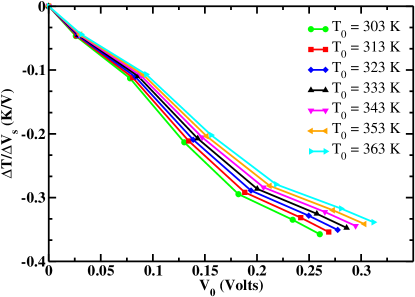
Figure 2: (a) Effects of initial temperature ($T_{0}$) and (b) the bulk salt concentration (so that $\rho_{c,b}=0.6023c_{s}$ (nm)^-3 and $c_{s}$ is in moles per litre (M)) on the electrocaloric effect. The left panel corresponds to $c_{s}=0.1$ M and the right panel corresponds to $T_{0}=303$ K. Parameter for double layer thickness $L_{dl}/a$ is found to be $3,4$ and $6$ for $c_{s}=1.0,0.5$ and $0.1$ M, respectively.

It is found that magnitude of $\Delta T/\Delta V_{s}$ is dependent on the initial temperature and the salt concentration in the bulk. In particular, the magnitude decreases with an increase in the temperature and increases with an increase in the salt concentration. The decrease in the magnitude with an increase in the initial temperature is a direct outcome of an increase in the heat capacity of the double layer with an increase in the applied surface potential, as evident from Figure  1(b). The increase in the magnitude of the electrocaloric effect with an increase in the bulk salt concentration results from a decrease in thickness of the double layer ($L_{dl}$). Furthermore, larger free energy and entropic changes are found with an increase in the bulk salt concentration, as shown in Figure $1$(a) in the Supporting Information. It should be noted that qualitatively the same effects are predicted by the PB and MPB approaches, where the free energy and entropy changes increase as $\sqrt{\rho_{c,b}}$. However, quantitatively, the PB and MPB approaches digress from the numerical results due to errors made in predicting the free energy changes. To demonstrate this point, we have shown a comparison of the free energy changes for the same system, estimated using the PB, MPB and the numerical calculations in Figure  4(a). It is found that the PB approach is off by factors of $10-100$ for $eV_{0}/k_{B}T_{0}>10$. In contrast, the MPB approach corrects for some of the errors made in the PB approach but it still deviates from the numerical results by a factor of $3$.

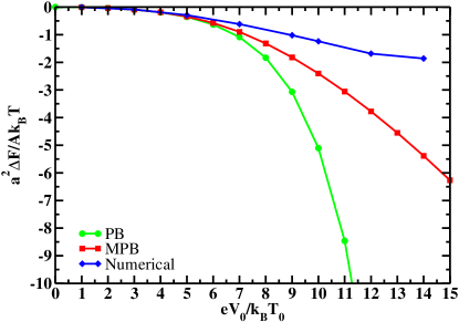
Figure 3: (a) Comparison of the free energy changes computed using the PB approach (i.e., ignoring field-dependent dielectric and steric effects), the MPB approach (i.e., ignoring field-dependent dielectric effects) and the numerical calculations for $c_{s}=0.1$ M, $T_{0}=303$ K. (b) Computed surface charge density as a function of applied surface potential, estimated using the PB, the MPB and the numerical calculations, for different bulk salt concentrations at $T_{0}=303$ K. The solid lines correponds to the analytical relation presented in the text.

The relative importance of the field-dependent dielectric and steric effects in predicting structure of the double layer and resulting changes in the free energy can be assessed by comparing plots showing surface charge density as a function of the surface potential as predicted by the PB, MPB and numerical approaches (Figure  4(b)). The surface charge density in the PB approach is given by $\sigma_{1}=\sigma=\frac{\kappa\epsilon_{h}}{2\pi|Z_{c}|l_{Bo}}\sinh\left[\frac{|Z_{c}|eV_{0}}{2k_{B}T}\right]$ where $|Z_{c}|$ is the valency of ions ($=1$ for monovalent ions), $l_{Bo}=e^{2}/4\pi\epsilon_{0}k_{B}T$ so that $\epsilon_{0}$ is the permittivity of vacuum, $\epsilon_{h}=1+4\pi l_{Bo}p_{s}^{2}\rho_{s,b}/3$ is the relative permittivity of the homogeneous electrolyte solution so that $\rho_{s,b}$ is the solvent density and $\kappa=(8\pi l_{Bo}|Z_{c}|^{2}\rho_{c,b}/\epsilon_{h})^{1/2}$ is the inverse Debye screening length. The PB and MPB approaches predict a monotonic increase in the surface charge density with an increase in the surface potential, as shown in Figure  4(b), without showing any sign of saturation, leading to unphysical surface charge densities. The numerical calculations show agreement with the PB and MPB approaches for $eV_{0}/k_{B}T_{0}<2-4$ depending on the salt concentration and deviate strongly for higher surface potentials exhibiting saturation and a decrease in the surface charge density. This is an outcome of dielectric saturation leading to lowering of dielectric function near the surface, ignored in the PB and MPB approaches. The decrease in the surface charge density with an increase in the surface potential (i.e., negative differential capacitancenegdiff1 ; negdiff2 , where differential capacitance $=\partial\sigma/\partial V_{0}$) hints at the breakdown of the one-dimensional uniform charge density model used here and plausible onset of in-plane charge density wavesnegdiff1 .

In conclusion, we have presented a field theory approach for studying electrocaloric effects in planar double layer systems. Two key ingredients of the theory are the consideration of steric effects and dipolar interactions resulting from polar solvent molecules. Although the theory is general, in this work, we have presented calculations for aqueous solutions containing monovalent salt ions. It was shown that the electrocaloric effect in planar double layer systems is negative, i.e., the temperature of the double layer should decrease with an increase in the applied surface potential. The magnitude of the electrocaloric effect depends on the initial temperature of the solution and the salt concentration. In particular, we showed that the magnitude of the electrocaloric effect should decrease with increase in the initial temperature and increase with an increase in the salt concentration. Due to the general nature of the field theory approachfredbook to tackle curved interfaces, polymers, multivalent ions etc., our work opens up a new area of theoretical research focused on the rational design of electrocaloric fluids. Furthermore, we have shown that the field theory approach stays robust for high surface potentials and the other approaches such as the PB and MPB are not reliable. This particular feature of the field theory is quite important for energy harvesting technologies based on electrochemical capacitors and supercapacitors.

We acknowledge support from the Center for Nanophase Materials Sciences, which is sponsored at Oak Ridge National Laboratory by the Scientific User Facilities Division, office of Basic Energy Sciences, U.S. Department of Energy (DOE).

I Supporting Information: Theory

We consider two parallel plates separated by distance $L$ and immersed in an electrolyte solution containing $n_{s}$ solvent molecules, $n_{+}$ positive and $n_{-}$ negative ions. The plates are assumed to have uniform surface charge densities (number of charges per unit area), $\sigma_{1}$ and $\sigma_{2}$ (in units of electronic charge, $e$) and the corresponding surface potentials are $V_{0,1}$ and $V_{0,2}$, respectively. It is to be noted that surface potentials and charge densities are related to each other by electrostatic boundary conditionsintermolecular_forces and depend on the mechanisms by which the plates acquire the surface charge. These relations can be formally derived by considering different mechanisms for chargingintermolecular_forces .

Molecular volumes of the solvent, positive and negative ions are taken to be $v_{s},v_{+}$ and $v_{-}$, respectively. We are interested in understanding the effects of dipolar interactions and finite ion sizes on the thermodynamics of double layer. For such purposes, we seek a minimal model that can capture the underlying physics. In this work, we have studied a minimal model based on treating each solvent molecule as an electric dipole of length $p_{s}$ occupying molecular volume $v_{s}$. Also, the positive and negative ions have molecular volumes of $v_{+}$ and $v_{-}$, respectively. Finite polarizabilityonsager_moments ; dielectric of ions and solvent molecules are not considered in this work. However, the current formalism can be extended to take into account the effects of polarizability.

The canonical partition function for such a system is writtenorland ; kumar_kilbey as

$$Z = \int\prod_{j=\pm,s}\frac{1}{n_{j}!}\prod_{\alpha=1}^{n_{j}}d\mathbf{r}_{j,\alpha}\int\prod_{\alpha=1}^{n_{s}}d\mathbf{u}_{\alpha}\exp\left[-\hat{H}\left\{\mathbf{r}_{j,\alpha},\mathbf{u}_{\alpha}\right\}\right]\prod_{\mathbf{r}}\mathbf{\delta}\left(\sum_{j=\pm,s}\hat{\rho}_{j}(\mathbf{r})v_{j}-1\right)$$ (1)

where $\mathbf{r}_{j,\alpha}$ is the position vector for the $\alpha^{th}$ particle of type $j$ and $\mathbf{u}_{\alpha}$ is the unit vector quantifying orientation of $\alpha^{th}$ solvent dipole. The Hamiltonian is written by taking into account the contributions coming from ion-ion, ion-dipole and dipole-dipole interactions. Short range interactions between ions and solvent molecules are ignored in the minimal model studied here. $\hat{\rho}_{j}(\mathbf{r})$ represents microscopic number density of the particles of type $j$ at a certain location $\mathbf{r}$ defined as

$$\hat{\rho}_{j}(\mathbf{r}) = \sum_{\alpha=1}^{n_{j}}\delta\left(\mathbf{r}-\mathbf{r}_{j,\alpha}\right)\quad\mbox{for}\quad j=s,+,-$$ (2)

The Hamiltonian for the ions and dipoles can be written asorland ; kumar_kilbey

$$\hat{H} = \frac{l_{Bo}}{2}\int d\mathbf{r}\int d\mathbf{r}^{\prime}\frac{\left[\hat{\rho}_{e}(\mathbf{r})-\nabla_{\mathbf{r}}.\hat{P}(\mathbf{r})\right]\left[\hat{\rho}_{e}(\mathbf{r}^{\prime})-\nabla_{\mathbf{r}^{\prime}}.\hat{P}(\mathbf{r}^{\prime})\right]}{|\mathbf{r}-\mathbf{r}^{\prime}|}$$ (3)

where $l_{Bo}=e^{2}/4\pi\epsilon_{o}k_{B}T$ is the Bjerrum length in vaccum and $\hat{\rho}_{e}(\mathbf{r})$ is the charge density (in units of $e$), given by $\hat{\rho}_{e}(\mathbf{r})=\sum_{j=\pm}Z_{j}\hat{\rho}_{j}(\mathbf{r})+\sigma_{1}\delta(x-x_{1})+\sigma_{2}\delta(x-x_{2})$, $Z_{j}$ being the valency (with sign) of ions of type $j$ and $|x_{2}-x_{1}|=L$ is the distance between the plates. Also, $\hat{P}(\mathbf{r})$ is polarization density of dipoles (in units of $e$) at location $\mathbf{r}$, given by

$$\hat{P}(\mathbf{r}) = p_{s}\sum_{\alpha=1}^{n_{s}}\delta\left(\mathbf{r}-\mathbf{r}_{\alpha}\right)\mathbf{u}_{\alpha}$$ (4)

I.1 Field theory in the canonical ensemble

A field theory for the system described above can be constructed following a standard protocolfredbook . We start from the electrostatics contributions to the partition function. For the electrostatics contribution to the partition function written in the form Eq.  3, we use Hubbard-Stratonovich transformationfredbook so that

$$\exp\left[-\hat{H}\right] = \frac{1}{N_{\psi}}\int D\left[\psi\right]\exp\left[-i\int d\mathbf{r}\left\{\hat{\rho}_{e}(\mathbf{r})-\nabla_{\mathbf{r}}.\hat{P}(\mathbf{r})\right\}\psi(\mathbf{r})+\frac{1}{8\pi l_{Bo}}\int d\mathbf{r}\psi(\mathbf{r})\nabla_{\mathbf{r}}^{2}\psi(\mathbf{r}))\right]$$

where $N_{\psi}$ is a normalization factor, given by

$$N_{\psi} = \int D\left[\psi\right]\exp\left[\frac{1}{8\pi l_{Bo}}\int d\mathbf{r}\psi(\mathbf{r})\nabla_{\mathbf{r}}^{2}\psi(\mathbf{r}))\right]$$ (6)

Using this transformation and writing the local constraints (represented by delta functions) in terms of functional integrals using

$$\prod_{\mathbf{r}}\mathbf{\delta}\left(\sum_{j=\pm,s}\hat{\rho}_{j}(\mathbf{r})v_{j}-1\right) = \int D\left[\eta\right]\exp\left[-i\int d\mathbf{r}\eta(\mathbf{r})\left\{\sum_{j=\pm,s}\hat{\rho}_{j}(\mathbf{r})v_{j}-1\right\}\right]$$ (7)

we can write the partition function given by Eq.  1 as

$$Z = \frac{1}{N_{\psi}}\int D\left[\psi\right]\int D\left[\eta\right]\exp\left[-\frac{H}{k_{B}T}\right]$$ (8)

where

$$\frac{H}{k_{B}T} = -\frac{1}{8\pi l_{Bo}}\int d\mathbf{r}\psi(\mathbf{r})\nabla_{\mathbf{r}}^{2}\psi(\mathbf{r})-i\int d\mathbf{r}\eta(\mathbf{r})+\sigma_{1}\int d\mathbf{r_{\parallel}}i\psi(\mathbf{r_{\parallel}},x_{1})$$ (9)

$$+\sigma_{2}\int d\mathbf{r_{\parallel}}i\psi(\mathbf{r_{\parallel}},x_{2})-\sum_{j=\pm,s}\left\{n_{j}\ln Q_{j}\left\{\psi,\eta\right\}-\ln n_{j}!\right\}$$

and we have used the notation $\mathbf{r}=(x,y,z)\equiv(x,\mathbf{r_{\parallel}})$ so that $\mathbf{r_{\parallel}}$ denotes in-plane vector parallel to the plates. $Q_{j}$ is the partition function for particles of type $j$, given by

$$Q_{j=\pm}\left\{\psi,\eta\right\} = \int d\mathbf{r}\exp\left[-iZ_{j}\psi(\mathbf{r})-iv_{j}\eta(\mathbf{r})\right]$$ (10)

$$Q_{s}\left\{\psi,\eta\right\} = \int d\mathbf{r}\int d\mathbf{u}\exp\left[-ip_{s}\mathbf{u}.\nabla_{\mathbf{r}}\psi(\mathbf{r})-iv_{s}\eta(\mathbf{r})\right]$$ (11)

In the following, we use the saddle-point approximation to estimate the functional integrals over $\psi$ and $\eta$. An equivalent calculation in the grand canonical ensemble is presented in the Appendix A.

I.2 Saddle-point approximation: self-consistent equations, free energy and chemical potentials

The saddle point approximation with respect to $\eta$ and $\psi$ gives two non-linear equations. At the saddle-points, both $\eta$ and $\psi$ turn out to be purely imaginary. Writing $i\eta(\mathbf{r})=\eta^{\star}(\mathbf{r})$ and $i\psi(\mathbf{r})=\psi^{\star}(\mathbf{r})$ at the saddle point and defining densities of ions and solvent molecules via

$$\rho_{j=\pm}(\mathbf{r}) = \frac{n_{j}}{Q_{j}\left\{\psi^{\star},\eta^{\star}\right\}}\exp\left[-Z_{j}\psi^{\star}(\mathbf{r})-v_{j}\eta^{\star}(\mathbf{r})\right]$$ (12)

$$\rho_{s}(\mathbf{r}) = \frac{4\pi n_{s}}{Q_{s}\left\{\psi^{\star},\eta^{\star}\right\}}\exp\left[-v_{s}\eta^{\star}(\mathbf{r})\right]\frac{\sinh p_{s}|\nabla_{\mathbf{r}}\psi^{\star}(\mathbf{r})|}{p_{s}|\nabla_{\mathbf{r}}\psi^{\star}(\mathbf{r})|}$$ (13)

the equations at the saddle point are given by

$$\sum_{j=\pm}v_{j}\rho_{j}(\mathbf{r})+v_{s}\rho_{s}(\mathbf{r}) = 1$$ (14)

$$\nabla_{\mathbf{r}}\cdot\left[\epsilon(\mathbf{r})\nabla_{\mathbf{r}}\psi^{\star}(\mathbf{r})\right] = -4\pi l_{Bo}\rho_{e}(\mathbf{r})$$ (15)

so that the local charge density ($\rho_{e}(\mathbf{r})$) and dielectric function ($\epsilon(\mathbf{r})$) are given by

$$\rho_{e}(\mathbf{r}) = \sum_{j=\pm}Z_{j}\rho_{j}(\mathbf{r})+\sigma_{1}\delta(x-x_{1})+\sigma_{2}\delta(x-x_{2})$$ (16)

$$\epsilon(\mathbf{r}) = 1+4\pi l_{Bo}p_{s}^{2}\rho_{s}(\mathbf{r})\frac{L\left[p_{s}|\nabla_{\mathbf{r}}\psi^{\star}(\mathbf{r})|\right]}{p_{s}|\nabla_{\mathbf{r}}\psi^{\star}(\mathbf{r})|}$$ (17)

where $L(x)=\coth(x)-1/x$ is the Langevin function. Corresponding Helmholtz free energy ($F$) is given by the approximation $F/k_{B}T=-\ln Z\simeq H^{\star}/k_{B}T=F^{\star}/k_{B}T$ so that (cf. Eq.  9)

$$\frac{F^{\star}}{k_{B}T} = \frac{1}{8\pi l_{Bo}}\int d\mathbf{r}\psi^{\star}(\mathbf{r})\nabla_{\mathbf{r}}^{2}\psi^{\star}(\mathbf{r})-\int d\mathbf{r}\eta^{\star}(\mathbf{r})+\sigma_{1}\int d\mathbf{r_{\parallel}}\psi^{\star}(\mathbf{r_{\parallel}},x_{1})$$ (18)

$$+\sigma_{2}\int d\mathbf{r_{\parallel}}\psi^{\star}(\mathbf{r_{\parallel}},x_{2})-\sum_{j=\pm,s}\left\{n_{j}\ln Q_{j}\left\{\psi^{\star},\eta^{\star}\right\}-\ln n_{j}!\right\}$$

Eq.  18 can be rewritten after eliminating $n_{j}$ using Eqs.  14 and  15. Furthermore, using the Stirling approximation $\ln n!\simeq n\ln n-n$, Eq.  18 can be written as

$$\frac{F^{\star}}{k_{B}T} = \int d\mathbf{r}\rho_{e}(\mathbf{r})\psi^{\star}(\mathbf{r})+\frac{1}{8\pi l_{Bo}}\int d\mathbf{r}\psi^{\star}(\mathbf{r})\nabla_{\mathbf{r}}^{2}\psi^{\star}(\mathbf{r})$$ (19)

$$-\int d\mathbf{r}\rho_{s}(\mathbf{r})\ln\left[4\pi\frac{\sinh p_{s}|\nabla_{\mathbf{r}}\psi^{\star}(\mathbf{r})|}{p_{s}|\nabla_{\mathbf{r}}\psi^{\star}(\mathbf{r})|}\right]+\sum_{j=\pm,s}\int d\mathbf{r}\rho_{j}(\mathbf{r})\left[\ln\rho_{j}(\mathbf{r})-1\right]$$

For study of opposing double layer systems in equilibrium with an electrolyte solution, chemical potential is determined by conditions in the solution far from the plates. In order to fix the chemical potentials by specifying different conditions in the solution far from the plates, we rewrite the above equations in terms of chemical potenials. An approximation for the chemical potentials ($\mu_{j}$) of different species can be derived from Eq.  18 using the thermodynamic relation $\mu_{j}=(\partial F/\partial n_{j})_{\Omega}\simeq(\partial F^{\star}/\partial n_{j})_{\Omega}=\mu_{j}^{\star},\Omega$ being the total volume. Using the Stirling approximation $\ln n!\simeq n\ln n-n$, the chemical potentials within the saddle-point approximation are given by

$$\frac{\mu_{j=\pm,s}^{\star}}{k_{B}T} = \ln\left[\frac{n_{j}}{Q_{j}\left\{\psi^{\star},\eta^{\star}\right\}}\right]$$ (20)

Using Eq.  20, Eqs.  12 and  13 can be written as

$$\rho_{j=\pm}(\mathbf{r}) = \exp\left[\frac{\mu_{j}^{\star}}{k_{B}T}-Z_{j}\psi^{\star}(\mathbf{r})-v_{j}\eta^{\star}(\mathbf{r})\right]$$ (21)

$$\rho_{s}(\mathbf{r}) = 4\pi\exp\left[\frac{\mu_{s}^{\star}}{k_{B}T}-v_{s}\eta^{\star}(\mathbf{r})\right]\frac{\sinh p_{s}|\nabla_{\mathbf{r}}\psi^{\star}(\mathbf{r})|}{p_{s}|\nabla_{\mathbf{r}}\psi^{\star}(\mathbf{r})|}$$ (22)

I.3 Chemical part of the free energy: charging the electrodes and adsorption-desorption electrochemical equilibrium

The free energy (cf. Eq.  19) for the two opposing double layer system is obtained for a given surface charge density of the plates and has the charged plates at given surface potentials (in vacuum) as the reference frame. This can be easily seen by putting $\rho_{j=\pm,s}=0$ in Eq.  19 so that $F^{\star}/k_{B}T\left\{\rho_{j=\pm,s}=0\right\}=(\sigma_{1}/2)\int d\mathbf{r_{\parallel}}\psi^{\star}(\mathbf{r_{\parallel}},x_{1})+(\sigma_{2}/2)\int d\mathbf{r_{\parallel}}\psi^{\star}(\mathbf{r_{\parallel}},x_{2})$. This, in turn, means that Eq.  19 doesn’t include the work done (typically by an external source) in charging the two plates at a separation distance of $L=|x_{1}-x_{2}|$. This contributionverweybook ; overbeekPaper to the free energy is

$$\frac{F_{chem}}{k_{B}T} = -\int d\mathbf{r_{\parallel}}\int_{0}^{\sigma_{1}}d\sigma^{\prime}\psi^{\star}(\mathbf{r_{\parallel}},x_{1})\left\{\sigma^{\prime}\right\}-\int d\mathbf{r_{\parallel}}\int_{0}^{\sigma_{2}}d\sigma^{\prime}\psi^{\star}(\mathbf{r_{\parallel}},x_{2})\left\{\sigma^{\prime}\right\}$$ (23)

Evaluation of the right hand side in Eq.  23 requires specification of the mechanisms by which the plates acquire their charge. In the following, we consider the specific case when plates are kept at constant surface potentials.

I.4 One dimensional model: plates at constant surface potentials with symmetrical ions and solvent molecules

If the densities far from the plates are known to be $\rho_{j,b}$ corresponding to spatially uniform $\psi^{\star}(\mathbf{r})=\psi^{\star}_{b}$ and $\eta^{\star}(\mathbf{r})=\eta^{\star}_{b}$ then Eqs.  21 and  22 can be written as

$$\rho_{j=\pm}(\mathbf{r}) = \rho_{j,b}\exp\left[-Z_{j}\left\{\psi^{\star}(\mathbf{r})-\psi^{\star}_{b}\right\}-v_{j}\left\{\eta^{\star}(\mathbf{r})-\eta^{\star}_{b}\right\}\right]$$ (24)

$$\rho_{s}(\mathbf{r}) = \rho_{s,b}\exp\left[-v_{s}\left\{\eta^{\star}(\mathbf{r})-\eta^{\star}_{b}\right\}\right]\frac{\sinh p_{s}|\nabla_{\mathbf{r}}\psi^{\star}(\mathbf{r})|}{p_{s}|\nabla_{\mathbf{r}}\psi^{\star}(\mathbf{r})|}$$ (25)

For two parallel plates, saddle point value of $\psi$ varies only along the direction perpendicular to the charged surface (taken to be along x-axis) so that $\psi^{\star}(\mathbf{r})\equiv\psi^{\star}(x),\eta^{\star}(\mathbf{r})\equiv\eta^{\star}(x)$. Furthermore, considering the case of symmetric ions and solvent molecules so that $v_{j=\pm,s}=a^{3}$ and $Z_{+}=-Z_{-}=|Z_{c}|$ so that $\rho_{j=\pm,b}=\rho_{c,b}$, we can eliminate $\eta^{\star}$ using Eqs.  14,  24 and  25 and write Eq.  15 as

$$\frac{\partial}{\partial x}\left[\epsilon(x)\frac{\partial\psi^{\star}(x)}{\partial x}\right] = -4\pi l_{Bo}\rho_{e}(x)$$ (26)

where the local charge density ($\rho_{e}(x)$) and dielectric function ($\epsilon(x)$) are given by

$$\rho_{e}(x) = |Z_{c}|\left[\rho_{+}(x)-\rho_{-}(x)\right]+\sigma_{1}\delta(x-x_{1})+\sigma_{2}\delta(x-x_{2})$$ (27)

$$\rho_{+}(x) = \frac{\rho_{c,b}\exp\left[-|Z_{c}|\left\{\psi^{\star}(x)-\psi^{\star}_{b}\right\}\right]}{f\left\{\psi^{\star}(x)-\psi^{\star}_{b},\frac{\partial\psi^{\star}(x)}{\partial x}\right\}}$$ (28)

$$\rho_{-}(x) = \frac{\rho_{c,b}\exp\left[|Z_{c}|\left\{\psi^{\star}(x)-\psi^{\star}_{b}\right\}\right]}{f\left\{\psi^{\star}(x)-\psi^{\star}_{b},\frac{\partial\psi^{\star}(x)}{\partial x}\right\}}$$ (29)

$$\epsilon(x) = 1+4\pi l_{Bo}p_{s}^{2}\frac{\rho_{s,b}}{f\left\{\psi^{\star}(x)-\psi^{\star}_{b},\frac{\partial\psi^{\star}(x)}{\partial x}\right\}}\frac{\sinh p_{s}|\frac{\partial\psi^{\star}(x)}{\partial x}|}{p_{s}|\frac{\partial\psi^{\star}(x)}{\partial x}|}\frac{L\left[p_{s}|\frac{\partial\psi^{\star}(x)}{\partial x}|\right]}{p_{s}|\frac{\partial\psi^{\star}(x)}{\partial x}|}$$ (30)

so that

$$f\left\{\psi^{\star}(x)-\psi^{\star}_{b},\frac{\partial\psi^{\star}(x)}{\partial x}\right\} = \rho_{s,b}a^{3}\frac{\sinh p_{s}|\frac{\partial\psi^{\star}(x)}{\partial x}|}{p_{s}|\frac{\partial\psi^{\star}(x)}{\partial x}|}+2\rho_{c,b}a^{3}\cosh\left[|Z_{c}|\left\{\psi^{\star}(x)-\psi^{\star}_{b}\right\}\right]$$ (31)

and $\left[\rho_{s,b}+2\rho_{c,b}\right]a^{3}=1$. It is to be noted that solvent density is given by

$$\rho_{s}(x) = \frac{\rho_{s,b}}{f\left\{\psi^{\star}(x)-\psi^{\star}_{b},\frac{\partial\psi^{\star}(x)}{\partial x}\right\}}\frac{\sinh p_{s}|\frac{\partial\psi^{\star}(x)}{\partial x}|}{p_{s}|\frac{\partial\psi^{\star}(x)}{\partial x}|}$$ (32)

and satisfies the incompressibility constraint $\sum_{j=\pm,s}\rho_{j}(x)a^{3}=1$.

I.5 Free energy within saddle-point approximation : adiabatic changes

Changes in entropy ($\Delta S$) can be readily calculated from the corresponding free energy changes ($\Delta F$) and the thermodynamic relation $\Delta S=-\left(\frac{\partial\Delta F}{\partial T}\right)_{\Omega}$. Free energy of the double layer system ($F^{\star}_{dl}$) is the sum of electrostatic contributions approximated by $F^{\star}$ and the chemical part given by $F_{chem}^{\star}$. Superscript $\star$ implies the use of saddle-point approximation (mean-field like treatment) in estimating the free energy. In particular, assuming lateral homogeneity, for plates (at known surface potentials) separated by distance $L$ having surface area $A$ each, $F^{\star}$ and $F_{chem}^{\star}$ are given by

$$\frac{F^{\star}}{Ak_{B}T} = \int_{0}^{L}dx\rho_{e}(x)\psi^{\star}(x)+\frac{1}{8\pi l_{Bo}}\int_{0}^{L}dx\psi^{\star}(x)\frac{\partial^{2}\psi^{\star}(x)}{\partial x^{2}}$$ (33)

$$-\int_{0}^{L}dx\rho_{s}(x)\ln\left[4\pi\frac{\sinh p_{s}|\frac{\partial\psi^{\star}(x)}{\partial x}|}{p_{s}|\frac{\partial\psi^{\star}(x)}{\partial x}|}\right]+\sum_{j=\pm,s}\int_{0}^{L}dx\rho_{j}(x)\left[\ln\rho_{j}(x)-1\right]$$

and

$$\frac{F_{chem}^{\star}}{Ak_{B}T} = -\sigma_{1}\psi^{\star}(x_{1})-\sigma_{2}\psi^{\star}(x_{2})$$ (34)

In order to compute the electrocaloric effect, free energy changes with respect to the system in the absence of applied electric field are desirable. In the absence of applied electric field (i.e., when $\sigma_{1}=\sigma_{2}=0$ and considered as the reference state), the same number of ions and solvent molecules are homogeneously distributed in volume $\Omega=AL$ so that free energy of the reference state becomes

$$\frac{F_{h}^{\star}}{ALk_{B}T}=\left[\frac{F^{\star}+F_{chem}^{\star}}{ALk_{B}T}\right]_{\sigma_{1}=\sigma_{2}=0} = 2\rho_{c,b}\left[\ln\rho_{c,b}-1\right]+\rho_{s,b}\left[\ln\rho_{s,b}-1-\ln 4\pi\right]$$ (35)

where, we have used the constraint $A\int_{0}^{L}dx\rho_{j,x}=\rho_{j,b}\Omega$ for equating the number of ions and solvent molecules in the absence and presence of applied electric field. Using these equations, the free energy changes ($\Delta F^{\star}$) due to the application of an electric field can be written as

$$\frac{\Delta F^{\star}}{Ak_{B}T}=\frac{F_{dl}^{\star}-F_{h}^{\star}}{Ak_{B}T} = \frac{F^{\star}-F_{h}^{\star}}{Ak_{B}T}-\sigma_{1}\psi^{\star}(x_{1})-\sigma_{2}\psi^{\star}(x_{2})$$ (36)

I.6 Spatially uniform dielectric : Poisson-Boltzmann (PB) and modified Poisson-Boltzmann (MPB) approaches

In the limits of small surface potentials so that $\psi^{\star}(x)-\psi_{b}^{\star}\rightarrow 0$ and weak coupling limt for dipoles, defined by $p_{s}|\frac{\partial\psi^{\star}(x)}{\partial x}|\rightarrow 0$, the dielectric function given by Eq.  30 becomes spatially uniform so that

$$\epsilon(x)\equiv\epsilon_{h} = 1+\frac{4\pi}{3}l_{Bo}p_{s}^{2}\rho_{s,b}$$ (37)

Physically, this means that solvent density is spatially uniform in the limits of small surface potentials and weak coupling limit for dipoles so that $\rho_{s}(x)=\rho_{s,b}$ as evident from Eq.  32. It is to be noted that the quantity $f$ is taken to be unity in these limits and leads to the standard Poisson-Boltzmann results pioneered by Verwey and Overbeekverweybook . Another somewhat recent development (so called modified Poisson-Boltzmann (MPB) approachkornyshev ) is to consider the case of uniform dielectric but include steric effects in the calculations of charge density by taking

$$f\left\{\psi^{\star}(x)-\psi^{\star}_{b},\frac{\partial\psi^{\star}(x)}{\partial x}\right\} \equiv f_{MPB}\left\{\psi^{\star}(x)-\psi^{\star}_{b}\right\}=1-\alpha_{0}+\alpha_{0}\cosh\left[|Z_{c}|\left\{\psi^{\star}(x)-\psi^{\star}_{b}\right\}\right]$$

, where $\alpha_{0}=2\rho_{c,b}a^{3}$ is the packing fraction of ions in the bulk. Although it seems inconsistent to ignore and retain functional dependence of a particular quantity such as $f$ while considering different physical quantities such as dielectric function and charge density, the MPB approach has been quite successful in predicting qualitative features of the double layer capacitance. Nevertheless, the MPB approach leads to semi-analytical predictions for the electrostatic potential and the free energy, as described below.

With the approximations described above, Eq.  26 can be readily integrated over $x$ (after multiplying by $\frac{\partial\psi^{\star}(x)}{\partial x}$ on both sides). In particular, we obtain a self-consistent equation for $\frac{\partial\psi^{\star}(x)}{\partial x}$

$$\frac{1}{2}\left[\frac{\partial\psi^{\star}(x)}{\partial x}\right]^{2} = \frac{4\pi l_{Bo}}{\epsilon_{h}a^{3}}\left[\ln f_{MPB}\left\{\psi^{\star}(x)-\psi^{\star}_{b}\right\}-\lambda\right]$$ (39)

where $\lambda$ is an integration constant, which is determined below and the effects of surface charge densities ($\sigma_{1},\sigma_{2}$) appear in the form of boundary conditions. Using Eq.  39 and equations at the saddle-point, the free energy changes of the double layer system, defined by Eq.  36, can be written as

$$\frac{\Delta F^{\star}_{MPB}}{Ak_{B}T} = \frac{F_{dl,MPB}^{\star}-F_{h}}{Ak_{B}T}=-\frac{\lambda L}{a^{3}}-\frac{2}{a^{3}}\int_{\psi^{\star}(x_{1})}^{\psi^{\star}(x_{2})}d\psi\frac{\left[\ln f_{MPB}\left\{\psi^{\star}(x)-\psi^{\star}_{b}\right\}-\lambda\right]}{\frac{\partial\psi^{\star}(x)}{\partial x}}$$ (40)

where $F_{dl,MPB}=F^{\star}_{MPB}+F_{chem}^{\star}$ and $F^{\star}_{MPB}$ is the approximation for Eq.  33 obtained using Eq.  39 and $F_{chem}^{\star}$ is given by Eq.  34. We must point out that in obtaining Eq.  40, we have retained functional dependence of the solvent density on $f_{MPB}$ through Eq.  32 and used the incompressibility constraint.

In the following, we consider two cases of non-overlapping and overlapping double layers and eliminate $\lambda$ from Eq. 40. In the case of non-overlapping double layers, $\psi^{\star}(x)$ becomes a non-monotonic function of $x$ with a minimum at $x=x_{min}$. Integrating Eq.  39 over $x$ with the limits $x_{1}$ and $x_{2}$, we obtainoverbeekPaper

$$\int_{\psi^{\star}(x_{min})}^{\psi^{\star}(x_{1})}\frac{d\psi^{\star}}{\left[\ln f_{MPB}\left\{\psi^{\star}(x)-\psi^{\star}_{b}\right\}-\lambda\right]^{1/2}}+\int_{\psi^{\star}(x_{min})}^{\psi^{\star}(x_{1})}\frac{d\psi^{\star}}{\left[\ln f_{MPB}\left\{\psi^{\star}(x)-\psi^{\star}_{b}\right\}-\lambda\right]^{1/2}}$$

$$=\left[\frac{8\pi l_{Bo}}{\epsilon_{h}a^{3}}\right]^{1/2}L\quad\quad\quad$$ (41)

Similarly, for the case of overlapping double layers so that $\psi^{\star}(x_{1})>\psi^{\star}(x_{2})$, we obtain

$$\int_{\psi^{\star}(x_{2})}^{\psi^{\star}(x_{1})}\frac{d\psi^{\star}}{\left[\ln f_{MPB}\left\{\psi^{\star}(x)-\psi^{\star}_{b}\right\}-\lambda\right]^{1/2}} = \left[\frac{8\pi l_{Bo}}{\epsilon_{h}a^{3}}\right]^{1/2}L$$ (42)

Eqs.  41 and  42 allows us to eliminate $\lambda$ from Eq.  40 and write it as

$$\frac{\Delta F^{\star}_{MPB}}{Ak_{B}T} = -\sqrt{\frac{\epsilon_{h}}{2\pi l_{Bo}a^{3}}}g\left\{\psi^{\star}(x_{1}),\psi^{\star}(x_{2})\right\}=-\frac{4\rho_{c,b}|Z_{c}|}{\sqrt{2\kappa^{2}\alpha_{o}}}g\left\{\psi^{\star}(x_{1}),\psi^{\star}(x_{2})\right\}$$ (43)

where we have defined $\kappa^{2}=8\pi l_{Bo}|Z_{c}|^{2}\rho_{c,b}/\epsilon_{h}$. Also,

$$g\left\{\psi^{\star}(x_{1}),\psi^{\star}(x_{2})\right\} = \sum_{k=1,2}\int_{\psi^{\star}(x_{min})}^{\psi^{\star}(x_{k})}d\psi\sqrt{\ln f_{MPB}\left\{\psi^{\star}(x)-\psi^{\star}_{b}\right\}}$$ (44)

for the non-overlapping double layers and

$$g\left\{\psi^{\star}(x_{1}),\psi^{\star}(x_{2})\right\} = \int_{\psi^{\star}(x_{2})}^{\psi^{\star}(x_{1})}d\psi\sqrt{\ln f_{MPB}\left\{\psi^{\star}(x)-\psi^{\star}_{b}\right\}}$$ (45)

in the case of overlapping double layers.

Changes in entropy ($\Delta S^{\star}_{MPB}$) can be readily calculated using Eq.  43 and the thermodynamic relation $\Delta S=-\left(\frac{\partial\Delta F}{\partial T}\right)_{\Omega}$ so that

$$\frac{\Delta S^{\star}_{MPB}}{Ak_{B}} = -\left(\frac{\partial\Delta F^{\star}_{MPB}}{Ak_{B}\partial T}\right)_{\Omega}=\frac{6\rho_{c,b}|Z_{c}|}{\sqrt{2\kappa^{2}\alpha_{o}}}g\left[1+\frac{2T}{3g}\frac{\partial g}{\partial T}\right]$$ (46)

where we have dropped explicit functional dependencies of $g$ on $\psi^{\star}(x)-\psi^{\star}_{b}$ for convenience in writing. It is interesting to consider the limit of dilute solutions so that $\alpha_{0}\rightarrow 0$ and this limit is the same as the standard PB approach. In this limit, for non-overlapping double layers, $\psi^{\star}(x_{min})=\psi^{\star}_{b}$ and $\lambda=1$ (due to the fact that $\partial\psi^{\star}(x)/\partial x=0$ at $x=x_{min}$ in Eq.  39). This leads to

$$\frac{\Delta F^{\star}_{PB}}{Ak_{B}T} = \frac{4\rho_{c,b}}{\kappa}\sum_{k=1,2}\left[2-2\cosh\left(|Z_{c}|\left\{\psi^{\star}(x_{k})-\psi^{\star}_{b}\right\}\right)\right]$$ (47)

i.e., the total free energy change is the sum of changes in the individual double layersoverbeekPaper . This leads to entropic changes given by

$$\frac{\Delta S^{\star}_{PB}}{Ak_{B}} = -\frac{4\rho_{c,b}}{\kappa}\sum_{k=1,2}\left[3-2\cosh\left(\frac{|Z_{c}|}{2}\left\{\psi^{\star}(x_{k})-\psi^{\star}_{b}\right\}\right)-\operatorname{sech}\left(\frac{|Z_{c}|}{2}\left\{\psi^{\star}(x_{k})-\psi^{\star}_{b}\right\}\right)\right.$$ (48)

$$\left.+\left\{1-\operatorname{sech}\left(\frac{|Z_{c}|}{2}\left\{\psi^{\star}(x_{k})-\psi^{\star}_{b}\right\}\right)\right\}\frac{T}{\epsilon_{h}}\frac{\partial\epsilon_{h}}{\partial T}\right]$$

II Numerical methods

We have solved the set of equations (Eqs.  26- 32) numerically after rewriting Eq.  26 in the form

$$\frac{\partial\psi^{\star}(x)}{\partial t} = \frac{\partial^{2}\psi^{\star}(x)}{\partial x^{2}}+\frac{1}{\epsilon(x)}\frac{\partial\epsilon(x)}{\partial x}\frac{\partial\psi^{\star}(x)}{\partial x}+\frac{4\pi l_{Bo}}{\epsilon(x)}\rho_{e}(x)$$ (49)

where $t$ is a fictitious time. A steady state solution of Eq.  49 is obtained by using the extrapolated gearkumar_kilbey scheme and using size of ions $a$ to obtain dimensionless length variables. Time step of $0.0001$ is used to integrate Eq.  49 with $L/a=20-40$ (depending on the value of $\rho_{c,b}$) and $1024$ grid points. Convergence of the numerical solution is checked by computing free energy changes between two consecutive time steps and the changes less than $0.0001$ are used to set the tolerance criteria. These equations are solved for non-overlapping double layer systems so that one of the surfaces has the known surface potential while the other is grounded (i.e., surface potential is zero). The temperature is changed by varying $l_{Bo}$ and the free energy changes (in units of $Ak_{B}T/a^{2}$) are computed using Eqs.  33,  34,  35 and  36. In computing the electrocaloric effect, we have made use of the fact that the field variable $\psi^{\star}(x)$ in the theory is the electrostatic potential (in units of $k_{B}T/e$) at location $x$. For example, $\psi^{\star}(0)=eV_{0,1}/k_{B}T$ for the single double layer system studied in this work. Numerical estimates for the surface charge densities we obtained by the relation $\sigma=-[\epsilon(x)/4\pi l_{Bo})(\partial\psi^{\star}(x)/\partial x]_{x=0}$.

III Results: anatomy of the double layer

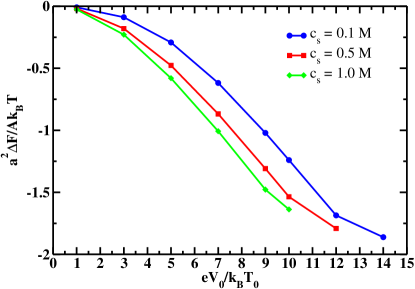
Figure 4: (a) Effects of the bulk salt concentration on the free energy changes ($\Delta F=\Delta F^{\star}$) of the double layer at $T_{0}=303$ K. (b) Comparisons of electrostatic potential profiles ($\psi^{\star}(x)$) from the MPB approach and numerical calculations at $c_{s}=0.1$ M.

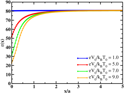
Figure 5: (a) The dielectric function, (b) electrostatic potential, (c) solvent and counterion (anion) densities, and (d) co-ion (cation) densities at different surface potentials are shown for bulk salt concentration of $0.1$ M at $T_{0}=303$ K.

Anatomy of the double layer is determined by the electrostatic potential profile. As the comparisons between the PB and MPB approaches are well-knownkornyshev , we only show comparisons between the MPB and our numerical calculations in Figure  4(b) for low and high surface potentials. It is found that the MPB and numerical results are in excellent agreement at $eV_{0}/k_{B}T_{0}=1$ showing exponential decay appearing as linear on semi-log plot, as expected. In contrast, the electrostatic potential profiles differ near the surface (for $x/a<2$) at $eV_{0}/k_{B}T_{0}=10$, which are responsible for differences in free energies predicted using the MPB approach and the numerical calculations (cf. Figure $3$(a) in the main text).

The differences in the electrostatic potential near the surface show up in plots for surface charge density ($\sigma_{1}=\sigma$) as a function of applied surface potential (Figure $3$(b) in the main text). The structural changes resulting from an increase in the surface potentials are shown in Figure  5. In particular, an increase in surface potentials leads to an increase in the volume fraction of counterions (anions in this case) near the surface at the expense of excluding coions and solvent molecules. However, further increase in the surface potential (e.g., see plot for $eV_{0}/k_{B}T_{0}=9$ in Figure  5(c)) leads to increase in solvent volume fraction near the surface at the expense of exclusion of counterions and coions. This is expected from the expression for solvent volume fraction, Eq.  32, leading to higher volume fraction of solvent in regions having strong electric fields. Also, such an enrichment of solvent in regions of strong electric fields is in agreement with previous theoretical workselectrosorption1 ; electrosorption2 . Furthermore, the electric field dependent sorption of water on the AFM tips has been used to modulate friction at the nanoscaleevgheniFRIC .

APPENDIX A : Field theory for double layer systems in the grand canonical ensemble

For study of a double layer, grand canonical partition function can be constructed and is given by $\Gamma=\sum_{j=\pm,s}e^{\mu_{j}n_{j}/k_{B}T}Z\left\{n_{j}\right\}$ so that

$$\Gamma = \frac{1}{N_{\psi}}\int D\left[\psi\right]\int D\left[\eta\right]\exp\left[-\frac{H_{g}\left\{\psi,\eta\right\}}{k_{B}T}\right]$$ (A-1)

so that

$$\frac{H_{g}\left\{\psi,\eta\right\}}{k_{B}T} = -\frac{1}{8\pi l_{Bo}}\int d\mathbf{r}\psi(\mathbf{r})\nabla_{\mathbf{r}}^{2}\psi(\mathbf{r})-i\int d\mathbf{r}\eta(\mathbf{r})+\sigma_{1}\int d\mathbf{r_{\parallel}}i\psi(\mathbf{r_{\parallel}},x_{1})$$ (A-2)

$$+\sigma_{2}\int d\mathbf{r_{\parallel}}i\psi(\mathbf{r_{\parallel}},x_{2})-\sum_{j=\pm,s}e^{\mu_{j}/k_{B}T}Q_{j}\left\{\psi,\eta\right\}$$

where we have used Eqs.  8 and  9 for the partition function in the canonical ensemble.

The saddle point approximation with respect to $\eta$ and $\psi$ gives two non-linear equations. At the saddle-points, both $\eta$ and $\psi$ turn out to be purely imaginary. Writing $i\eta(\mathbf{r})=\eta^{\star}(\mathbf{r})$ and $i\psi(\mathbf{r})=\psi^{\star}(\mathbf{r})$ at the saddle point, the two equations are given by

$$\sum_{j=\pm}v_{j}\rho_{j}(\mathbf{r})+v_{s}\rho_{s}(\mathbf{r}) = 1$$ (A-3)

$$\nabla_{\mathbf{r}}\cdot\left[\epsilon(\mathbf{r})\nabla_{\mathbf{r}}\psi^{\star}(\mathbf{r})\right] = -4\pi l_{Bo}\rho_{e}(\mathbf{r})$$ (A-4)

where we have defined

$$\rho_{j=\pm}(\mathbf{r}) = \exp\left[\frac{\mu_{j}}{k_{B}T}-Z_{j}\psi^{\star}(\mathbf{r})-v_{j}\eta^{\star}(\mathbf{r})\right]$$ (A-5)

$$\rho_{s}(\mathbf{r}) = 4\pi\exp\left[\frac{\mu_{s}}{k_{B}T}-v_{s}\eta^{\star}(\mathbf{r})\right]\frac{\sinh p_{s}|\nabla_{\mathbf{r}}\psi^{\star}(\mathbf{r})|}{p_{s}|\nabla_{\mathbf{r}}\psi^{\star}(\mathbf{r})|}$$ (A-6)

so that $\rho_{e}(\mathbf{r})=\sum_{j=\pm}Z_{j}\rho_{j}(\mathbf{r})+\sigma_{1}\delta(x-x_{1})+\sigma_{2}\delta(x-x_{2})$ and the local dielectric function is given by

$$\epsilon(\mathbf{r}) = 1+4\pi l_{Bo}p_{s}^{2}\rho_{s}(\mathbf{r})\frac{L\left[p_{s}|\nabla_{\mathbf{r}}\psi^{\star}(\mathbf{r})|\right]}{p_{s}|\nabla_{\mathbf{r}}\psi^{\star}(\mathbf{r})|}$$ (A-7)

where $L(x)=\coth(x)-1/x$ is the Langevin function. Corresponding approximation for the Gibbs free energy is given by

$$\frac{H_{g}^{\star}}{k_{B}T} = \sigma_{1}\int d\mathbf{r_{\parallel}}\psi^{\star}(\mathbf{r_{\parallel}},x_{1})+\sigma_{2}\int d\mathbf{r_{\parallel}}\psi^{\star}(\mathbf{r_{\parallel}},x_{2})+\frac{1}{8\pi l_{Bo}}\int d\mathbf{r}\psi^{\star}(\mathbf{r})\nabla_{\mathbf{r}}^{2}\psi^{\star}(\mathbf{r})$$ (A-8)

$$-\int d\mathbf{r}\eta^{\star}(\mathbf{r})-\sum_{j=\pm,s}\int d\mathbf{r}\rho_{j}(\mathbf{r})$$

Using Eqs.  A-3, A-4,  A-5 and  A-6, it can be shown that $H_{g}^{\star}$ and $F^{\star}$ given by Eq.  19 are related by

$$\frac{F^{\star}}{k_{B}T} = \frac{H_{g}^{\star}}{k_{B}T}+\sum_{j=\pm,s}\frac{\mu_{j}}{k_{B}T}\int d\mathbf{r}\rho_{j}(\mathbf{r})$$ (A-9)

in accordance with the thermodynamic relation that the Helmholtz free energy is the Gibbs free energy plus chemical potential times the number of particles.

REFERENCES

References

• (1) T. Correia, Q. Zhang, Electrocaloric Materials: New Generation of Coolers (Springer, New York, 2014).
• (2) X. Moya, S. Kar-Narayan and N.D. Mathur, Caloric materials near ferroic phase transitions, Nature Materials 13, 439 (2014).
• (3) J.F. Scott, Electrocaloric Materials,Ann. Rev. Mater. Res. 41, 229 (2011).
• (4) L.D. Landau, E.M. Lifshitz and L.P. Pitaevskii, Electrodynamics of Continuous Media (Pergamon Press, New York, 1984).
• (5) W. Thomson, On the thermoelastic, thermomagnetic, and pyroelectric properties of matter, Lond. Edinb. Dublin Phil. Mag. J. Sci. 5, 4 (1878).
• (6) M.E. Lines and A.M. Grass, Principles and Applications of Ferroelectrics and Related Crystals (Clarendon Press, Oxford, UK, 1977).
• (7) B. Neese, B. Chu, S. Lu, Y. Wang, E. Furman, Q. M. Zhang, Large electrocaloric effect in ferroelectric polymers near room temperature, Science 321, 821 (2008).
• (8) X. Qian, S. Lu, X. Li, H. Gu, L. Chien, Q. Zhang, Large electrocaloric effect in a dielectric liquid possessing a large dielectric anisotropy near the isotropic-nematic transition, Adv. Funct. Mater. 23, 2894 (2013).
• (9) C.J.F. Böttcher, Theory of Electric Polarization (Elsevier, Amsterdam, 1973).
• (10) J.P. Hansen and I.R. McDonald, Theory of Simple Liquids (Academic Press, New York, 1976).
• (11) G.H. Fredrickson, The Equilibrium Theory of Inhomogeneous Polymers (Oxford University, New York, 2006).
• (12) R. Kumar, B.G. Sumpter and S.M. Kilbey, Charge regulation and dielectric function in planar polyelectrolyte brushes, J. Chem. Phys. 136, 234901 (2013).
• (13) E.J.W. Verwey, J.Th.G. Overbeek, Theory of the Stability of Lyophobic Colloids (Elsevier, Amsterdam, 1948).
• (14) S. L. Carnie, G. M. Torrie, The statistical mechanics of the electrical double layer, Advances in Chemical Physics 56, 141 (John Wiley and Sons, New York, 1984).
• (15) J.N. Israelachvili, Intermolecular and Surface Forces (Academic Press: San Diego, CA, 1987).
• (16) D.Y.C. Chan, J.J. Mitchel, The free-energy of an electrical double-layer, J. Colloid and Interface Science 95, 193 (1983).
• (17) D. Stigter, K.A. Dill, Free-energy of electrical double-layers - entropy of adsorbed ions and the binding polynomial, J. Phys. Chem. 93, 6737 (1989).
• (18) J.Th.G. Overbeek, The role of energy and entropy in the electrical double layer, Colloids and Surfaces, 51, 61 (1990).
• (19) D. Mccormack, S.L. Carnie, D.Y.C. Chan, Calculations of electrical double-layer force and interaction free-energy between dissimilar surfaces, J. Colloid and Interface Science 169, 177 (1995).
• (20) P.M. Biesheuvel, Electrostatic free energy of interacting ionizable double layers, J. Colloid and Interface Science 275, 514 (2004).
• (21) D.C. Grahame, Effects of dielectric saturation upon the diffuse double layer and the free energy of hydration of ions, J. Chem. Phys. 18, 903 (1950).
• (22) D.C. Grahame, Diffuse double layer theory for electrolytes of unsymmetrical valence types, J. Chem. Phys. 21, 1054 (1953).
• (23) A. Abrashkin, D. Andelman, H. Orland, Dipolar Poisson-Boltzmann equation: Ions and dipoles close to charge interfaces, Phys. Rev. Lett. 99, 077801 (2007).
• (24) M.M. Hatlo, R. Roij, L. Lue, The electric double layer at high surface potentials: The influence of excess ion polarizability, E. Phys. Lett. 97, 28010 (2012).
• (25) A. Levy, D. Andelman, H. Orland, Dipolar Poisson-Boltzmann approach to ionic solutions: A mean field and loop expansion analysis, J. Chem. Phys. 139, 164909 (2013).
• (26) Y. Nakayama, D. Andelman, Differential capacitance of the electric double layer: The interplay between ion finite size and dielectric decrement, J. Chem. Phys. 142, 044706 (2015).
• (27) I. Borukhov, D. Andelman, H. Orland, Steric effects in electrolytes: A modified Poisson-Boltzmann equation, Phys. Rev. Lett. 79, 435 (1997).
• (28) A.A. Kornyshev, Double-Layer in ionic liquids:  paradigm change?, J. Phys. Chem. B 111, 5545 (2007).
• (29) M.Z. Bazant, B.D. Storey, A.A. Kornyshev, Double Layer in ionic liquids: overscreening versus crowding, Phys. Rev. Lett. 106, 046102 (2011).
• (30) M.V. Fedorov, A.A. Kornyshev, Ionic liquids at electrified interfaces, Chemical Reviews 114, 2978 (2014).
• (31) B.W. Ninham, V.A. Parsegian, Electrostatic potential between surfaces bearing ionizable groups in ionic equilibrium with physiologic saline solution, J. Theor. Bio. 31, 405 (1971).
• (32) R. Wang, Z.G. Wang, Continuous self-energy of ions at the dielectric interface, Phys. Rev. Lett. 112, 136101 (2014).
• (33) D. Brogioli, Extracting renewable energy from a salinity difference using a capacitor,Phys. Rev. Lett. 103, 058501 (2009).
• (34) M. Janssen, A. Härtel, R. Roij, Boosting capacitive blue-energy and desalination devices with waste heat, Phys. Rev. Lett. 113, 268501 (2014).
• (35) M.B. Partenskii, P.C. Jordan, Limitations and strengths of uniformly charged double-layer theory: physical significance of capacitance anomalies, Phys. Rev. E 77, 061117 (2008).
• (36) A.I. Khan, K. Chatterjee, B. Wang, S. Drapcho, L. You, C. Serrao, S.R. Bakaul, R. Ramesh, S. Salahuddin, Negative capacitance in a ferroelectric capacitor, Nature Materials 14, 182 (2015).

REFERENCES

• (1) J.N. Israelachvili, Intermolecular and Surface Forces (Academic Press: San Diego, CA, 1987).
• (2) L. Onsager, Journal of Chemical Physics 58, 1486-1493 (1936).
• (3) C.J.F. Böttcher, Theory of Electric Polarization (Elsevier, Amsterdam, 1973).
• (4) A. Abrashkin, D. Andelman, H. Orland, Dipolar Poisson-Boltzmann equation: Ions and dipoles close to charge interfaces, Phys. Rev. Lett. 99, 077801 (2007).
• (5) R. Kumar, B.G. Sumpter and S.M. Kilbey, Charge regulation and dielectric function in planar polyelectrolyte brushes, J. Chem. Phys. 136, 234901 (2013).
• (6) G.H. Fredrickson, The Equilibrium Theory of Inhomogeneous Polymers (Oxford University, New York, 2006).
• (7) E.J.W. Verwey, J.Th.G. Overbeek, Theory of the Stability of Lyophobic Colloids (Elsevier, Amsterdam, 1948).
• (8) J.Th.G. Overbeek, The role of energy and entropy in the electrical double layer, Colloids and Surfaces, 51, 61 (1990).
• (9) A.A. Kornyshev, Double-Layer in ionic liquids:  paradigm change?, J. Phys. Chem. B 111, 5545 (2007).
• (10) H.J. Butt, M.B. Untch, A. Golriz, S.A. Pihan, R. Berger, Electric-field-induced condensation: An extension of the Kelvin equation, Phys. Rev. E 83, 061604 (2011).
• (11) G. Feng, X.K. Jiang, R. Qiao, A.A. Kornyshev, Water in ionic liquids at electrified interfaces: The anatomy of electrosorption, ACS Nano 8, 11685 (2014).
• (12) E. Strelcov, R. Kumar, V. Bocharova, B. G. Sumpter, A. Tselev, S. V. Kalinin, Nanoscale lubrication of ionic surfaces controlled via a strong electric field, Scientific Reports 5, 8049 (2015).