Natural Standard Model Alignment in the Two Higgs Doublet Model

Abstract

The current LHC Higgs data provide strong constraints on possible deviations of the couplings of the observed 125 GeV Higgs boson from the Standard Model (SM) expectations. Therefore, it now becomes compelling that any extended Higgs sector must comply with the so-called SM alignment limit. In the context of the Two Higgs Doublet Model (2HDM), this alignment is often associated with either decoupling of the heavy Higgs sector or accidental cancellations in the 2HDM potential. Here we present a new solution realizing natural alignment based on symmetries, without decoupling or fine-tuning. In particular, we show that in 2HDMs where both Higgs doublets acquire vacuum expectation values, there exist only three different symmetry realizations leading to natural alignment. We discuss some phenomenological implications of the Maximally-Symmetric 2HDM based on SO(5) symmetry group and analyze new collider signals for the heavy Higgs sector, involving third-generation quarks, which can be a useful observational tool during the Run-II phase of the LHC.

MAN/HEP/2015/04

1 Introduction

The discovery of a Higgs boson with mass around 125 GeV [1] is the main highlight of the Run-I phase of the LHC, as it provides the first experimental evidence of the Higgs mechanism [2]. Although the measured couplings of the discovered Higgs boson show remarkable compatibility with those predicted by the Standard Model (SM) [3], the current experimental data still leave open the possibility of an extended Higgs sector. In fact, several well-motivated new-physics scenarios necessarily come with an enlarged Higgs sector, such as supersymmetry [4] and axion models [5], in order to address a number of theoretical and cosmological issues, including the gauge hierarchy problem, the origin of the Dark Matter (DM) and matter-antimatter asymmetry in our Universe. Here we consider the simplest extension of the standard Higgs mechanism, namely the Two Higgs Doublet Model (2HDM) [6], where the SM Higgs doublet is supplemented by another isodoublet with hypercharge $Y=1$. This model can provide new sources of spontaneous [7] or explicit [8] CP violation, viable DM candidates [9] and a strong first order phase transition for electroweak baryogenesis [10].

In the doublet field space $\Phi_{1,2}$, where $\Phi_{i}=(\phi_{i}^{+},\phi_{i}^{0})^{\sf T}$, the general 2HDM potential reads

$$V\ =\ -\mu_{1}^{2}(\Phi_{1}^{\dagger}\Phi_{1})-\mu_{2}^{2}(\Phi_{2}^{\dagger}\Phi_{2})-\left[m_{12}^{2}(\Phi_{1}^{\dagger}\Phi_{2})+{\rm H.c.}\right]$$

$$+\lambda_{1}(\Phi_{1}^{\dagger}\Phi_{1})^{2}+\lambda_{2}(\Phi_{2}^{\dagger}\Phi_{2})^{2}+\lambda_{3}(\Phi_{1}^{\dagger}\Phi_{1})(\Phi_{2}^{\dagger}\Phi_{2})+\lambda_{4}(\Phi_{1}^{\dagger}\Phi_{2})(\Phi_{2}^{\dagger}\Phi_{1})$$

$$+\left[\frac{\lambda_{5}}{2}(\Phi_{1}^{\dagger}\Phi_{2})^{2}+\lambda_{6}(\Phi_{1}^{\dagger}\Phi_{1})(\Phi_{1}^{\dagger}\Phi_{2})+\lambda_{7}(\Phi_{1}^{\dagger}\Phi_{2})(\Phi_{2}^{\dagger}\Phi_{2})+{\rm H.c.}\right],$$ (1)

which contains four real mass parameters $\mu_{1,2}^{2}$, Re$(m^{2}_{12})$, Im$(m^{2}_{12})$, and ten real quartic couplings $\lambda_{1,2,3,4}$, Re($\lambda_{5,6,7})$, and Im($\lambda_{5,6,7}$). Thus, the vacuum structure of the general 2HDM can be quite rich [11], as compared to the SM.

The quark-sector Yukawa Lagrangian in the general 2HDM is given by

$$-{\cal L}^{q}_{Y}\ =\ \bar{Q}_{L}(h_{1}^{u}\Phi_{1}+h_{2}^{u}\Phi_{2})u_{R}\>+\>\bar{Q}_{L}(h_{1}^{d}\widetilde{\Phi}_{1}+h_{2}^{d}\widetilde{\Phi}_{2})d_{R}\;,$$ (2)

where $\widetilde{\Phi}_{i}={\rm i}\sigma_{2}\Phi_{i}^{*}$ are the isospin conjugates of $\Phi_{i}$, $Q_{L}=(u_{L},d_{L})^{\sf T}$ is the $SU(2)_{L}$ quark doublet and $u_{R},d_{R}$ are right-handed quark singlets. Due to the Yukawa interactions in (2), the neutral scalar bosons often induce unacceptably large flavor-changing neutral current (FCNC) processes at the tree level. This is usually avoided by imposing a discrete $Z_{2}$ symmetry [12] under which

$$\Phi_{1}\to-\Phi_{1},\quad\Phi_{2}\to\Phi_{2},\quad u_{Ra}\to u_{Ra},\quad d_{Ra}\to d_{Ra}~{}~{}{\rm or}~{}~{}d_{Ra}\to-d_{Ra}\;,$$ (3)

($a=1,2,3$ being the quark family index) so that only $\Phi_{2}$ gives mass to up-quarks, and only $\Phi_{1}$ or only $\Phi_{2}$ gives mass to down-quarks. In this case, the scalar boson couplings to quarks are proportional to the quark mass matrix, as in the SM, and therefore, there is no tree-level FCNC process. The $Z_{2}$ symmetry (3) is satisfied by four discrete choices of tree-level Yukawa couplings between the Higgs doublets and SM fermions, which are known as Type I, II, X (lepton-specific) and Y (flipped) 2HDMs [6]. In Type II, X and Y 2HDM, both Higgs doublets $\Phi_{1,2}$ acquire vacuum expectation values (VEVs) $v_{1,2}$, whereas in Type I 2HDM, one of the Higgs doublets ($\Phi_{1}$) does not couple to the SM fermions and need not acquire a VEV [13]. Global fits to the current LHC Higgs data [14, 15, 16] suggest that all four types of discrete 2HDM are constrained to lie close to the so-called SM alignment limit, where the mass eigenbasis of the CP-even scalar sector aligns with the SM gauge eigenbasis.

Naively, the SM alignment is often associated with the decoupling limit, in which all the non-standard Higgs bosons are assumed to be much heavier than the electroweak scale so that the lightest CP-even scalar behaves just like the SM Higgs boson. This SM alignment limit can also be achieved, without decoupling [17, 18, 19, 20, 21, 22]. However, for small $\tan\beta$ values, this is usually attributed to accidental cancellations in the 2HDM potential [21]. Here we present a symmetry argument to naturally justify the alignment limit [23], independently of the kinematic parameters of the theory, such as the heavy Higgs masses and the ratio of the VEVs ($v_{2}/v_{1}$). In the 2HDMs where both Higgs doublets acquire VEVs, we show that there exist only three possible symmetry realizations of the scalar potential having natural alignment. We explicitly analyze the simplest case, namely the maximally symmetric 2HDM (MS-2HDM) with SO(5) symmetry. We show that the renormalization group (RG) effects due to the hypercharge gauge coupling $g^{\prime}$ and third-generation Yukawa couplings, as well as soft-breaking mass parameters, induce relevant deviations from the SO(5) limit, which lead to distinct predictions for the Higgs spectrum of the MS-2HDM. In particular, the heavy Higgs sector is predicted to be quasi-degenerate, which is a distinct feature of the SO(5) limit, apart from being gaugephobic, which is a generic feature in the alignment limit. Moreover, the current experimental constraints force the heavy Higgs sector to lie above the top-quark threshold in the MS-2HDM. Thus, the dominant collider signal for this sector involves final states with third-generation quarks. We study some of these collider signals for the upcoming run of the LHC.

The plan of this proceedings is as follows: In Section 2, we present the natural alignment condition for a generic 2HDM scalar potential. In Section 3, we list the symmetry classifications of the 2HDM potential and identify the symmetries leading to a natural alignment. In Section 4, we analyze the MS-2HDM in presence of custodial symmetry and soft breaking effects. In Section 5, we discuss some collider phenomenology of the heavy Higgs sector in the alignment limit, with particular emphasis on the heavy Higgs sector beyond the top-quark threshold. Our conclusions are given in Section 6.

2 Natural Alignment Condition

For simplicity, we will consider the 2HDM potential (1) with CP-conserving vacua; the results derived in this section can be easily generalized to the CP-violating 2HDM potential. We start with the linear decomposition of the two Higgs doublets in terms of eight real scalar fields:

$$\Phi_{j}\ =\ \left(\begin{array}[]{c}\phi_{j}^{+}\\ \frac{1}{\sqrt{2}}(v_{j}+\phi_{j}+ia_{j})\end{array}\right)\;,$$ (6)

where $v=\sqrt{v_{1}^{2}+v_{2}^{2}}=246.2$ GeV is the SM electroweak VEV. After symmetry breaking, the three Goldstone modes ($G^{\pm},G^{0}$) become the longitudinal components of the $W^{\pm}$ and $Z$ bosons, and there remain five physical scalar mass eigenstates: two CP-even ($h,H$), one CP-odd ($a$) and two charged ($h^{\pm}$) scalars. The corresponding physical mass eigenvalues are given by [24, 25]

$$M^{2}_{h^{\pm}}\ =\ \frac{m_{12}^{2}}{s_{\beta}c_{\beta}}-\frac{v^{2}}{2}\left(\lambda_{4}+\lambda_{5}\right)+\frac{v^{2}}{2s_{\beta}c_{\beta}}\left(\lambda_{6}c_{\beta}^{2}+\lambda_{7}s_{\beta}^{2}\right),$$ (7a)

$$M_{a}^{2}\ =\ M^{2}_{h^{\pm}}+\frac{v^{2}}{2}\left(\lambda_{4}-\lambda_{5}\right),$$ (7b)

$$M_{H}^{2}\ =\ \frac{1}{2}\left[(A+B)-\sqrt{(A-B)^{2}+4C^{2}}\right],$$ (7c)

$$M_{h}^{2}\ =\ \frac{1}{2}\left[(A+B)+\sqrt{(A-B)^{2}+4C^{2}}\right],$$ (7d)

where we have used the short-hand notations $c_{\beta}\equiv\cos\beta$ and $s_{\beta}\equiv\sin\beta$ with $\tan\beta=v_{2}/v_{1}$, and

$$A\ =\ M_{a}^{2}s_{\beta}^{2}+v^{2}\left(2\lambda_{1}c_{\beta}^{2}+\lambda_{5}s^{2}_{\beta}+2\lambda_{6}s_{\beta}c_{\beta}\right),$$ (8a)

$$B\ =\ M_{a}^{2}c_{\beta}^{2}+v^{2}\left(2\lambda_{2}s_{\beta}^{2}+\lambda_{5}c^{2}_{\beta}+2\lambda_{7}s_{\beta}c_{\beta}\right),$$ (8b)

$$C\ =\ -M_{a}^{2}s_{\beta}c_{\beta}+v^{2}\left(\lambda_{34}s_{\beta}c_{\beta}+\lambda_{6}c^{2}_{\beta}+\lambda_{7}s^{2}_{\beta}\right).$$ (8c)

with $\lambda_{34}=\lambda_{3}+\lambda_{4}$. The mixing between the mass eigenstates in the CP-odd and charged sectors is governed by the angle $\beta$, whereas in the CP-even sector, it is governed by the angle $\alpha$, where $\tan{2\alpha}=2C/(A-B)$.

The SM Higgs field can be identified as the linear combination

$$H_{\rm SM}\ =\ \phi_{1}\cos\beta+\phi_{2}\sin\beta\ =\ H\cos(\beta-\alpha)+h\sin(\beta-\alpha)\;.$$ (9)

From (9), we see that the couplings of $h$ and $H$ to the gauge bosons ($V=W^{\pm},Z$) with respect to the SM Higgs couplings $g_{H_{\rm SM}VV}$ will be

$$g_{hVV}\ =\ \sin{(\beta-\alpha)}\;,\qquad g_{HVV}\ =\ \cos{(\beta-\alpha)}\;.$$ (10)

Thus, the SM alignment limit is defined as the limit $\alpha\to\beta$ (or $\alpha\to\beta-\pi/2$) when $H$ ($h$) couples to the vector bosons exactly like in the SM, whereas $h$ ($H$) becomes gaugephobic. For notational clarity, we will take the alignment limit to be $\alpha\to\beta$ in the following.

To derive the alignment condition, we rewrite the CP-even scalar mass matrix as

$$M^{2}_{S}\ =\ \left(\begin{array}[]{cc}A&C\\ C&B\end{array}\right)\ =\ \left(\begin{array}[]{cc}c_{\beta}&-s_{\beta}\\ s_{\beta}&c_{\beta}\end{array}\right)\left(\begin{array}[]{cc}\widehat{A}&\widehat{C}\\ \widehat{C}&\widehat{B}\end{array}\right)\left(\begin{array}[]{cc}c_{\beta}&s_{\beta}\\ -s_{\beta}&c_{\beta}\end{array}\right)\;,$$ (19)

where

$$\widehat{A} =2v^{2}\Big{[}c_{\beta}^{4}\lambda_{1}+s_{\beta}^{2}c_{\beta}^{2}\lambda_{345}+s_{\beta}^{4}\lambda_{2}\>+\>2s_{\beta}c_{\beta}\Big{(}c^{2}_{\beta}\lambda_{6}+s^{2}_{\beta}\lambda_{7}\Big{)}\Big{]}\;,$$ (20a)

$$\widehat{B} =M_{a}^{2}\>+\>\lambda_{5}v^{2}\>+\>2v^{2}\Big{[}s^{2}_{\beta}c^{2}_{\beta}\Big{(}\lambda_{1}+\lambda_{2}-\lambda_{345}\Big{)}\>-\>s_{\beta}c_{\beta}\Big{(}c^{2}_{\beta}-s^{2}_{\beta}\Big{)}\Big{(}\lambda_{6}-\lambda_{7}\Big{)}\Big{]}\;,$$ (20b)

$$\widehat{C} =v^{2}\Big{[}s^{3}_{\beta}c_{\beta}\Big{(}2\lambda_{2}-\lambda_{345}\Big{)}-c^{3}_{\beta}s_{\beta}\Big{(}2\lambda_{1}-\lambda_{345}\Big{)}+c^{2}_{\beta}\Big{(}1-4s^{2}_{\beta}\Big{)}\lambda_{6}+s^{2}_{\beta}\Big{(}4c^{2}_{\beta}-1\Big{)}\lambda_{7}\Big{]}.$$ (20c)

Here we have used the short-hand notation: $\lambda_{345}\equiv\lambda_{3}+\lambda_{4}+\lambda_{5}$. Evidently, the SM alignment limit $\alpha\to\beta$ is obtained when $\widehat{C}=0$ in (19) [18]. From (20c), this yields the quartic equation

$$\lambda_{7}t_{\beta}^{4}-(2\lambda_{2}-\lambda_{345})t_{\beta}^{3}+3(\lambda_{6}-\lambda_{7})t_{\beta}^{2}+(2\lambda_{1}-\lambda_{345})t_{\beta}-\lambda_{6}\ =\ 0\;.$$ (21)

For natural alignment, (21) should be satisfied for any value of $\tan\beta$, which requires the coefficients of the polynomial in $\tan\beta$ to vanish identically. Imposing this restriction, we arrive at the natural alignment condition [23]

$$2\lambda_{1}\ =\ 2\lambda_{2}\ =\ \lambda_{345}\;,\qquad\lambda_{6}\ =\ \lambda_{7}\ =\ 0\;.$$ (22)

In particular, for $\lambda_{6}=\lambda_{7}=0$ as in the $Z_{2}$-symmetric 2HDMs, (21) has a solution

$$\tan^{2}\beta\ =\ \frac{2\lambda_{1}-\lambda_{345}}{2\lambda_{2}-\lambda_{345}}\ >\ 0\;,$$ (23)

independent of $M_{a}$. After some algebra, the simple solution (23) to our general alignment condition (21) can be shown to be equivalent to that derived in [21, 26].

3 Symmetry Classifications of the 2HDM Potential

The general 2HDM potential (1) may exhibit three different classes of accidental symmetries. The first class of symmetries pertains to transformations of the Higgs doublets $\Phi_{1,2}$ only, but not their complex conjugates $\Phi_{1,2}^{*}$, and are known as the Higgs family (HF) symmetries [19, 27]. The second class of symmetry transformations relates the fields $\Phi_{1,2}$ to their complex conjugates $\Phi_{1,2}^{*}$ and are generically termed as CP symmetries [27]. The third class of symmetries utilize mixed HF and CP transformations that leave the $SU(2)_{L}$ gauge kinetic terms of $\Phi_{1,2}$ canonical [11].

To identify all accidental symmetries of the 2HDM potential, it is convenient to work in the bilinear scalar field formalism [28] by introducing an 8-dimensional complex multiplet [11, 29, 30]:

$${\bf\Phi}\ \equiv\ \left(\begin{array}[]{c}\Phi_{1}\\ \Phi_{2}\\ \widetilde{\Phi}_{1}\\ \widetilde{\Phi}_{2}\end{array}\right)\;,$$ (24)

where $\widetilde{\Phi}_{i}={\rm i}\sigma^{2}\Phi^{*}_{i}$ (with $i=1,2$) and $\sigma^{2}$ is the second Pauli matrix. In terms of the ${\bf\Phi}$-multiplet, the following null 6-dimensional Lorentz vector can be defined [11, 30]:

$$R^{A}\ \equiv\ {\bf\Phi}^{\dagger}\Sigma^{A}{\bf\Phi}\;,$$ (25)

where $A=0,1,...,5$ and the six $8\times 8$-dimensional matrices $\Sigma^{A}$ may be expressed in terms of the three Pauli matrices $\sigma^{1,2,3}$ and the identity matrix $\bm{1}_{2\times 2}\equiv\sigma^{0}$, as follows:

$$\Sigma^{0,1,3}\ =\ \frac{1}{2}\sigma^{0}\otimes\sigma^{0,1,3}\otimes\sigma^{0},\quad\Sigma^{2}\ =\ \frac{1}{2}\sigma^{3}\otimes\sigma^{2}\otimes\sigma^{0},$$

$$\Sigma^{4}\ =\ -\frac{1}{2}\sigma^{2}\otimes\sigma^{2}\otimes\sigma^{0},\quad\Sigma^{5}\ =\ -\frac{1}{2}\sigma^{1}\otimes\sigma^{2}\otimes\sigma^{0}.$$ (26)

Note that the bilinear field space spanned by the 6-vector $R^{A}$ realizes an orthochronous ${\rm SO}(1,5)$ symmetry group.

In terms of the null-vector $R^{A}$ defined in (25), the 2HDM potential (1) takes on a simple quadratic form:

$$V\ =\ -\,\frac{1}{2}\,M_{A}\,R^{A}\>+\>\frac{1}{4}\,L_{AB}\,R^{A}R^{B}\;,$$ (27)

where $M_{A}$ and $L_{AB}$ are ${\rm SO}(1,5)$ constant ‘tensors’ that depend on the mass parameters and quartic couplings given in (1) and their explicit forms may be found in [30, 31]. Requiring that the SU(2)_L gauge-kinetic term of the $\Phi$-multiplet remains canonical restricts the allowed set of rotations from SO(1,5) to SO(5), where only the spatial components $R^{I}$ (with $I=1,...,5$) transform and the zeroth component $R^{0}$ remains invariant. Consequently, in the absence of the hypercharge gauge coupling and fermion Yukawa couplings, the maximal symmetry group of the 2HDM is $G^{R}_{\rm 2HDM}={\rm SO(5)}$. Including all its proper, improper and semi-simple subgroups of SO(5), all accidental symmetries for the 2HDM potential were classified in [11, 30], as shown in Table 1. Here we have used a diagonally reduced basis [32], where ${\rm Im}(\lambda_{5})=0$ and $\lambda_{6}=\lambda_{7}$, thus reducing the number of independent quartic couplings to seven. Each of the symmetries listed in Table 1 leads to certain constraints on the mass and/or coupling parameters.

symmetry	$\mu_{1}^{2}$	$\mu_{2}^{2}$	$m^{2}_{12}$	$\lambda_{1}$	$\lambda_{2}$	$\lambda_{3}$	$\lambda_{4}$	${\rm Re}(\lambda_{5})$	$\lambda_{6}=\lambda_{7}$
$Z_{2}\times$ O(2)	-	-	Real	-	-	-	-	-	Real
$(Z_{2})^{2}\times$SO(2)	-	-	0	-	-	-	-	-	0
$(Z_{2})^{3}\times$O(2)	-	$\mu_{1}^{2}$	0	-	$\lambda_{1}$	-	-	-	0
O(2) $\times$O(2)	-	-	0	-	-	-	-	0	0
$Z_{2}\times$ [O(2)]2	-	$\mu_{1}^{2}$	0	-	$\lambda_{1}$	-	-	$2\lambda_{1}-\lambda_{34}$	0
O(3)$\times$O(2)	-	$\mu_{1}^{2}$	0	-	$\lambda_{1}$	-	$2\lambda_{1}-\lambda_{3}$	0	0
SO(3)	-	-	Real	-	-	-	-	$\lambda_{4}$	Real
$Z_{2}\times$O(3)	-	$\mu_{1}^{2}$	Real	-	$\lambda_{1}$	-	-	$\lambda_{4}$	Real
$(Z_{2})^{2}\times$SO(3)	-	$\mu_{1}^{2}$	0	-	$\lambda_{1}$	-	-	$\pm\lambda_{4}$	0
O(2)$\times$O(3)	-	$\mu_{1}^{2}$	0	-	$\lambda_{1}$	$2\lambda_{1}$	-	0	0
SO(4)	-	-	0	-	-	-	0	0	0
$Z_{2}\times$O(4)	-	$\mu_{1}^{2}$	0	-	$\lambda_{1}$	-	0	0	0
SO(5)	-	$\mu_{1}^{2}$	0	-	$\lambda_{1}$	$2\lambda_{1}$	0	0	0

Table 1: Relations between the parameters of the $U(1)_{Y}$-invariant 2HDM potential (1) for the 13 accidental symmetries [30] in a diagonally reduced basis, where ${\rm Im}(\lambda_{5})=0$ and $\lambda_{6}=\lambda_{7}$. A dash signifies the absence of a constraint for that parameter. Notice that all symmetries lead to a CP-conserving 2HDM potential.

From Table 1, we observe that there are only three symmetries, namely (i) $Z_{2}\times[{\rm O(2)}]^{2}$, (ii) O(3)$\times$ O(2) and (iii) SO(5), which satisfy the natural alignment condition given by (22). Note that in all the three naturally aligned scenarios, $\tan\beta$ as given in (23) ‘consistently’ gives an indefinite answer 0/0. In what follows, we focus on the simplest realization of the SM alignment, namely, the MS-2HDM based on the SO(5) group [23]. A detailed study of the other two cases will be presented elsewhere.

4 Maximally Symmetric 2HDM

From Table 1, we see that the maximal symmetry group in the bilinear field space is SO(5), in which case the parameters of the 2HDM potential (1) satisfy the following relations:

$$\mu_{1}^{2}\ =\ \mu_{2}^{2}\;,\quad m^{2}_{12}\ =\ 0\;,\quad$$

$$\lambda_{2}\ =\ \lambda_{1}\;,\quad\lambda_{3}\ =\ 2\lambda_{1}\;,\quad\lambda_{4}\ =\ {\rm Re}(\lambda_{5})\ =\ \lambda_{6}\ =\ \lambda_{7}\ =\ 0\;,$$ (28)

Thus, in this case, the 2HDM potential (1) is parametrized by just a single mass parameter $\mu_{1}^{2}=\mu_{2}^{2}\equiv\mu^{2}$ and a single quartic coupling $\lambda_{1}=\lambda_{2}=\lambda_{3}/2\equiv\lambda$, as in the SM:

$$V\ =\ -\,\mu^{2}\,\Big{(}|\Phi_{1}|^{2}+|\Phi_{2}|^{2}\Big{)}\>+\>\lambda\,\Big{(}|\Phi_{1}|^{2}+|\Phi_{2}|^{2}\Big{)}^{2}\ =\ -\>\frac{\mu^{2}}{2}\,{\bf\Phi}^{\dagger}\,{\bf\Phi}\ +\ \frac{\lambda}{4}\,\big{(}{\bf\Phi}^{\dagger}\,{\bf\Phi}\big{)}^{2}\;.$$ (29)

Note that the MS-2HDM scalar potential in (29) is more minimal than the respective potential of the MSSM at the tree level. Even in the custodial symmetric limit $g^{\prime}\to 0$, the latter possesses a smaller symmetry: ${\rm O}(2)\times{\rm O}(3)\subset{\rm SO}(5)$, in the 5-dimensional bilinear $R^{I}$ space.

Given the isomorphism of the Lie algebras ${\rm SO(5)}\sim{\rm Sp}(4)$, the maximal symmetry group of the 2HDM in the original $\Phi$-field space is ${\rm G}^{\bf\Phi}_{\rm 2HDM}=\left[{\rm Sp}(4)/Z_{2}\right]\times{\rm SU(2)}_{L}$ [30, 23] in the custodial symmetry limit of vanishing $g^{\prime}$ and fermion Yukawa couplings. We can generalize this result to deduce that in the custodial symmetry limit, the maximal symmetry group for an $n$ Higgs Doublet Model ($n$HDM) will be ${\rm G}^{\bf\Phi}_{n{\rm HDM}}=\left[{\rm Sp}(2n)/Z_{2}\right]\times{\rm SU(2)}_{L}$.

4.1 Scalar Spectrum in the MS-2HDM

Using the parameter relations given by (28), we find from (7a)-(7d) that in the MS-2HDM, the CP-even Higgs $H$ has mass $M_{H}^{2}=2\lambda_{2}v^{2}$, whilst the remaining four scalar fields, denoted hereafter as $h$, $a$ and $h^{\pm}$, are massless. This is a consequence of the Goldstone theorem [37], since after electroweak symmetry breaking, ${\rm SO}(5)\ \xrightarrow{\langle\Phi_{1,2}\rangle\neq 0}\ {\rm SO}(4)$. Thus, we identify $H$ as the SM-like Higgs boson with the mixing angle $\alpha=\beta$ [cf. (9)], i.e. the SM alignment limit can be naturally attributed to the SO(5) symmetry of the theory.

In the exact SO(5)-symmetric limit, the scalar spectrum of the MS-2HDM is experimentally unacceptable. This is because the four massless pseudo-Goldstone particles, viz. $h$, $a$ and $h^{\pm}$, have sizable couplings to the SM $Z$ and $W^{\pm}$ bosons, and could induce additional decay channels, such as $Z\to ha$ and $W^{\pm}\to h^{\pm}h$, which are experimentally excluded [38]. As we will see in the next subsection, the SO(5) symmetry may be violated predominantly by renormalization group (RG) effects due to $g^{\prime}$ and third-generation Yukawa couplings, as well as by soft SO(5)-breaking mass parameters, thereby lifting the masses of these pseudo-Goldstone particles.

4.2 RG and Soft Breaking Effects

To calculate the RG and soft-breaking effects in a technically natural manner, we assume that the SO(5) symmetry is realized at some high scale $\mu_{X}\gg v$. The physical mass spectrum at the electroweak scale is then obtained by the RG evolution of the 2HDM parameters given by (1). Using state-of-the-art two-loop RG equations given in [23], we first examine the deviation of the Higgs spectrum from the SO(5)-symmetric limit due to $g^{\prime}$ and Yukawa coupling effects, in the absence of the soft-breaking term. This is illustrated in Figure 1 for a typical choice of parameters in a Type-II realization of the 2HDM. We find that the RG-induced $g^{\prime}$ effects only lift the charged Higgs-boson mass $M_{h^{\pm}}$, while the corresponding Yukawa coupling effects also lift slightly the mass of the non-SM CP-even pseudo-Goldstone boson $h$. However, they still leave the CP-odd scalar $a$ massless, which can be identified as a ${\rm U}(1)_{\rm PQ}$ axion [39].

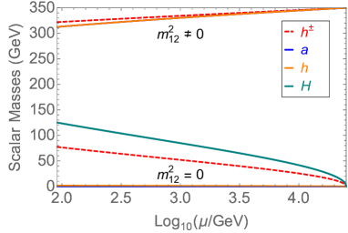
Figure 1: The Higgs mass spectrum in the MS-2HDM without and with soft breaking effects induced by $m^{2}_{12}$. For $m^{2}_{12}=0$, the CP-odd scalar $a$ remains massless at tree-level, whereas $h$ and $h^{\pm}$ receive small masses due to the $g^{\prime}$ and Yukawa coupling effects. For $m^{2}_{12}\neq 0$, one obtains a quasi-degenerate heavy Higgs spectrum, cf. (30). Here we have chosen $\mu_{X}=2.5\times 10^{4}$ GeV, $\lambda(\mu_{X})=0$ and $\tan\beta=50$ for illustration.

Therefore, $g^{\prime}$ and Yukawa coupling effects are not sufficient to yield a viable Higgs spectrum at the weak scale, starting from a SO(5)-invariant boundary condition at some high scale $\mu_{X}$. To minimally circumvent this problem, we include soft SO(5)-breaking effects, by assuming a non-zero soft-breaking term ${\rm Re}(m_{12}^{2})$. In the SO(5)-symmetric limit for the scalar quartic couplings, but with ${\rm Re}(m_{12}^{2})\neq 0$, we obtain the following mass spectrum [cf. (7a)-(7d)]:

$$M_{H}^{2}\ =\ 2\lambda_{2}v^{2}\;,\qquad M_{h}^{2}\ =\ M_{a}^{2}\ =\ M^{2}_{h^{\pm}}\ =\ \frac{{\rm Re}(m^{2}_{12})}{s_{\beta}c_{\beta}}\;,$$ (30)

as well as an equality between the CP-even and CP-odd mixing angles: $\alpha=\beta$, thus predicting an exact alignment for the SM-like Higgs boson $H$, simultaneously with an experimentally allowed heavy Higgs spectra (see Figure 1 for $m^{2}_{12}\neq 0$ case). Note that in the alignment limit, the heavy Higgs sector is exactly degenerate [cf. (30)] at the SO(5) symmetry-breaking scale, and at the low-energy scale, this degeneracy is mildly broken by the RG effects. Thus, we obtain a quasi-degenerate heavy Higgs spectrum, which is a unique prediction of the MS-2HDM, valid even in the non-decoupling limit, and can be used to distinguish this model from other 2HDM scenarios.

4.3 Misalignment Predictions

As discussed in Section 4.2, there will be some deviation from the alignment limit in the low-energy Higgs spectrum of the MS-2HDM due to RG and soft-breaking effects. By requiring that the mass and couplings of the SM-like Higgs boson $H$ are consistent with the latest Higgs data from the LHC [3], we derive predictions for the remaining scalar spectrum and compare them with the existing (in)direct limits on the heavy Higgs sector. For the SM-like Higgs boson mass, we use the $3\sigma$ allowed range from the recent CMS and ATLAS Higgs mass measurements [3, 40]: $M_{H}\in\big{[}124.1,~{}126.6\big{]}~{}{\rm GeV}$. For the Higgs couplings to the SM vector bosons and fermions, we use the constraints in the $(\tan\beta,~{}\beta-\alpha)$ plane derived from a recent global fit for the Type-II 2HDM [16]. For a given set of SO(5) boundary conditions $\big{\{}\mu_{X},\tan\beta(\mu_{X}),\lambda(\mu_{X})\big{\}}$, we thus require that the RG-evolved 2HDM parameters at the weak scale must satisfy the above constraints on the lightest CP-even Higgs boson sector. This requirement of alignment with the SM Higgs sector puts stringent constraints on the MS-2HDM parameter space, as shown in Figure 2 by the blue shaded region. In the red shaded region, there is no viable solution to the RG equations. We ensure that the remaining allowed (white) region satisfies the necessary theoretical constraints, i.e. positivity and vacuum stability of the Higgs potential, and perturbativity of the Higgs self-couplings [6]. From Figure 2, we find that there exists an upper limit of $\mu_{X}\lesssim 10^{9}$ GeV on the SO(5)-breaking scale of the 2HDM potential, beyond which an ultraviolet completion of the theory must be invoked. Moreover, for $10^{5}~{}{\rm GeV}\lesssim\mu_{X}\lesssim 10^{9}~{}{\rm GeV}$, only a narrow range of $\tan\beta$ values are allowed.

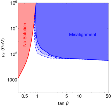
Figure 2: The $1\sigma$ (dotted), $2\sigma$ (dashed) and $3\sigma$ (solid) exclusion contours (blue shaded region) from the alignment constraints in MS-2HDM. The red shaded region is theoretically excluded, as there is no solution to the RG equations up to two-loop order in this region.

For the allowed parameter space of our MS-2HDM as shown in Figure 2, we obtain concrete predictions for the remaining Higgs spectrum. In particular, the alignment condition imposes a lower bound on the soft breaking parameter Re$(m^{2}_{12})$, and hence, on the heavy Higgs spectrum. The comparison of the existing global fit limit on the charged Higgs-boson mass as a function of $\tan\beta$ [16] with our predicted limits from the alignment condition in the MS-2HDM for a typical value of the boundary scale $\mu_{X}=3\times 10^{4}$ GeV is shown in Figure 3 (left panel). It is clear that the alignment limits are stronger than the global fit limits, except in the very small and very large $\tan\beta$ regimes. For $\tan\beta\lesssim 1$ region, the indirect limit obtained from the $Z\to b\bar{b}$ precision observable becomes the strictest [41, 16]. Similarly, for the large $\tan\beta\gtrsim 30$ case, the alignment limit can be easily obtained [cf. (20c)] without requiring a large soft-breaking parameter $m_{12}^{2}$, and therefore, the lower limit on the charged Higgs mass derived from the misalignment condition becomes somewhat weaker in this regime.

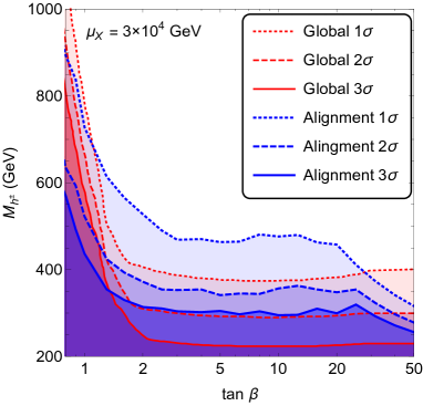
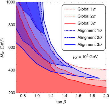
Figure 3: Left: The $1\sigma$ (dotted), $2\sigma$ (dashed) and $3\sigma$ (solid) lower limits on the charged Higgs mass obtained from the alignment condition (blue lines) in the MS-2HDM with $\mu_{X}=3\times 10^{4}$ GeV. Right: The $1\sigma$ (dotted), $2\sigma$ (dashed) and $3\sigma$ (solid) allowed regions from the alignment condition (blue lines) for $\mu_{X}=10^{5}$ GeV. For comparison, the corresponding lower limits from a global fit are also shown (red lines).

From Figure 2, it should be noted that for $\mu_{X}\gtrsim 10^{5}$ GeV, phenomenologically acceptable alignment is not possible in the MS-2HDM for large $\tan\beta$ and large $m^{2}_{12}$. Therefore, we also get an upper bound on the charged Higgs-boson mass $M_{h^{\pm}}$ from the misalignment condition, depending on $\tan\beta$. This is illustrated in Figure 3 (right panel) for $\mu_{X}=10^{5}$ GeV.

Similar alignment constraints are obtained for the heavy neutral pseudo-Goldstone bosons $h$ and $a$, which are predicted to be quasi-degenerate with the charged Higgs boson $h^{\pm}$ in the MS-2HDM [cf. (30)]. The current experimental lower limits on the heavy neutral Higgs sector [38] are much weaker than the alignment constraints in this case. Thus, the MS-2HDM scenario provides a natural reason for the absence of a heavy Higgs signal below the top-quark threshold, and this has important consequences for the heavy Higgs searches in the run-II phase of the LHC, as discussed in the following section.

5 Collider Signatures in the Alignment Limit

In the alignment limit, the couplings of the lightest CP-even Higgs boson are exactly similar to the SM Higgs couplings, while the heavy CP-even Higgs boson is gaugephobic [cf. (10)]. Therefore, two of the relevant Higgs production mechanisms at the LHC, namely, the vector boson fusion and Higgsstrahlung processes are suppressed for the heavy neutral Higgs sector. As a consequence, the only relevant production channels to probe the neutral Higgs sector of the MS-2HDM are the gluon-gluon fusion and $t\bar{t}h$ ($b\bar{b}h$) associated production mechanisms at low (high) $\tan\beta$. For the charged Higgs sector of the MS-2HDM, the dominant production mode is the associated production process: $gg\to\bar{t}bh^{+}+t\bar{b}h^{-}$, irrespective of $\tan\beta$.

Similarly, for the decay modes of the heavy neutral Higgs bosons in the MS-2HDM, the $t\bar{t}$ ($b\bar{b}$) channel is the dominant one for low (high) $\tan\beta$ values, whereas for the charged Higgs boson $h^{+(-)}$, the $t\bar{b}(\bar{t}b)$ mode is the dominant one for any $\tan\beta$. Thus, the heavy Higgs sector of the MS-2HDM can be effectively probed at the LHC through the final states involving third-generation quarks.

5.1 Charged Higgs Signal

The most promising channel at the LHC for the charged Higgs boson in the MS-2HDM is

$$gg\ \to\ \bar{t}bh^{+}+t\bar{b}h^{-}\ \to\ t\bar{t}b\bar{b}\;.$$ (31)

Experimentally, this is a challenging mode due to large QCD backgrounds and the non-trivial event topology, involving at least four $b$-jets [42]. Nevertheless, a recent CMS study [43] has presented for the first time a realistic analysis of this process, in the leptonic decay mode of the $W$’s coming from top decays:

$$gg\ \to\ h^{\pm}tb\ \to\ (\ell\nu_{\ell}bb)(\ell^{\prime}\nu_{\ell^{\prime}}b)b$$ (32)

($\ell,\ell^{\prime}$ beings electrons or muons). Using the $\sqrt{s}=8$ TeV LHC data, they have derived 95% CL upper limits on the production cross section $\sigma(gg\to h^{\pm}tb)$ times the branching ratio BR($h^{\pm}\to tb$) as a function of the charged Higgs mass, as shown in Figure 4. In the same Figure, we show the corresponding predictions at $\sqrt{s}=14$ TeV LHC in the Type-II MS-2HDM for some representative values of $\tan\beta$. The cross section predictions were obtained at leading order (LO) by implementing the 2HDM in MadGraph5_aMC@NLO [44] and using the NNPDF2.3 PDF sets [45]. A comparison of these cross sections with the CMS limit suggests that the run-II phase of the LHC might be able to probe the low $\tan\beta$ region of the MS-2HDM parameter space using the process (31). Note that the production cross section $\sigma(gg\to\bar{t}bh^{+})$ decreases rapidly with increasing $\tan\beta$ due to the Yukawa coupling suppression, even though BR($h^{+}\to\bar{t}b$) remains close to 100%. Therefore, this channel is only effective for low $\tan\beta$ values.

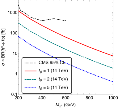
Figure 4: Predictions for the cross section of the process (31) in the Type-II MS-2HDM at $\sqrt{s}=14$ TeV LHC for various values of $\tan\beta$. For comparison, we have also shown the current 95% CL CMS upper limit from the $\sqrt{s}=8$ TeV data [43].

In order to make a rough estimate of the $\sqrt{s}=14$ TeV LHC sensitivity to the charged Higgs signal (31) in the MS-2HDM, we perform a parton level simulation of the signal and background events using MadGraph5 [44]. For the event reconstruction, we use some basic selection cuts on the transverse momentum, pseudo-rapidity and dilepton invariant mass, following the CMS analysis [43]:

$$p_{T}^{\ell}\ >\ 20~{}{\rm GeV},\quad|\eta^{\ell}|<2.5,\quad p_{T}^{j}\ >\ 30~{}{\rm GeV},\quad|\eta^{j}|<2.4,\quad\not{E}_{T}>40~{}{\rm GeV}$$

$$\Delta R^{\ell\ell}>0.4,\quad\Delta R^{\ell j}>0.4,\quad M_{\ell\ell}>12~{}{\rm GeV},\quad|M_{\ell\ell}-M_{Z}|>10~{}{\rm GeV}.$$ (33)

Jets are reconstructed using the anti-$k_{T}$ clustering algorithm [46] with a distance parameter of 0.5. Since four $b$-jets are expected in the final state, at least two $b$-tagged jets are required in the signal events, and we assume the $b$-tagging efficiency for each of them to be 70%.

The inclusive SM cross section for $pp\to t\bar{t}b\bar{b}+X$ is $\sim 18$ pb at NLO, with roughly 30% uncertainty due to higher order QCD corrections [47]. Most of the QCD background for the $4b+2\ell+\not{E}_{T}$ final state given by (32) can be reduced significantly by reconstructing at least one top-quark. The remaining irreducible background due to SM $t\bar{t}b\bar{b}$ production can be suppressed with respect to the signal by reconstructing the charged Higgs boson mass, once a valid signal region is defined, e.g. in terms of an observed excess of events at the LHC in future. For the semi-leptonic decay mode of top-quarks as in (32), one cannot directly use an invariant mass observable to infer $M_{h^{\pm}}$, as both the neutrinos in the final state give rise to missing momentum. A useful quantity in this case is the $M_{T2}$ variable [48], defined as

$$M_{T2}\ =\ \underset{\left\{\not{\mathbf{p}}_{T_{\rm a}}+\not{\mathbf{p}}_{T_{\rm b}}=\not{\mathbf{p}}_{T}\right\}}{\rm min}\Big{[}{\rm max}\left\{m_{T_{\rm a}},m_{T_{\rm b}}\right\}\Big{]}\;,$$ (34)

where $\{{\rm a}\},\{\rm b\}$ stand for the two sets of particles in the final state, each containing a neutrino with part of the missing transverse momentum ($\not{\mathbf{p}}_{T_{\rm{a,b}}}$). Minimization over all possible sums of these two momenta gives the observed missing transverse momentum $\not{\mathbf{p}}_{T}$, whose magnitude is the same as $\not{E}_{T}$ in our specific case. In (34), $m_{T_{i}}$ (with $i=$a,b) is the usual transverse mass variable for the system $\{i\}$, defined as

$$m_{T_{i}}^{2}\ =\ \left(\sum_{\rm visible}E_{T_{i}}+\not{E}_{T_{i}}\right)^{2}-\left(\sum_{\rm visible}{\mathbf{p}}_{T_{i}}+\not{\mathbf{p}}_{T_{i}}\right)^{2}\;.$$ (35)

For the correct combination of the final state particles in (32), i.e. for $\{{\rm a}\}=(\ell\nu_{\ell}bb)$ and $\{{\rm b}\}=(\ell^{\prime}\nu_{\ell^{\prime}}bb)$ in (34), the maximum value of $M_{T2}$ represents the charged Higgs boson mass, with the $M_{T2}$ distribution smoothly dropping to zero at this point. This is illustrated in Figure 5 for a typical choice of $M_{h^{\pm}}=300$ GeV. For comparison, we also show the $M_{T2}$ distribution for the SM background, which obviously does not have a sharp endpoint. Thus, for a given hypothesized signal region defined in terms of an excess due to $M_{h^{\pm}}$, we may impose an additional cut on $M_{T2}\leq M_{h^{\pm}}$ to enhance the signal (32) over the irreducible SM background.

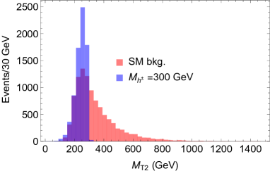
Figure 5: An illustration of the charged Higgs boson mass reconstruction using the $M_{T2}$ variable. The irreducible SM background distribution is also shown for comparison.

Assuming that the charged Higgs boson mass can be reconstructed efficiently, we present an estimate of the signal to background ratio for the charged Higgs signal given by (31) at $\sqrt{s}=14$ TeV LHC with 300 fb^-1 for some typical values of $\tan\beta$ in Figure 6. Since the mass of the charged Higgs boson is a priori unknown, we vary the charged Higgs mass, and for each value of $M_{h^{\pm}}$, we assume that it can be reconstructed around its actual value within 30 GeV uncertainty.

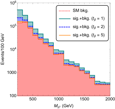
Figure 6: Predicted number of events for the dominant charged Higgs signal in the MS-2HDM at $\sqrt{s}=14$ TeV LHC with $300~{}{\rm fb}^{-1}$ integrated luminosity. The irreducible SM background (red shaded) is controlled by assuming an efficient mass reconstruction technique [23].

5.2 Heavy Neutral Higgs Signal

So far there have been no direct searches for heavy neutral Higgs bosons involving $t\bar{t}$ and/or $b\bar{b}$ final states, mainly due to the challenges associated with uncertainties in the jet energy scales and the combinatorics arising from complicated multiparticle final states in a busy QCD environment. Nevertheless, these channels become pronounced in the MS-2HDM scenario, and hence, we have made a preliminary attempt to study them in [23]. In particular, we focus on the search channel

$$gg\ \to\ t\bar{t}h\ \to\ t\bar{t}t\bar{t}\;.$$ (36)

Such four top final states have been proposed before in the context of other exotic searches at the LHC (see e.g. [49]). However, their relevance for heavy Higgs searches have not been explored so far. We note here that the existing 95% CL experimental upper limit on the four top production cross section is 59 fb from ATLAS [50] and 32 fb from CMS [51], whereas the SM prediction for the inclusive cross section of the process $pp\to t\bar{t}t\bar{t}+X$ is about 10-15 fb [52].

To get a rough estimate of the signal to background ratio for our four-top signal (36), we perform a parton-level simulation of the signal and background events at LO in QCD using MadGraph5_aMC@NLO [44] with NNPDF2.3 PDF sets [45]. For the inclusive SM cross section for the four-top final state at $\sqrt{s}=14$ TeV LHC, we obtain 11.85 fb, whereas our proposed four-top signal cross sections are found to be comparable or smaller depending on $M_{h}$ and $\tan\beta$, as shown in Figure 7. However, since we expect one of the $t\bar{t}$ pairs coming from an on-shell $h$ decay to have an invariant mass around $M_{h}$, we can use this information to significantly boost the signal over the irreducible SM background. Note that all the predicted cross sections shown in Figure 7 are well below the current experimental upper bound [51].

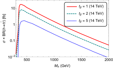
Figure 7: Predictions for the cross section of the process (36) in the Type-II MS-2HDM at $\sqrt{s}=14$ TeV LHC for various values of $\tan\beta$.

Depending on the $W$ decay mode from $t\to Wb$, there are 35 final states for four top decays. According to a recent ATLAS analysis [53], the experimentally favored channel is the semi-leptonic/hadronic final state with two same-sign isolated leptons. Although the branching fraction for this topology (4.19%) is smaller than most of the other channels, the presence of two same-sign leptons in the final state allows us to reduce the large QCD background substantially, including that due to the SM production of $t\bar{t}b\bar{b}+$jets [53]. Therefore, we will only consider the following decay chain in our preliminary analysis:

$$gg\ \to\ t\bar{t}h\ \to\ (t\bar{t})(t\bar{t})\ \to\ \Big{(}(\ell^{\pm}\nu_{\ell}b)(jjb)\Big{)}\Big{(}(\ell^{\prime\pm}\nu_{\ell^{\prime}}b)(jjb)\Big{)}\;.$$ (37)

For event reconstruction, we will use the same selection cuts as in (33), and in addition, following [53], we require the scalar sum of the $p_{T}$ of all leptons and jets (defined as $H_{T}$) to exceed 350 GeV.

As in the charged Higgs boson case (cf. Figure 5), the heavy Higgs mass can be reconstructed from the signal given by (37) using the $M_{T2}$ endpoint technique, and therefore, an additional selection cut on $M_{T2}\leq M_{h}$ can be used to enhance the signal over the irreducible background. Our simulation results for the predicted number of signal and background events for the process (37) at $\sqrt{s}=14$ TeV LHC with 300 fb^-1 luminosity are shown in Figure 8. The signal events are shown for three representative values of $\tan\beta$. Here we vary the a priori unknown heavy Higgs mass, and for each value of $M_{h}$, we assume that it can be reconstructed around its actual value within 30 GeV uncertainty. From this preliminary analysis, we find that the $t\bar{t}t\bar{t}$ channel provides the most promising collider signal to probe the heavy Higgs sector in the MS-2HDM at low values of $\tan\beta\lesssim 5$.

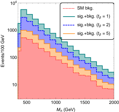
Figure 8: Predicted number of events for the $t\bar{t}t\bar{t}$ signal from the neutral pseudo-Goldstone boson in the MS-2HDM at $\sqrt{s}=14$ TeV LHC with $300~{}{\rm fb}^{-1}$ integrated luminosity.

The above analysis is also applicable for the CP-odd Higgs boson $a$, which has similar production cross sections and $t\bar{t}$ branching fractions as the CP-even Higgs $h$. However, the $t\bar{t}h(a)$ production cross section as well as the $h(a)\to t\bar{t}$ branching ratio decreases with increasing $\tan\beta$. This is due to the fact that the $ht\bar{t}$ coupling in the alignment limit is $\cos\alpha/\sin\beta\sim\cot\beta$, which is same as the $at\bar{t}$ coupling. Thus, the high $\tan\beta$ region of the MS-2HDM cannot be searched via the $t\bar{t}t\bar{t}$ channel proposed above, and one needs to consider the channels involving down-sector Yukawa couplings, e.g. $b\bar{b}b\bar{b}$ and $b\bar{b}\tau^{+}\tau^{-}$ [42]. It is also worth commenting here that the simpler process $pp\to h/a\to t\bar{t}~{}(b\bar{b})$ at low (high) $\tan\beta$ suffers from a huge SM $t\bar{t}$ ($b\bar{b}$) QCD background, even after imposing an $M_{t\bar{t}~{}(b\bar{b})}$ cut. Some parton-level studies of this signal in the context of MSSM have been performed in [54].

We should clarify that the results obtained in this section are valid only at the parton level. In a realistic detector environment, the sharp features of the signal [see e.g., Figure 5] used to derive the sensitivity reach in Figures 6 and 8 may not survive, and therefore, the signal-to-background ratio might get somewhat reduced than that shown here. A detailed detector-level analysis of these signals, including realistic top reconstruction efficiencies and smearing effects, is currently being pursued in a separate dedicated study.

6 Conclusions

We provide a symmetry justification of the so-called SM alignment limit, independently of the heavy Higgs spectrum and the value of $\tan\beta$ in the 2HDM. We show that in the 2HDMs where both Higgs doublets acquire VEVs, there exist only three different symmetry realizations, which could lead to the SM alignment by satisfying the natural alignment condition (22) for any value of $\tan\beta$. In the context of the Maximally Symmetric 2HDM based on the SO(5) group, we demonstrate how small deviations from this alignment limit are naturally induced by RG effects due to the hypercharge gauge coupling $g^{\prime}$ and third generation Yukawa couplings, which explicitly break the custodial symmetry of the theory. In addition, a non-zero soft SO(5)-breaking mass parameter is required to yield a viable Higgs spectrum consistent with the existing experimental constraints. Using the current Higgs signal strength data from the LHC, which disfavor large deviations from the alignment limit, we derive important constraints on the 2HDM parameter space. In particular, we predict lower limits on the mass scale of the heavy Higgs spectrum, which prevail the present global fit limits in a wide range of parameter space. Depending on the energy scale where the maximal symmetry could be realized in nature, we also obtain an upper limit on the heavy Higgs masses in certain cases, which could be probed during the run-II phase of the LHC. In addition, we have studied the collider signatures of the heavy Higgs sector in the alignment limit beyond the top-quark threshold. We find that the final states involving third-generation quarks can become a valuable observational tool to directly probe the heavy Higgs sector of the 2HDM in the alignment limit for low values of $\tan\beta$. Finally, we emphasize the importance of both charged and neutral heavy Higgs searches in order to unravel the doublet nature of the heavy Higgs sector.

References

References

- [1] G. Aad et al. [ATLAS Collaboration], Phys. Lett. B 716, 1 (2012); S. Chatrchyan et al. [CMS Collaboration], Phys. Lett. B 716, 30 (2012).
- [2] P. W. Higgs, Phys. Rev. Lett. 13, 508 (1964); F. Englert and R. Brout, Phys. Rev. Lett. 13, 321 (1964); G. S. Guralnik, C. R. Hagen and T. W. B. Kibble, Phys. Rev. Lett. 13, 585 (1964).
- [3] ATLAS collaboration, ATLAS-CONF-2014-009; V. Khachatryan et al. [CMS Collaboration], arXiv:1412.8662 [hep-ex].
- [4] H. E. Haber and G. L. Kane, Phys. Rept. 117, 75 (1985).
- [5] J. E. Kim, Phys. Rept. 150, 1 (1987).
- [6] G. C. Branco, P. M. Ferreira, L. Lavoura, M. N. Rebelo, M. Sher and J. P. Silva, Phys. Rept. 516, 1 (2012).
- [7] T. D. Lee, Phys. Rev. D 8, 1226 (1973); Phys. Rept. 9, 143 (1974).
- [8] H. Georgi, Hadronic J. 1, 155 (1978); Y. L. Wu and L. Wolfenstein, Phys. Rev. Lett. 73, 1762 (1994).
- [9] V. Silveira and A. Zee, Phys. Lett. B 161, 136 (1985).
- [10] V. A. Kuzmin, V. A. Rubakov and M. E. Shaposhnikov, Phys. Lett. B 155, 36 (1985).
- [11] R. A. Battye, G. D. Brawn and A. Pilaftsis, JHEP 1108, 020 (2011).
- [12] S. L. Glashow and S. Weinberg, Phys. Rev. D 15, 1958 (1977); E. A. Paschos, Phys. Rev. D 15, 1966 (1977).
- [13] H. E. Haber, G. L. Kane and T. Sterling, Nucl. Phys. B 161, 493 (1979).
- [14] ATLAS collaboration, ATLAS-CONF-2014-010; V. Khachatryan et al. [CMS Collaboration], Phys. Rev. D 90, 112013 (2014).
- [15] A. Celis, V. Ilisie and A. Pich, JHEP 1307, 053 (2013); C. W. Chiang and K. Yagyu, JHEP 1307, 160 (2013); C.-Y. Chen, S. Dawson and M. Sher, Phys. Rev. D 88, 015018 (2013); N. Craig, J. Galloway and S. Thomas, arXiv:1305.2424 [hep-ph]; K. Cheung, J. S. Lee and P.-Y. Tseng, JHEP 1401, 085 (2014); L. Wang and X.-F. Han, JHEP 1411, 085 (2014); B. Dumont, J. F. Gunion, Y. Jiang and S. Kraml, Phys. Rev. D 90, 035021 (2014); S. Kanemura, K. Tsumura, K. Yagyu and H. Yokoya, Phys. Rev. D 90, 075001 (2014); D. Chowdhury and O. Eberhardt, arXiv:1503.08216 [hep-ph].
- [16] O. Eberhardt, U. Nierste and M. Wiebusch, JHEP 1307, 118 (2013); J. Baglio, O. Eberhardt, U. Nierste and M. Wiebusch, Phys. Rev. D 90, 015008 (2014).
- [17] P. H. Chankowski, T. Farris, B. Grzadkowski, J. F. Gunion, J. Kalinowski and M. Krawczyk, Phys. Lett. B 496, 195 (2000).
- [18] J. F. Gunion and H. E. Haber, Phys. Rev. D 67, 075019 (2003).
- [19] I. F. Ginzburg and M. Krawczyk, Phys. Rev. D 72, 115013 (2005).
- [20] A. Delgado, G. Nardini and M. Quiros, JHEP 1307, 054 (2013).
- [21] M. Carena, I. Low, N. R. Shah and C. E. M. Wagner, JHEP 1404, 015 (2014).
- [22] G. Bhattacharyya and D. Das, Phys. Rev. D 91, 015005 (2015).
- [23] P. S. B. Dev and A. Pilaftsis, JHEP 1412, 024 (2014).
- [24] H. E. Haber and R. Hempfling, Phys. Rev. D 48, 4280 (1993).
- [25] A. Pilaftsis and C. E. M. Wagner, Nucl. Phys. B 553, 3 (1999).
- [26] M. Carena, H. E. Haber, I. Low, N. R. Shah and C. E. M. Wagner, Phys. Rev. D 91, 035003 (2015).
- [27] P. M. Ferreira, H. E. Haber and J. P. Silva, Phys. Rev. D 79, 116004 (2009); P. M. Ferreira, H. E. Haber, M. Maniatis, O. Nachtmann and J. P. Silva, Int. J. Mod. Phys. A 26, 769 (2011).
- [28] M. Maniatis, A. von Manteuffel, O. Nachtmann and F. Nagel, Eur. Phys. J. C 48, 805 (2006).
- [29] C. C. Nishi, Phys. Rev. D 83, 095005 (2011).
- [30] A. Pilaftsis, Phys. Lett. B 706, 465 (2012).
- [31] M. Maniatis, A. von Manteuffel and O. Nachtmann, Eur. Phys. J. C 57, 719 (2008); I. P. Ivanov, Phys. Rev. D 77, 015017 (2008); C. C. Nishi, Phys. Rev. D 77, 055009 (2008).
- [32] J. F. Gunion and H. E. Haber, Phys. Rev. D 72, 095002 (2005); M. Maniatis and O. Nachtmann, JHEP 1111, 151 (2011).
- [33] N. G. Deshpande and E. Ma, Phys. Rev. D 18, 2574 (1978).
- [34] R. Barbieri, L. J. Hall and V. S. Rychkov, Phys. Rev. D 74, 015007 (2006).
- [35] R. Slansky, Phys. Rept. 79, 1 (1981); H. Georgi, Lie Algebras in Particle Physics, Westview Press (1999).
- [36] B. C. Hall, Lie Groups, Lie Algebras, and Representations, Springer-Verlag (2003).
- [37] J. Goldstone, Nuovo Cim. 19, 154 (1961).
- [38] K. A. Olive et al. (Particle Data Group), Chin. Phys. C 38, 090001 (2014) [http://pdg.lbl.gov/].
- [39] R. D. Peccei and H. R. Quinn, Phys. Rev. Lett. 38, 1440 (1977).
- [40] G. Aad et al. [ATLAS Collaboration], Phys. Rev. D 90, 052004 (2014).
- [41] O. Deschamps, S. Descotes-Genon, S. Monteil, V. Niess, S. T’Jampens and V. Tisserand, Phys. Rev. D 82, 073012 (2010).
- [42] S. Heinemeyer et al. [LHC Higgs Cross Section Working Group Collaboration], arXiv:1307.1347 [hep-ph].
- [43] CMS Collaboration, CMS-PAS-HIG-13-026.
- [44] J. Alwall et al., JHEP 1407, 079 (2014); https://launchpad.net/mg5amcnlo.
- [45] R. D. Ball et al., Nucl. Phys. B 867, 244 (2013); https://nnpdf.hepforge.org/
- [46] M. Cacciari, G. P. Salam and G. Soyez, JHEP 0804, 063 (2008).
- [47] G. Bevilacqua, M. Czakon, C. G. Papadopoulos, R. Pittau and M. Worek, JHEP 0909, 109 (2009).
- [48] C. G. Lester and D. J. Summers, Phys. Lett. B 463, 99 (1999).
- [49] M. Spira and J. D. Wells, Nucl. Phys. B 523, 3 (1998); A. Pomarol and J. Serra, Phys. Rev. D 78, 074026 (2008); K. Kumar, T. M. P. Tait and R. Vega-Morales, JHEP 0905, 022 (2009); S. Jung and J. D. Wells, JHEP 1011, 001 (2010); G. L. Kane, E. Kuflik, R. Lu and L. T. Wang, Phys. Rev. D 84, 095004 (2011); G. Cacciapaglia, R. Chierici, A. Deandrea, L. Panizzi, S. Perries and S. Tosi, JHEP 1110, 042 (2011).
- [50] ATLAS Collaboration, ATLAS-CONF-2013-051.
- [51] V. Khachatryan et al. [CMS Collaboration], JHEP 1411, 154 (2014); J. Keaveney, arXiv:1412.4641 [hep-ex].
- [52] G. Bevilacqua and M. Worek, JHEP 1207, 111 (2012).
- [53] D. Paredes [ATLAS Collaboration], PhD Thesis, Université Blaise Pascal (2013), CERN-THESIS-2013-202.
- [54] S. Moretti and D. A. Ross, Phys. Lett. B 712, 245 (2012); A. Djouadi and J. Quevillon, JHEP 1310, 028 (2013); A. Djouadi, L. Maiani, A. Polosa, J. Quevillon and V. Riquer, arXiv:1502.05653 [hep-ph].