Formalising Hypothesis Virtues in Knowledge Graphs: A General Theoretical Framework and its Validation in Literature-Based Discovery Experiments

Abstract

We introduce an approach to discovery informatics that uses so called knowledge graphs as the essential representation structure. Knowledge graph is an umbrella term that subsumes various approaches to tractable representation of large volumes of loosely structured knowledge in a graph form. It has been used primarily in the Web and Linked Open Data contexts, but is applicable to any other area dealing with knowledge representation. In the perspective of our approach motivated by the challenges of discovery informatics, knowledge graphs correspond to hypotheses. We present a framework for formalising so called hypothesis virtues within knowledge graphs. The framework is based on a classic work in philosophy of science, and naturally progresses from mostly informative foundational notions to actionable specifications of measures corresponding to particular virtues. These measures can consequently be used to determine refined sub-sets of knowledge graphs that have large relative potential for making discoveries. We validate the proposed framework by experiments in literature-based discovery. The experiments have demonstrated the utility of our work and its superiority w.r.t. related approaches.

1 Introduction

Ever since the dawn of computer age, researchers have been intrigued by the possibility of automating the process of discovery [27]. Today, the field of discovery informatics is getting more relevant than ever before. The large amounts of data that are being made openly available for anyone to explore have an immense potential for making new discoveries, and solutions that would enable this are highly sought after [15].

Knowledge graphs are one of the most universal ways of representing actionable, data-driven knowledge at large scale [8]. They represent knowledge as relationships (edges) between items of interests (vertices), with the possibility of adding additional annotations representing for instance multiple relationship types (i.e., predicates). Such a representation has many advantages like universal applicability and a wealth of well-founded methods for analysing graph structures. Yet the full potential of knowledge graphs for practical applications in knowledge discovery is still largely to be explored [8].

The motivation of the presented work is two-fold. Firstly, we want to propose a general framework for defining features of knowledge graphs that can determine which parts of the graphs have highest potential for making discoveries. We believe that this can facilitate the process of semi-automated knowledge discovery in domains that have a lot of data available in graph-like format, but suffer from high redundancy and noise (e.g., World Wide Web, social networks or biological pathway databases).

The second motivation is more practical. In our previous work [30], we addressed the problem of extracting simple knowledge graphs from biomedical texts. The graphs were then used for so called machine-aided skim reading – high-level navigation of a specific domain represented by a textual corpus which was assumed to facilitate the discovery process. Indeed, even highly experienced domain experts were able to discover new and relevant facts using the prototype system. However, the results also contained some noise and connections that were correct, but rather obvious and/or uninteresting. This motivated the validation experiments presented here, which demonstrate that our framework for formalising hypothesis virtues can tackle the problems of noise, redundancy and obviousness in knowledge graphs automatically extracted from texts.

Our approach consists of formalising features applicable to ranking knowledge graphs (or their partitions) based on their potential for making discoveries. This can be used for instance for decomposing knowledge graphs into atomic subgraphs and consequent construction of a graph that has higher “discovery potential” than the original one. The formalisation is based on widely accepted hypothesis virtues studied in philosophy of science [36]. Examples of virtues are refutability or generality – a good scientific hypothesis has to be falsifiable and should also provide explanations of phenomena outside of its original scope. We present general conditions for each of the virtues and proceed with defining specific measures that conform to these conditions and can be efficiently implemented.

The validation of the approach was performed in the context of literature-based discovery [41]. We extracted knowledge graphs from two de facto standard biomedical corpora traditionally used in evaluation of literature-based discovery tools. For that we used a very simple and domain-agnostic method that extracts statistically significant co-occurrence relationships. We opted for such a solution to demonstrate the universal applicability of our approach. From these basic graphs, we constructed refined ones using a genetic algorithm that utilises the hypothesis virtue measures in the fitness function. The refined graphs were analysed according to the evaluation measures used in the literature-based discovery field and compared to related works. The results of the validation were positive, as we outperformed the state of the art in most respects. Moreover, we discovered relevant relationships that have not been covered by any related automated system or manual study. This demonstrates the practical utility of our approach.

Our main contributions are as follows. We have proposed a novel theoretical framework for extensible definition of measures that can be used to analyse the discovery potential of knowledge graphs. We have defined specific measures applicable especially to refinement of knowledge graphs automatically extracted from texts. We have implemented an evolutionary method for refinement of the automatically extracted knowledge graphs that is applicable out-of-the-box to any domain where English texts are available. We have demonstrated the practical relevance of the presented research by a successful experimental validation in the field of literature-based discovery. Last but not least, we have provided a data package containing a prototype implementation of our approach, results and other data necessary for the replication of our experiments.

The rest of the article is organised as follows. Section 2 presents the general framework for formalising the hypothesis virtues in the context of knowledge graphs. Section 3 then introduces actual measures that follow the general requirements of the hypothesis virtue formalisations. Our approach is experimentally validated in Section 4. The section describes the evolutionary refinement of knowledge graphs extracted from texts and elaborates on the experiments in literature-based discovery. Related approaches are discussed in Section 5. Finally, we conclude the article and outline our future work in Section 6.

2 Formalising Hypothesis Virtues

The foundations of the presented work are built on [36], a classic work in philosophy of science. The work introduces five virtues of hypothesis: conservatism, modesty, simplicity, generality and refutability. These virtues present a comprehensive compilation of the philosophical treatments of discovery ranging from antiquity to modern analytical philosophy, and have been frequently used as a reference for determining quality of hypotheses in science.

According to [36], the virtue of conservatism reflects the fact that good hypothesis usually makes rather conservative claims. This is to minimise the risk of error by reaching too far from the state of the art in one step (even though the combination of the particular conservative claims may go very far after all, indeed). Modesty is related to conservatism – a hypothesis A is more modest than A and B (since A and B entails A), and a more modest hypothesis is considered better as it minimises the risk of wrong and/or redundant claims. The simplicity virtue posits that a good hypothesis should simplify our view of the world by making new claims about it, even though the claims themselves may actually be quite complex. The generality virtue is related to the predictive power of hypothesis – the more phenomena (that have perhaps not even been considered originally) it can explain, the better it is. Finally, refutability means that a hypothesis should be falsifiable in as obvious manner as possible. This is a factor of utmost importance, as discussed in arguably the most influential work on this topic [33].

In the following, we first define the notions of hypotheses and their claims in the context of knowledge graphs (Section 2.1) and then continue with formalising the five virtues (Section 2.2).

2.1 Preliminaries

First we define a universe – a general knowledge graph within which particular hypotheses may be defined.

Definition 1

A universe graph $U$ is a tuple $(V_{U},E_{U},\Lambda_{V},\Lambda_{E})$ where $V_{U}$ is a set of vertices, $E_{U}\subseteq V_{U}\times V_{U}$ is a set of edges and $\Lambda_{V},\Lambda_{E}$ are sets of labeling maps (i.e., morphisms) that associate values with the universe vertices and edges, respectively.

The labeling maps can, for instance, assign predicate types to edges in semantic networks, assert vertex types like class or individual in ontology knowledge graphs, or associate confidence weights with edges of automatically extracted knowledge graphs. Such a definition can accommodate a broad range of knowledge graphs with varying levels of semantic complexity, while keeping the basic structure still compatible with the analysis methods introduced here. The universe can be either directed or undirected. The experiments presented in this article deal with an undirected universe and therefore we assume undirected graphs in the following unless explicitly stated otherwise.

A hypothesis in a universe is defined as follows.

Definition 2

A hypothesis $H=(V_{H},E_{H},\Lambda_{V}^{H},\Lambda_{E}^{H})$ is a subgraph of the universe $U$ such that $V_{H}\subseteq V_{U},E_{H}\subseteq E_{U}$ and $\forall\lambda_{V}^{H}\in\Lambda_{V}^{H}\;\exists\lambda_{V}\in\Lambda_{V}.\;\lambda_{V}^{H}\subseteq\lambda_{V},\;\forall\lambda_{E}^{H}\in\Lambda_{E}^{H}\;\exists\lambda_{E}\in\Lambda_{E}.\;\lambda_{E}^{H}\subseteq\lambda_{E}$.

The second defining condition of the hypothesis subgraph means that any specific labeling map employed by a hypothesis has to be subsumed by a map defined in the universe. This ensures that the universe is closed w.r.t. possible interpretations of the hypotheses existing within it.

Most of the hypothesis virtues critically depend on what a claim of a hypothesis is, and therefore we need to define that as well.

Definition 3

A claim of a hypothesis $H$ is a simple (i.e., acyclic) path in the graph $H$.

Such a definition presents arguably the most universal view on what a particular knowledge graph may express. No matter what the actual semantics of the relationships in a hypothesis graph are, one can always study what they claim at least in terms of connections of vertices by means of edges, i.e., paths (we will use the terms path and claim interchangeably in the rest of the article). This makes our approach applicable to any type of knowledge graph.

Note that one practical implication of the last definition is that we can consider only connected graphs as hypotheses – if there is no path between two vertices, no claim is being made about them and they should thus be parts of different hypotheses. This is partly related to the open/closed world assumption dichotomy. The fact there is no connection between vertices does not mean no such connection can exist, it only means nothing is known about it in the context of the given knowledge graph.

The final preliminary definition concerns all claims possibly made by a hypothesis.

Definition 4

A claim set of a hypothesis $H$ is the set $\Pi(H)$ of all simple paths in the corresponding graph. A claim volume of $H$ is the size of its claim set, i.e., $|\Pi(H)|$.

The claim volume can be very large and is hard to compute even for relatively small graphs [47]. Also, it is not realistic to expect every possible path in a knowledge graph to convey a meaningful claim. Therefore in practice, it is convenient to restrict the claim set to a more manageable size based on case-specific heuristics. However, the maximal possible number of claims is apt as a theoretical notion for describing general knowledge graphs without further information about their domain and more complex semantics.

2.2 Formalising the Virtues

The following five sections present formalisations of the particular hypothesis virtues using the preliminary notions introduced above. Note that we provide general guidelines for measuring the virtues first, giving minimalistic set of conditions the measures should satisfy. Detailed examples of specific measures facilitating literature-based discovery are discussed in Sections 3 and 4.

2.2.1 Conservatism

Conservative claims should make small steps in a particular direction, however, the combination of the steps can potentially be quite radical (i.e., far-reaching). The conservatism of a path in a hypothesis $H$ can be measured by a function $f:\Pi(H)\rightarrow\mathbb{R}$ that satisfies the following conditions:

1. Assuming a metric $\delta:V_{U}\times V_{U}\rightarrow\mathbb{R}$ on the vertices in the universe graph, the function $f$ applied to a path $p=(v_{1},v_{2},\dots,v_{|p|})$ is negatively correlated with the $g(\{\delta(v_{1},v_{2}),\delta(v_{2},v_{3}),\dots,\delta(v_{|p|-1},v_{|p|})\})$ value, where $g:2^{\mathbb{R}}\rightarrow\mathbb{R}$ is an aggregation function (e.g., sum, mimimum, maximum or arithmetic mean).

2. If radical claims are preferred, then there is an additional requirement for $f$ being positively correlated with the $\delta(v_{1},v_{|p|})$ value.

The conservatism of the whole hypothesis $H$ is computed by aggregating all path conservatism measures across the $\Pi(H)$ set. The higher the aggregate value, the larger the conservatism. Due to the complexity of enumerating the $\Pi(H)$ set, practical conservatism measures can target only a subset of all possible paths. For instance, a set of shortest paths between all vertices in $H$ w.r.t. the $\delta$ edge labeling is a viable option as it is comparatively easier to compute and already satisfies condition 1. if sum is used as an aggregation function.

2.2.2 Modesty

Let us refer by $H_{\omega}$ to the complete graph corresponding to a hypothesis $H$ (i.e., a graph with an edge between any two vertices in $V_{H}$). Then the modesty of $H$ can be defined as

$$\frac{|\Pi(H_{\omega})|}{|\Pi(H)|}.$$

This number reflects the ratio between all possible claims about the entities covered by $H$ and the actual number of claims being made. The higher the ratio, the larger the modesty (a modest hypothesis minimises the number of claims made in relation to the number of claims that can possibly be made).

As mentioned before, computing the number of all simple paths in a graph is extremely difficult in general. Therefore in practice, approximations of the modesty measure are necessary. The approximations, however, should be monotonic w.r.t. the ideal modesty measure: assuming $f,g$ as the ideal and approximate modesty measures, respectively, then $g(H)>g(I)$ if and only if $f(H)>f(I)$ for any two hypotheses $H,I$.

2.2.3 Simplicity

For this virtue, we use the dual notion of complexity which has been extensively studied in the context of graphs [25]. A good hypothesis should simplify our view of the world despite of possibly being locally complex [36]. In order to formalise this intuition, let us assume the simplicity of a graph is measured by a function $f:\mathcal{G_{U}}\rightarrow\mathbb{R}$, where $\mathcal{G_{U}}$ is a set of all graphs conceivable in the universe $U$. The function $f$ should satisfy these conditions:

1. Given a hypothesis graph $H$ and a graph complexity measure $c:\mathcal{G_{U}}\rightarrow\mathbb{R}$, $f$ is positively correlated with the expression

   $$\frac{c(U\setminus H)}{c(U)}$$

   which reflects the universe simplification rate w.r.t. to the hypothesis.

2. If locally complex hypotheses are preferred, then the function $f$ is also required to be positively correlated with the value $c(H)$.

Strictly speaking, the rate in the first condition should also be higher than $1$ in order for the hypothesis to make the universe actually simpler, but practical applications may relax that requirement and just rank the hypotheses based on the measure.

2.2.4 Generality

Generality can be quantified as a number of explanations (i.e., claims) the hypothesis $H$ can provide for ‘out-of-scope’ phenomena (i.e., vertices) in the $U\setminus H$ graph. This can be expressed as

$$g(\{f(u)|u\in V_{U}\setminus V_{H}\}),$$

where the function $g:2^{\mathbb{R}}\rightarrow\mathbb{R}$ is an aggregation (like sum or arithmetic mean) over all vertices that are out of the $H$ scope. The function $f:V_{U}\rightarrow\mathbb{R}$ is required to be positively correlated with the $h(\{|\{v|v\in p\wedge v\in V_{H}\}|\;|\;p\in\Pi_{u}(U)\})$ value, where $h:2^{\mathbb{R}}\rightarrow\mathbb{R}$ is another aggregation function and $\Pi_{u}(U)$ is a set of all simple paths in the universe $U$ that start in the vertex $u$.

The generality definition reflects the basic intuition that the higher the number of $H$ vertices on paths explaining phenomena outside of $H$, the higher the generality of $H$. As the numbers of simple paths can be difficult to compute even if limited to paths starting in single nodes, approximations of this measure are needed for implementations again. Similarly to the modesty condition, we require the approximations to be monotonic w.r.t. the ideal generality measure.

2.2.5 Refutability

Refutability can be seen as a quantification of: 1) the easiness with which the claim volume $|\Pi(H)|$ of a particular hypothesis graph $H$ can be reduced; 2) the rate of the reduction. The atomic part of the process of refutation in the context of knowledge graphs is an invalidation, i.e., removal, of a vertex. Let us assume a decreasing ranking $R:\mathbb{N}\rightarrow V_{U}$ of the vertices in $H$ based on the number of simple paths that no longer exist in the graph after the vertex removal. Then we can define a top-k refutability as

$$\frac{|\Pi(H)|}{|\Pi(H)|+\sum_{i=1}^{k}|\Pi(H/R(i))|},$$

where $H/R(i)$ is a graph resulting from removal of the first vertex in the ranking $R$ from the graph $H/R(i-1)$. We assert $H/R(0)=H$ by definition. The lower the number of paths still existing after removing the top vertex according to $R$, the higher the refutability. The $|\Pi(H)|$ expression is added to the denominator to avoid potential division by zero, and also to normalise the measure value.

Note that for growing $k$ values, the top-k refutability generally converges to similar values for any given set of hypotheses as the measure is relative to the total number of paths in the graph. Therefore it is practical to use the measure with rather low $k$ values, perhaps even as low as $1$ which measures the rate of refutability in a single vertex removal step. Additionally, the ideal measure is difficult to compute and approximations are required in practice again. In particular, one can approximate the $\Pi$ function in the vertex ranking and refutability definition with one that is monotonic w.r.t. it.

3 Specific Virtue Measures

In this part, we introduce specific instances of hypothesis virtue measures following the general formalisation presented before. First we give an example of a universe and a couple of associated structures in Section 3.1. These will be used for running examples illustrating the measure details in Section 3.2. Finally, Section 3.3 describes how to use the measures in concert.

3.1 Sample Universe

The examples throughout this section are all based on an illustrative universe graph $U$ depicted in Figure 1.

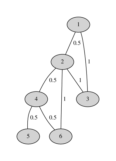
Figure 1: Sample universe graph $U$

The graph features real-valued edge labels in the $(0,1]$ interval that represent confidence weights of the edges (the higher the label the higher the expected degree of association between the corresponding vertices). These edge labels are used when constructing several auxiliary resources from the graph. There are no specific types of edges (i.e., predicates) in the examples since in the experiments reported in this article, we focus only on one type of relationship based on automatically extracted co-occurrence statements.

First of all, we need to define a metric on the vertices. The most straightforward option without any background knowledge on the graph is to use its (weighted) adjacency matrix for constructing characteristic context vectors for every vertex. The vectors can then be used for computing the actual metric.

The adjacency matrix $A_{U}$ of $U$ is presented in Table 1.

	1	2	3	4	5	6
1	0	0.5	1	0	0	0
2	0.5	0	1	0.5	0	1
3	1	1	0	0	0	0
4	0	0.5	0	0	0.5	0.5
5	0	0	0	0.5	0	0
6	0	1	0	0.5	0	0

Table 1: Weighted adjacency matrix $A_{U}$

The context vector $\mathbf{x}$ for a vertex $x$ is the row (or column, as the graph is undirected) corresponding to $x$ in the adjacency matrix $A_{U}$. Using the context vectors, we can define the Euclidean distance (i.e., a metric) on the vertices as $\delta(x,y)=\sqrt{\sum_{i=1}^{n}(x_{i}-y_{i})^{2}}$ where $x_{i},y_{i}$ correspond to the $i$-th elements of the $\mathbf{x},\mathbf{y}$ context vectors, respectively. The specific distances (up to 4-th decimal point) between the universe vertices are given in Table 2.

	1	2	3	4	5	6
1	0	1.3229	1.5	1.2247	1.2247	1.2247
2	1.3229	0	1.8708	1.5	1.5	1.8028
3	1.5	1.8708	0	1.3229	1.5	1.118
4	1.2247	1.5	1.3229	0	1	1
5	1.2247	1.5	1.5	1	0	1
6	1.2247	1.8028	1.118	1	1	0

Table 2: Distance matrix $D_{U}$

The last auxiliary structure we will need in the following sections (namely for defining complexity measures) is clustering of the vertices in $U$. An example of a possible clustering is given in Figure 2.

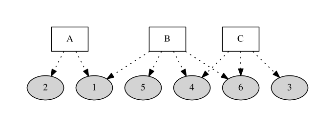
Figure 2: Cluster structure of $U$

It is an overlapping clustering that groups vertices with mutual distances below $1.5$ (in the actual implementation of our approach, we use more sophisticated clustering method as explained in detail in Section 4.2.1). The clustering contains three clusters $A:\{1,2\},B:\{1,4,5,6\},C:\{3,4,6\}$. Note that the clustering can either be computed from the universe graph itself or provided externally (e.g., in the form of an ontology that defines a taxonomy upon the graph vertices).

3.2 Measure Definitions

Having introduced the sample universe, we can continue with the specific measure definitions which we use later on in the literature-based discovery experiments.

3.2.1 Conservatism

Following the conditions provided in Section 2.2.1, we define a specific instance of the hypothesis graph conservatism measure

$$C(H)=\frac{1}{|\pi_{s}(H,\delta)|}\sum_{p\in\pi_{s}(H,\delta)}\frac{\delta(v_{1},v_{|p|})}{\sum_{i=1}^{|p|-1}\delta(v_{i},v_{i+1})},$$

where $\pi_{s}(H,\delta)$ is a set of all shortest paths in $H$ w.r.t. the Euclidean distance $\delta$ and $p=(v_{1},v_{2},\dots,v_{|p|})$ is a specific shortest path of length $|p|$. In other words, the $C$ measure is an arithmetic mean of the shortest path conservatism values where the path conservatism is computed as a fraction of the distance between the extreme vertices of the path and the path length.

The measure satisfies the condition 1. from Section 2.2.1 as it already focuses only on paths with minimal aggregate distance between the consecutive vertices (assuming the sum aggregation). The condition 2. is satisfied as well. For any path $p$, $\delta(v_{1},v_{|p|})\leq\sum_{i=1}^{|p|-1}\delta(v_{i},v_{i+1})$. The equality is achieved if and only if the context vectors of the consecutive vertices represent points that lie in a straight line, i.e., maximise the distance between the extreme vertices of the path. Therefore the maximum value $1$ of the path conservatism measures is achieved exactly when the extreme distance is maximal.

Example 1

In Figure 3 there are three hypothesis graphs $E,F,G$ that exist in the universe $U$ described in Section 3.1.

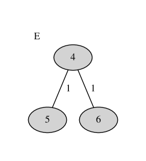
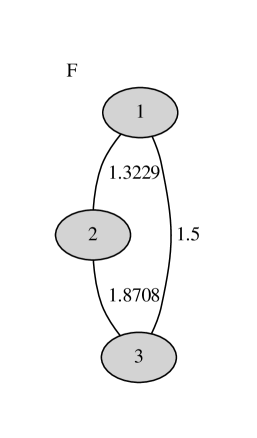
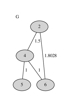
Figure 3: Sample hypothesis graphs $E,F,G$

The edges are annotated with the Euclidean distance $\delta$ based on the vertex context vectors (see the examples in Section 3.1 for details).

The numbers of all shortest paths for the hypothesis graphs $E,F,G$ w.r.t. the distance $\delta$ are $3,3,6$, respectively. The conservatism measures of the hypotheses are

$$C(E)=\frac{1}{3}(\frac{1}{1}+\frac{1}{2}+\frac{1}{1})=0.8\overline{3},$$

$$C(F)=\frac{1}{3}(\frac{1.3229}{1.3229}+\frac{1.8708}{1.8708}+\frac{1.5}{1.5})=1,$$

$$C(G)=\frac{1}{6}(\frac{1.5}{1.5}+\frac{1.8028}{1.8028}+\frac{1}{1}+\frac{1}{1}+\frac{1.5}{2.5}+\frac{1}{2})=0.85,$$

therefore the hypotheses can be ranked in the

$$F\succ_{C}G\succ_{C}E$$

order from the most to the least conservative one.

3.2.2 Modesty

As an approximation of the the ideal modesty measure presented in Section 2.2.2, we use inverse density of the hypothesis graph

$$M(H)=\frac{|V_{H}|(|V_{H}|-1)}{2|E_{H}|}.$$

This function is much easier to compute than the ideal one and is monotonic w.r.t. it. Since the enumerators of both functions are fixed, we only need to show that the number of edges is monotonic w.r.t. number of all simple paths in a hypothesis graph. This is quite easy – increase in $|E_{H}|$ (i.e., adding an edge) will cause $|\Pi(H)|$ to grow as well since adding an edge will result in at least one new simple path in $H$, the edge itself. Conversely, if the set $\Pi(H)$ grows, it means that edges had to be added to the $H$ graph as it is the only way how the overall number of paths can be increased.

Example 2

The number of edges in the $E,F,G$ graphs from Example 1 is $2,3,4$, respectively, while the maximum possible number of edges in the corresponding complete graphs is $3,3,6$. Therefore the modesty values are

$$M(E)=\frac{3}{2}=1.5,\;M(F)=\frac{3}{3}=1,\;M(G)=\frac{6}{4}=1.5$$

and the modesty ranking of the hypotheses is

$$E\succ_{M}F,\;G\succ_{M}F.$$

3.2.3 Simplicity

As stated in Section 2.2.3, we use the dual notion of complexity for measuring hypothesis simplicity. For the specific instance of the measure, we employ Shannon’s entropy that has been frequently used for graph complexity [25]. To define the entropy, we utilise the clustering of the hypothesis graph vertices based on their context vectors. Let us assume a vertex labeling $\gamma:V_{U}\rightarrow 2^{L}$ where $L$ is a set of cluster identifiers. Then we can define a cluster association probability $p(l,H)$ for a specific cluster $l\in L$ within a hypothesis $H$ as

$$p(l,H)=\frac{|\{v|v\in V_{H}\wedge l\in\gamma(v)\}|}{|V_{H}|}.$$

It is a probability that a randomly selected vertex from $H$ belongs to a cluster $l$. If we conceive clusters as higher-level topics the hypothesis graph deals with, then the probability reflects the distribution of the topics across the graph. The $p(l,H)$ values can be used for computing the cluster association entropy for a hypothesis $H$ as

$$E(H)=-\sum_{l\in L}p(l,H)\log_{2}p(l,H).$$

It reflects the information value of the hypothesis’ cluster structure – the more “unpredictably” distributed clusters, the higher the complexity and also the information value. This conforms to an intuitive assumption that hypotheses dealing with more topics representatively are more informative, i.e., complex.

We define two simplicity measures that employ the cluster association entropy and satisfy the respective conditions introduced in Section 2.2.3

$$S_{1}(H)=E(H),\;S_{2}(H)=\frac{E(U\setminus H)}{E(U)}.$$

We use both measures in the following to capture different aspects of simplicity simultaneously.

Example 3

In Figure 4 there are the three hypotheses graphs $E,F,G$ and the universe graph $U$ depicted again, but this time with cluster annotations provided as vertex labels.

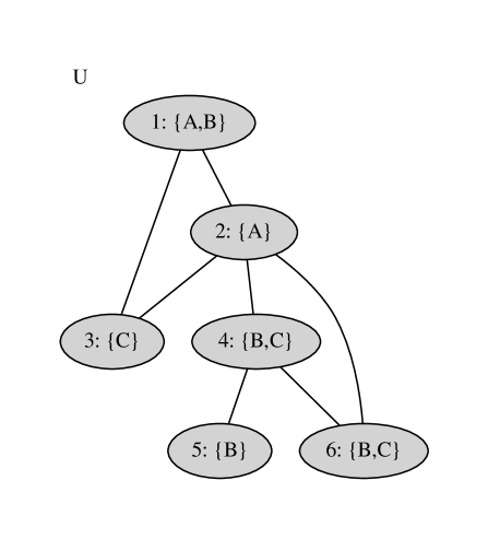
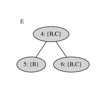
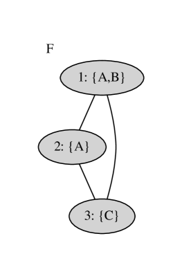
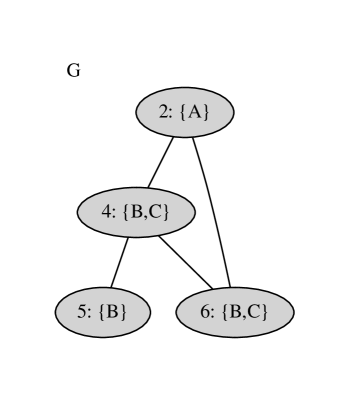
Figure 4: Sample hypothesis graphs $E,F,G$

The cluster association probabilities for each graph are

$$p(A,U)=\frac{1}{3},\;p(B,U)=\frac{2}{3},\;p(C,U)=\frac{1}{2},$$

$$p(A,E)=0,\;p(B,E)=1,\;p(C,E)=\frac{2}{3},$$

$$p(A,F)=\frac{2}{3},\;p(B,F)=\frac{1}{3},\;p(C,F)=\frac{1}{3},$$

$$p(A,G)=\frac{1}{4},\;p(B,G)=\frac{3}{4},\;p(C,G)=\frac{1}{4}.$$

The entropies corresponding to these probabilities are

$$E(U)\doteq 1.4183,\;E(E)\doteq 0.39,\;E(F)\doteq 2.78,\;E(G)\doteq 1.3113,$$

$$E(U\setminus E)\doteq 2.78,E(U\setminus F)\doteq 0.39,E(U\setminus G)=1.5.$$

The hypothesis $F$ is the lowest-ranking no matter which function we use – it has the lowest entropy and $E(U\setminus F)<E(U)$, therefore it makes the universe more complex. On the other hand, both $E,G$ increase the simplicity of the universe. If only local complexity of the acceptable hypotheses is relevant (measure $S1$), then the final ranking is

$$G\succ_{S1}E\succ_{S1}F$$

since $E(G)>E(E)$. However, if the rate of simplifying the universe is more important (measure $S2$), the ranking is

$$E\succ_{S2}G\succ_{S2}F$$

as

$$\frac{E(U\setminus E)}{E(U)}\doteq 1.9601>1.0576\doteq\frac{E(U\setminus G)}{E(U)}.$$

3.2.4 Generality

To limit the potentially intractable number of paths in the ideal generality formula introduced in Section 2.2.4, we apply two approximations in its specification. Firstly, we focus only on explanations for the universe vertices $V_{A}^{H}$ that are immediately adjacent to the measured hypothesis $H$. The set of edges that connect these vertices to $H$ can then be defined as $E_{A}^{H}=\{(u,v)|(u,v)\in E_{U}\wedge(u\in V_{A}^{H},v\in V_{H}\vee u\in V_{H},v\in V_{A}^{H})\}$. The second approximation consists of focusing only on shortest paths w.r.t. the $\delta$ distance. The specific generality measure is then defined as

$$G(H)=|\{p|p\in\pi_{s}(U,\delta)\wedge p_{1}\in V_{A}^{H}\wedge p_{2},p_{3},\dots,p_{|p|}\in V_{H}\}|.$$

The measure corresponds to the number of shortest paths that start in an adjacent vertex and connect it with vertices in the hypothesis graph $H$, thus providing an explanation for it using only $H$. As the graphs $H$ are assumed to be connected, the measure can further be simplified as $G(H)=|E_{A}^{H}|(1+(V_{H}-1))=|E_{A}^{H}||V_{H}|$ for graphs where only one shortest path exists between any two vertices.

The $G(H)$ measure uses sum aggregation as the $g$ function present in the general definition. The $f$ function that leads to the presented definition of $G(H)$ returns zero for any vertex from the $V_{U}\setminus V_{H}$ set that is not immediately adjacent to $H$. For other vertices, it returns the number of paths that provide explanation for them in $H$. This number is positively correlated with the number of vertices in $V_{H}$ as required in the general definition, since the number of paths leading from a vertex to other vertices in a connected graph $H$ is $|V_{H}|-1$ (or more if multiple shortest paths exist between some vertices).

The restriction to the immediately adjacent vertices leads to a narrowly focused generality and helps to reduce combinatorial explosion resulting from taking the whole universe graph into account. The shortest path approximation is a reasonable limitation as these paths are more likely to be conservative explanations. It is not strictly monotonic w.r.t. the ideal generality measure, though. If the number of shortest paths increases, then the number of all paths naturally has to be higher as well. The other direction is less obvious, and conditional. Assuming the number of all paths in a graph has increased, we have to show that there also has to be more shortest paths. This is not true in general – if edges between distant vertices are added, they may not contribute to increasing the number of shortest paths. However, since the measure intuitively captures the notion of generality in the context of knowledge graphs and is easy to compute, we decided to relax the absolute monotonicity requirement for the sake of practicality.

Example 4

The sets vertices adjacent to the $E,F,G$ hypotheses are

$$V_{A}^{E}=\{2\},\;V_{A}^{F}=\{4,6\},V_{A}^{G}=\{1,3\}$$

and the corresponding sets of connecting edges are

$$E_{A}^{E}=E_{A}^{F}=\{(4,2),(6,2)\},\;E_{A}^{G}=\{(2,1),(2,3)\}.$$

Since there is only one shortest path between any pair of vertices in our example, the generality measures are

$$G(E)=|E_{A}^{E}|\cdot|V_{E}|=2\cdot 3=6,\;G(F)=|E_{A}^{F}|\cdot|V_{F}|=2\cdot 3=6,\;$$

$$G(G)=|E_{A}^{G}|\cdot|V_{G}|=2\cdot 4=8$$

and the resulting ranking is

$$G\succ_{G}E,\;G\succ_{G}F.$$

3.2.5 Refutability

Using the shortest paths approximation again, we define a specific refutability measure as

$$R_{k}(H)=\frac{|\pi_{s}(H,\delta)|}{|\pi_{s}(H,\delta)|+\sum_{i=1}^{k}|\pi_{s}(H/R(i),\delta)|}.$$

Similarly to Section 3.2.4, we consider only the shortest paths instead of all simple ones, which makes the computation of the measure comparatively easier. Such an approximation is unfortunately not strictly monotonic as shown before, however, we believe that the practicality and intuitiveness of the measure outweighs the partial monotonicity violation.

For the ranking $R$ of the vertices in the $R_{k}(H)$ measure computation, we use the betweenness centrality which is defined as

$$c_{B}(v,G)=\frac{|\{p|p\in\pi_{s}(G,\delta)\wedge v\in p\}|}{|\pi_{s}(G,\delta)|},$$

where $v$ is a vertex and $G$ is a graph. In other words, betweenness centrality of a vertex is the number of shortest paths passing though it divided by total number of shortest paths. The ranking $R$ ranks the vertices in a decreasing order based on their betweenness centrality. Such ranking generally does not mean that removal of a high-ranking vertex results in a higher number of shortest paths disappearing when compared to a removal of a lower-ranking vertex – if the graph remains connected in both cases, the number of shortest paths in it will be the same after removal of either node. However, removing a vertex with higher betweenness centrality will result in relative increase of the remaining paths’ lengths. This can lead to a decrease of the graph conservatism and thus also to a decrease of its overall value w.r.t. the hypothesis virtues. Consequently, making a hypothesis weaker more quickly can be seen as refuting it more efficiently. We believe that this justifies the chosen ranking even though it means yet another relaxation of the general requirements.

Example 5

The sets of shortest paths w.r.t. the $\delta$ distance for the particular hypothesis graphs are

$$\pi_{s}(E,\delta)=\{(5,4),(5,4,6),(4,6)\},$$

$$\pi_{s}(F,\delta)=\{(2,1),(2,3),(1,3)\},$$

$$\pi_{s}(G,\delta)=\{(2,4),(2,4,5),(2,6),(4,5),(4,6),(5,4,6)\}.$$

The corresponding vertex betweenness centralities are then

$$c_{B}(4,E)=1,\;c_{B}(5,E)=c_{B}(6,E)=0.\overline{6},$$

$$c_{B}(1,F)=c_{B}(2,F)=c_{B}(3,F)=0.\overline{6},$$

$$c_{B}(2,G)=c_{B}(5,G)=c_{B}(6,G)=0.5,\;c_{B}(4,G)=0.8\overline{3}.$$

The top-1 refutability measure for the hypothesis $E$ can be computed as follows. The centrality-based ranking of the vertices places $4$ on the top, therefore we remove it. The result is a disconnected graph consisting of isolated vertices $5,6$ where no path exists anymore. The top-1 refutability measure of $E$ is thus

$$R(E,1)=\frac{3}{3+0}=1.$$

Similarly, the top-1 refutability measures for the remaining two hypotheses (with arbitrary removal vertex selection for $F$ due to uniform centrality ranking) are

$$R(F,1)=\frac{3}{3+1}=0.75,\;R(G,1)=\frac{6}{6+1}=0.\overline{857142}.$$

The resulting refutability ranking of $E,F,G$ is

$$E\succ_{R}G\succ_{R}F.$$

3.3 Combining the Measures

The specific measures defined in the previous section can be used to rank the hypothesis graphs independently of each other as shown in the examples. However, practical applications will very often imply the necessity to compare hypotheses along all the measures. Lacking any a priori information on which measures may be more relevant for a particular application, we propose the following way of ordering the hypothesis graphs.

Let $\mathcal{H}=\{H_{1},H_{2},\dots,H_{n}\}$ be the set of hypothesis graphs we wish to compare according to a set of measures $\mathcal{X}=\{X_{1},X_{2},\dots,X_{m}\}$ of equal importance. Then we can construct an edge-labeled directed ranking multigraph $\mathcal{R}=(\mathcal{H},\mathcal{E}\subseteq\mathcal{H}\times\mathcal{H},\lambda:\mathcal{E}\rightarrow\mathcal{X})$. The multigraph’s vertices are the hypotheses in $\mathcal{H}$. The edge set and the labeling function is constructed from the specific measure rankings so that $(H_{i},H_{j})\in\mathcal{E},\lambda(H_{i},H_{j})=X_{k}$ if and only if there is a measure $X_{k}$ such that $H_{i}\succ_{X_{k}}H_{j}$. Using the ranking multigraph $\mathcal{R}$, we can define a combined ranking relation $\succ$ on the set $\mathcal{H}\times\mathcal{H}$ as

$$H_{i}\succ H_{j}\mathrm{\;if\;and\;only\;if\;}\frac{d_{o}(H_{i},\mathcal{R})}{d_{o}(H_{i},\mathcal{R})+d_{i}(H_{i},\mathcal{R})}>\frac{d_{o}(H_{j},\mathcal{R})}{d_{o}(H_{j},\mathcal{R})+d_{i}(H_{j},\mathcal{R})},$$

where $d_{i}(H_{x},\mathcal{R}),d_{o}(H_{x},\mathcal{R})$ is the in-degree and out-degree of the vertex $H_{x}$ in the multigraph $\mathcal{R}$, respectively. In plain words, the combined ranking relation $\succ$ orders the hypotheses based on the relative magnitude of their superiority (out-degree) w.r.t. the specific ranking relations given by the measures.

Example 6

Figure 5 shows the ranking multigraph corresponding to Examples 1-5.

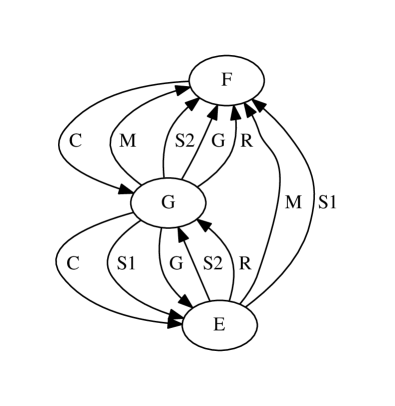
Figure 5: Ranking multigraph for $E,F,G$

A directed edge from vertex $X$ to $Y$ with a label $Z$ means that $X\succ_{Z}Y$. The in-degrees and out-degrees of $E,F,G$ in the ranking graph are

$$d_{i}(E)=3,\;d_{o}(E)=4,\;d_{i}(F)=6,\;d_{o}(F)=1,\;d_{i}(G)=3,\;d_{o}(G)=7,$$

therefore

$$G\succ E\succ F$$

since

$$\frac{7}{10}>\frac{4}{7}>\frac{1}{7}.$$

4 Experimental Validation

In order to validate the proposed formalisation of hypothesis virtues in the context of knowledge graphs, we chose to follow-up on our work presented in [30] where we addressed automated extraction of conceptual networks from biomedical literature. The work deals with extraction of co-occurrence and similarity relationships from abstracts available on PubMed (c.f., http://www.ncbi.nlm.nih.gov/pubmed) and consequent indexing, querying and navigation of the networks in a knowledge discovery scenario.

As we have shown in [30], the automatically extracted networks can already provide useful insights even for experts in the field, however, they still contain some noise and irrelevant and/or obvious information. Tackling this challenge has been the main practical motivation for the research presented in this article. We believe we can use our approach to identify portions of the automatically extracted graphs that can not only provide general overview of the domain with less noise, but also isolate valid relationships that are surprising for experts. This can ultimately lead to more efficient machine-aided discovery applications.

In our validation experiments, we utilise the scenarios, data sets and evaluation methodologies elaborated within the field of literature-based discovery which we introduce in Section 4.1 below. Section 4.2 is the methodological core of this part. It presents an evolutionary approach to the refinement of automatically extracted knowledge graphs using the hypothesis virtue measures. Section 4.3 describes the data sets and methods we use for the experimental evaluation. Finally, Section 4.4 discusses the results of the experiments.

Note that we have implemented our approach and the experiments reported in this section using a Python prototype available under the GPL free software license. The corresponding code, experimental data and results are available at http://skimmr.org/hyperkraph/. Detailed README documentation on the implementation and data is provided as a part of the respective archives hosted at the referenced URL.

4.1 Literature-Based Discovery

The field of literature-based discovery is widely considered to stem from the work [44]. Based on [44] and a follow-up article [45], the work [43] introduced the notion of Swanson linking – connecting two pieces of knowledge in isolated documents A and B using concepts from intermediate documents (C) that are directly or indirectly related to A and B. Surveys of recent works addressing this problem are provided in [7, 34, 41].

The application of our framework to refining knowledge graphs automatically extracted from literature is closely related to literature-based discovery. Our goal is to generate a set of graphs that reflect relationships between terms in literature and are optimised w.r.t. hypothesis virtues. Such a structure can very straightforwardly facilitate the process of finding “interesting” links between isolated concepts via intermediates, which is the key problem of literature discovery. Therefore we can use the standard approaches and man-made “gold standard” discoveries from that field to experimentally validate our approach in an established application scenario.

4.2 Evolutionary Refinement of Automatically Extracted Knowledge Graphs

The basic assumption we use for validating our framework is that applying the hypothesis virtue measures to refining graphs extracted from literature will facilitate literature-based discovery tasks better than the unrefined graphs. To verify this, we have to tackle the graph refinement first. The key question is: Given a knowledge graph based on statements automatically extracted from text, how can we refine it so that only the parts of the graph that have comparatively high hypothesis virtue measures remain?

This is essentially an optimisation problem in which we know how to tell whether a solution X is better than Y, but we do not know much about what the actual solutions are and how the main knowledge graph is (or should be) composed of them. Such problems can quite efficiently be tackled by evolutionary computing [9]. In the rest of this section, we describe a specific algorithm for evolutionary refinement of knowledge graphs.

4.2.1 Extracting a Universe Graph from Texts

Figure 6 presents the high-level overview of the graph extraction and refinement process.

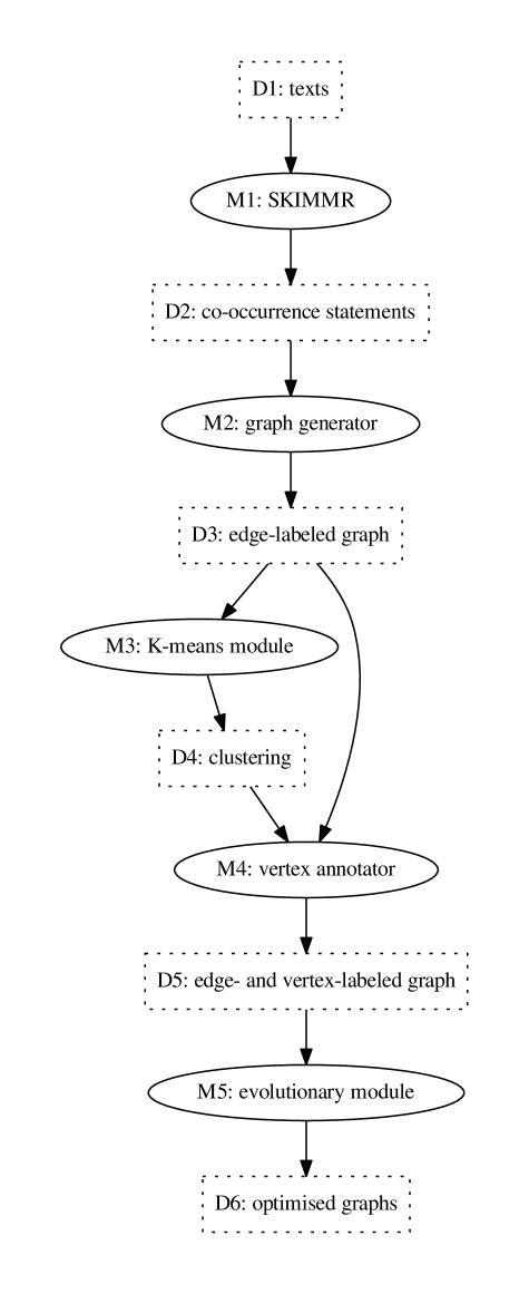
Figure 6: High-level workflow of the graph construction and refinement

First we use our SKIMMR tool [30] to extract basic co-occurrence statements from the input texts. The statements are in the shape of tuples $(t_{1},t_{2},w_{d},T)$, where $t_{1},t_{2}$ are two terms that co-occur in an input text $T$ and $w_{d}$ is the weight of the co-occurrence based on the sentence distances of the terms within $T$.

In the next step (M2 in Figure 6), we:

1. Use the basic statements to compute corpus-wide co-occurrence weights using normalised point-wise mutual information.

2. Encode the terms in the statements using integer identifiers (to optimise the memory usage in the consequent steps).

3. Build a fulltext index upon the lexical vertex labels for accessing them during the evaluation (this mitigates the impact of spelling alternatives and other irregularities in the automatically extracted names).

4. Initialise an undirected edge-labeled universe graph $U$ with edges constructed from the corpus-wide statements. The graph can possibly be limited to edges with normalised point-wise mutual information weights above a pre-defined threshold.

5. Construct a context vector space for the $U$ vertices based on their neighbors and corresponding edge weights.

6. Use the vector space to compute the Euclidean distances between the vertices.

Steps M3 and M4 in Figure 6 perform the K-means clustering of the universe graph $U$ in order to provide a vertex labeling $\gamma$ that associates each vertex with cluster(s) it belongs to (see Section 4.3.3 for details on the K-means settings in the particular experiments we conducted). At this moment, everything is ready for optimising $U$ according to the hypothesis virtue measures of its sub-graphs.

4.2.2 Evolutionary Graph Refinement

The optimisation step in Figure 6 is performed using a genetic algorithm [9]. Its detailed workflow is presented in Figure 7.

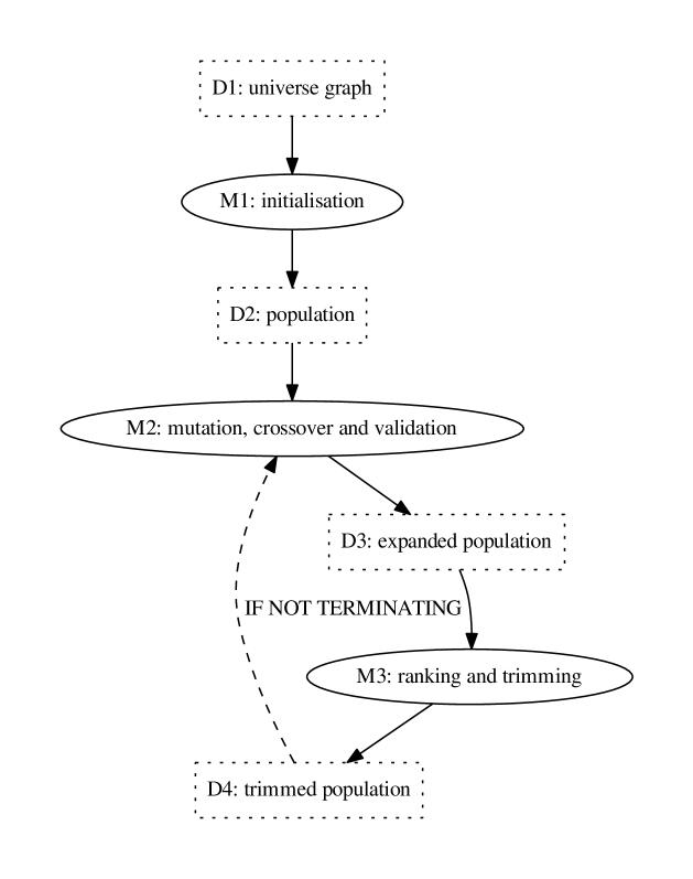
Figure 7: Detailed workflow of the evolutionary refinement

The genetic algorithm has the following configurable parameters: 1. mutation and mating probabilities $p_{m},p_{c}$ defining how likely it is for an individual in a population to mutate and mate (i.e., engage in a crossover with another individual); 2. number $k_{m}$ defining how many times an individual can attempt to mate in a generation; 3. maximum number of generations $N_{G}$; 4. rate $\rho_{p}$ of the standard deviation of the population size – it sets the size of the population $P_{i}$ to $|P_{i}|=gauss(|P_{i-1}|,\rho_{p}|P_{i-1}|)$ where $gauss(\mu,\sigma)$ returns a random number from the normal distribution with mean $\mu$ and standard deviation $\sigma$, truncated to integer; 5. the mean and standard deviation $\mu_{i},\sigma_{i}$ for determining the sizes of the individuals in the initial population. For specific values of the parameters and discussion of their influence on the evolution process in our experiments, see Section 4.3.3.

The population is initialised (step M1 in Figure 7) by a repetitive random selection of possibly overlapping stars of size $gauss(\mu_{i},\sigma_{i})$ from the graph $U$. Stars consist of one “hub” vertex and a set of vertices “fanning out” of the hub via immediate edges. They are a specific type of sub-graphs that can be used as atomic graph construction blocks [25] and thus they are fitting for the purpose of population initialisation.

Step M2 in Figure 7 consists of applying the evolutionary operators on the population and consequent validation of the newly added individuals which discards disconnected ones. The mutation deletes or adds an edge from/to the individual graph with equal probabilities. The crossover combines two parents by randomly selecting half of the edges from each parent and combining them in a new individual. All existing edge labels are copied in the process of creating new individuals.

Step M3 in Figure 7 is essential for the optimisation – it computes the hypothesis virtue measures of each individual in the expanded population and then ranks the population according to the combined ranking $\succ$ introduced in Section 3.3. The population is then trimmed to a random size based on the previous population size (computed using the $\rho_{p}$ parameter).

Steps M2 and M3 are repeated until a termination condition is met. This can either be reaching a pre-defined number of generations $N_{G}$, or achieving some sort of population convergence.

4.3 Description of the Experiments

For the evaluation of our approach we chose two standard scenarios in literature-based discovery based on the works [44, 45]. Details on the corresponding data sets and experiments we performed using them are described in the following sections.

4.3.1 Data Acquisition

We used two data sets in the experimental evaluation, both of which address discovery of connections between previously isolated concepts (and corresponding bodies of literature). One data set is based on [44] that explores the relationship between fish oil and Raynaud’s syndrome. The other data set is based on similar study of previously neglected connections between migraine and magnesium [45]. We refer to these two data sets and corresponding experiments as to $T_{R},T_{M}$, respectively.

The initial corpora of texts for the $T_{R},T_{M}$ experiments were obtained from PubMed via queries compiled according to the specifications given in [44, 45]. Each of these works defines source and target terms $t_{s},t_{t}$ together with a set $I_{c}$ of intermediate terms that connect them. A query for the PubMed abstracts corresponding to specific $t_{s},t_{t},I_{c}$ is compiled as a disjunction of atomic conjunctions

$$\bigvee_{t\in\{t_{s},t_{t}\},t_{c}\in I_{c}}(t\wedge t_{c})$$

The particular queries we used for obtaining the $T_{R},T_{M}$ corpora were

("raynaud" AND "blood") OR ("raynaud" AND "viscosity") OR
("raynaud" AND "platelet") OR ("raynaud" AND "vascular") OR
("raynaud" AND "reactivity") OR ("fish oil" AND "blood") OR
("fish oil" AND "viscosity") OR ("fish oil" AND "platelet") OR
("fish oil" AND "vascular") OR ("fish oil" AND "reactivity")

and

("migraine" AND "vasospasm") OR ("migraine" AND "spreading depression") OR ("migraine" AND "vascular reactivity") OR ("migraine" AND "depolarization") OR ("migraine" AND "epilepsy") OR ("migraine" AND "inflammation") OR ("migraine" AND "prostaglandins") OR
("migraine" AND "platelet aggregation") OR ("migraine" AND "serotonin") OR ("migraine" AND "brain anoxia") OR ("migraine" AND "calcium channel blockers") OR ("magnesium" AND "vasospasm") OR ("magnesium" AND "spreading depression") OR ("magnesium" AND "vascular reactivity") OR ("magnesium" AND "depolarization") OR ("magnesium" AND "epilepsy") OR ("magnesium" AND "inflammation") OR ("magnesium" AND "prostaglandins") OR ("magnesium" AND "platelet aggregation") OR ("magnesium" AND "serotonin") OR ("magnesium" AND "brain anoxia") OR ("magnesium" AND "calcium channel blockers")

respectively. Note that the while the $T_{M}$ query exactly corresponds to the terms given in [45], the $T_{R}$ query is relaxed to sub-terms as the exact query only yields very few abstracts. The PubMed search was limited to articles indexed until November, 1985 and August, 1987 for $T_{R},T_{M}$, respectively, so that we can compare ourselves to the findings of the original works which have served as a de facto gold standard in the literature-based discovery field [4].

The characteristics of the $T_{R},T_{M}$ corpora are summarised in Table 3.

Corpus	# of abstracts	# of tokens	# of base statements
$T_{R}$	1,406	90,427	407,154
$T_{M}$	3,611	319,810	1,534,685

Table 3: Basic statistics of the corpora

Number of tokens is a sum of the word-length of the documents in the corpus and number of base statements is the number of the base co-occurrence statements the SKIMMR tool extracted from the corpus.

4.3.2 Graph Extraction

To generate knowledge graphs from the text corpora, we use the approach introduced in Section 4.2. We construct the experimental graphs using only co-occurrence statements with above-average positive normalised point-wise mutual information scores. This filters out statements with comparatively low co-occurrence weight. We use the general SKIMMR version that extracts entities based on shallow parsing rather than domain-specific models (see https://github.com/vitnov/SKIMMR for details). This is to demonstrate the generality of our work – if we show that our approach can deliver good results even in quite a specific domain using basic and universally applicable initial text mining, it indicates that it is likely to perform similarly well in any other domain.

The characteristics of the extracted graphs are provided in Tables 4 and 5.

Graph	$|V_{G}|$	$|E_{G}|$	$dn_{G}$	$|C_{G}|$	$|c_{G}^{max}|$	$|c_{G}^{avg}|$	$|c_{G}^{med}|$
$T_{R}$	16,714	181,140	1.297e-3	80	16,497	208.925	2
$T_{M}$	52,681	635,705	4.581e-4	110	52,373	478.918	2

Table 4: Basic characteristics of the experimental graphs

The basic characteristics $|V_{G}|,|E_{G}|,dn_{G},|C_{G}|,|c_{G}^{max}|,|c_{G}^{avg}|,|c_{G}^{med}|$ in Table 4 are the number of vertices, number of edges, graph density, number of connected components, maximum, average and median component size in vertices, respectively. The component-wise characteristics in Table 5 are computed as a weighed arithmetic mean across all the components where the weight is the component size in vertices.

Graph	$rd_{G}$	$dm_{G}$	$tr_{G}$	$asp_{G}$	$asp_{G}^{\delta}$
$T_{R}$	5.935	8.897	0.397	4.045	6.956
$T_{M}$	5.971	8.954	0.259	3.964	7.702

Table 5: Component-wise characteristics of the experimental graphs

The characteristics $rd_{G},dm_{G}$ are the graph radius and diameter (minimum and maximum eccentricity, respectively, where eccentricity of a vertex is its maximum distance to other vertices). The $tr_{G}$ characteristics is transitivity – the fraction of all possible triangles reflecting the tendency of vertices in the graph to cluster together [39]. The characteristics $asp_{G},asp_{G}^{\delta}$ are average shortest path lengths in terms of edges and the distance labeling, respectively. Additional characteristics of the graph is the degree distribution depicted in Figure 8 (the plot is log-scaled in both x- and y-axis).

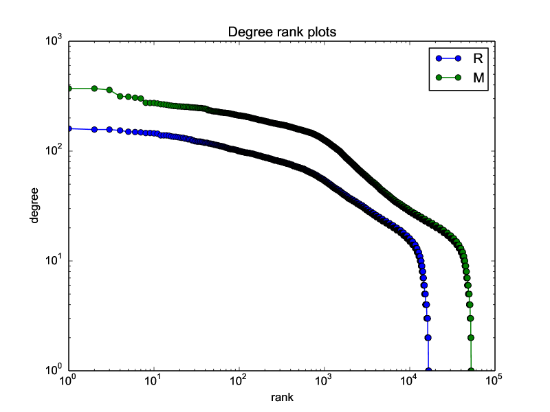
Figure 8: Degree distributions for the experimental graphs

The extracted graphs both have one large connected component comprising most of the vertices, complemented by other trivial components mostly consisting of one edge. The largest components exhibit so called “small-world” property [48] – despite of being quite large and having small density, they have relatively small diameters and average shortest paths. This observation is supported by two additional facts. The graphs have relatively high transitivity, i.e., high tendency of vertices to cluster together which is typical for complex small-world networks [39]. Also, the vertex degree distribution approximately follows the power law as shown in Figure 8, which is characteristic for scale-free networks [31]. This means that the extracted graphs have relatively densely connected structure with many claims involving frequently repeated concepts, which is largely caused by highly (co)occurring terms. This is perhaps not ideal for making discoveries about as many previously disconnected phenomena as possible, and we later show how our approach can remedy this problem.

4.3.3 Settings of the Clustering and Evolutionary Refinement Algorithms

For the clustering, we use the K-means module of the scikit-learn package [32]. As the algorithm’s scalability to large numbers of samples and features is limited by available memory, we partition the set of context vectors corresponding to the universe graph vertices to buckets of size $2,000$ and then run the K-means algorithm on them with the parameter $K$ set to $40$. The partitioning is done by incremental random selection of $50$ seed vectors from the unpartitioned set, computing their centroid and then filling the partition with the seeds plus up to $1,950$ unpartitioned vectors closest to the centroid. We have experimented with different settings of every parameter, however, we found out that the resulting distributions of vectors into clusters are practically invariant to the settings, with mean and median cluster sizes converging to the same values no matter what the settings were.

The parameters of the evolutionary refinement were

$$p_{m}=0.05,p_{c}=0.75,k_{m}=5,N_{G}=50,\rho_{p}=0.05,\mu_{i}=100,\sigma_{i}=80.$$

The initial individual size parameters are only reflected in rare extreme cases as the size of the random stars is much more dependent on the data set structure in practice. For the other parameters, we applied values typically used by model approaches presented in the evolutionary computing literature [9]. The number of generations has been set well above a threshold after which the performance of the corresponding populations starts to oscillate around similar evaluation scores (see Section 4.4.1 for details).

The evolutionary refinement with these parameters took 56m and 6h36m for the $T_{R},T_{M}$ experiments, respectively, using a 2010 make laptop with 4-core CPU, 8GB RAM and Ubuntu Linux 14.04 OS. The virtue measures (the most demanding part) were computed using six parallel processes. The number of processes can be easily adjusted to the computing power available, which facilitates vertical scalability of the refinement. Horizontal scalability is planned for future versions of the prototype and consists of using a distributed processing library instead of the native Python multiprocessing module.

4.3.4 Evaluation Methodology

We use several evaluation methods. Part of them is based on a recent work [4] which defines evidence-based and literature frequency-based evaluation measures within the de facto standard literature-based discovery scenarios elaborated in [44, 45]. The additional benefit of using [4] as a primary reference for the evaluation is that the authors compared results of several representative approaches to literature-based discovery. Thus we can interpret our results within a broader context of the whole field. In addition to the measures defined in [4], we perform qualitative evaluation of the actual contents of the results and compare ourselves to related state of the art where applicable.

The evidence-based evaluation measures the capability of an approach to re-discover the intermediate concepts linking the source and target in the corpus as per discoveries made by human experts. It also measures the importance the approach associates with the re-discovery. For an intermediate $t_{c}$, the absolute evidence-based evaluation measure directly corresponding to [4] is defined as

$$evd(t_{c})=\min_{G\in\mathcal{G}_{c}}(rnk(G)),$$

where $\mathcal{G}_{c}=\{G|t_{s},t_{t},t_{c}\in V_{G}\wedge\exists p\in\Pi(G).p=(t_{s},\dots,t_{c},\dots,t_{t})\}$ is a set of solution graphs that contain the source and target terms $t_{s},t_{t}$ linked by the intermediate $t_{c}$. The function $rnk:\mathcal{G}\rightarrow\mathbb{N}$ is a ranking of all solution graphs $\mathcal{G}=\{G|t_{s},t_{t}\in V_{G}\}$ from the most to the least relevant where the relevance is determined by the specific approach being evaluated.

We construct the sets of ranked solution graphs from the set of individuals in a selected refined generation by: 1. Creating a union graph from all population individuals. 2. Generating a set of paths between the source and target term vertices that also contain an intermediate vertex. 3. Ranking the paths using their hypothesis virtue measures, i.e., the $\succ$ relation, with the population union graph as a universe. The step 2. can either compute all simple paths or all shortest paths. In our experiments, we use the latter option due to tractability issues. The conception of paths as solution graphs represents another design choice consistent with the previous definitions – a path linking certain concepts is the simplest way of claiming (and potentially also explaining) something about them.

In addition to the absolute $evd$ score, we compute the overall relative importance of an intermediate term $t_{c}$. This measure is defined as a mean relative inverse rank of the graphs that contain $t_{c}$ among all solutions, i.e.,

$$evd^{r}(t_{c})=\frac{1}{|\mathcal{G}_{c}|}\sum_{G\in\mathcal{G}}\frac{|\mathcal{G}|-rnk(G)+1}{|\mathcal{G}|}.$$

It effectively measures the average relative relevance of the hypotheses linking the source and target terms via $t_{c}$ – the more often the link is discovered in high-ranking graphs, the higher the measure.

The second evaluation method proposed in [4] measures the frequency of the discovered claims in the scientific literature. Similarly to our definition, a path in the result graph is considered a claim in [4]. The literature frequency can be used to define a measure of solution rarity as

$$rar(\mathcal{G})=\frac{1}{|\pi_{s}(\mathcal{G}_{I})|}\sum_{p\in\pi_{s}(\mathcal{G}_{I})}f_{pm}(Q_{A}(p)),$$

where $\mathcal{G}_{I}=\{G|G\in\mathcal{G}\wedge\exists t_{c}\in I_{c},p\in\Pi(G).p=(t_{s},\dots,t_{c},\dots,t_{t})\}$ is a set of solutions that contain an intermediate term, $\pi_{s}(\mathcal{G}_{I})=\bigcup_{G\in\mathcal{G}}\pi_{s}(G)$ is the union of shortest paths taken across $\mathcal{G}_{I}$, and $f_{pm}$ is the number of results returned by PubMed for an association query $Q_{A}(p)$. The query for a path $(p_{1},p_{2},\dots,p_{|p|})$ corresponds to the conjunction $\bigwedge_{t\in p}t$ of all terms in the path (with a publication time window limited according to the corresponding experimental corpus). For instance, the path (fish oil, platelet aggregation, Raynaud’s syndrome) corresponds to the PubMed query "fish oil" AND "platelet aggregation" AND "Raynaud’s syndrome" AND ("0001/01/01"[PDAT] : "1985/11/30"[PDAT]) in the $T_{R}$ experiment. Finally, the rarity measure can be straightforwardly used for defining an interestingness measure [4] as a normalised inverse of the rarity

$$int(\mathcal{G})=\frac{1}{1+rar(\mathcal{G})}.$$

The qualitative evaluation of the results is based on the sets of topics covered by the particular solutions. A topic is informally defined by potentially relevant terms that lay on a path between source and target concepts in a solution. Potentially relevant terms are those that refer to non-trivial concepts that may elucidate the meaning of the particular path. Using the notion of topics, we define the measures of topical density, relative topical relevance and relative topical novelty, respectively, as

$$top_{d}(\mathcal{G})=\frac{|T_{unq}(\mathcal{G}_{I})|}{|T_{all}(\mathcal{G}_{I})|},\;top_{r}(\mathcal{G})=\frac{|T_{rel}(\mathcal{G}_{I})|}{|T_{unq}(\mathcal{G}_{I})|},\;top_{n}(\mathcal{G})=\frac{|T_{nvl}(\mathcal{G}_{I})|}{|T_{rel}(\mathcal{G}_{I})|}$$

for a set $\mathcal{G}$ of all solution graphs. The sets $T_{unq}(\mathcal{G}_{I}),T_{all}(\mathcal{G}_{I}),T_{rel}(\mathcal{G}_{I}),T_{nvl}(\mathcal{G}_{I})$ are sets of unique, all, relevant and novel topics covered by the solution graphs in $\mathcal{G}$ that contain an intermediate term.

The relevance of topics is determined by a review of the available scientific literature. This tells us whether or not a given set of terms can provide a meaningful and non-trivial explanation of the connection between the source and target terms. More specifically, a topic is considered relevant if and only if the following conditions are met simultaneously: 1. The terms in the topic refer to features of a biomedically relevant relationship that can be traced in literature. 2. The relationship is associated with the corresponding target, source and intermediate terms. 3. The relationship is not trivial – it has to be a supported by genuine discoveries presented in literature, not statements of obvious merely occurring in articles.

A novel topic is one that is relevant and not covered by any single published work in its whole. This can be determined using a publication search engine such as PubMed, where we can check the number of results of a conjunctive query involving all terms in the corresponding claim path. If the number of results is zero, then the topic is unique.

We compute the $top_{d},\;top_{r},\;top_{n}$ scores for the initially extracted and refined graphs in both experiments, focusing on solutions involving corresponding source, target and intermediate terms. Whenever applicable, we compare the relevant topics we generated with the topics (re)discovered by related approaches.

4.4 Results and Discussion

We split this section into three parts – first we explain the process of selection of the refined graphs to be evaluated, then we analyse properties of the selected graphs, and finally we discuss the results of the evaluation.

4.4.1 Selection of the Refined Graphs

Before analysing the actual results of the evolutionary refinement, we have to select the generation we will focus on. A natural criterion for that is the performance of generations in terms of the evaluation measures. The relative ranking of intermediate concepts (i.e., the $evd^{r}$ measure) is best suited for this task as it tells us to which extent the generations tend to “consider” the intermediate connections important. Figure 9 shows how the mean $evd^{r}$ values for all intermediates evolve throughout the generations for each experiment.

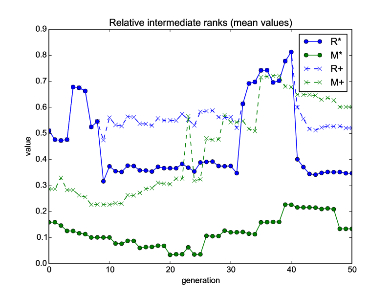
Figure 9: Mean relative intermediate ranks through generations

The blue and green lines represent the $T_{R},T_{M}$ experiments, respectively. The full lines correspond to mean values taken across all intermediate terms (also marked by the “star” character in the plot legend). The dashed lines are for mean values omitting intermediates that are not present in the given generation (marked by the “plus” character in the legend).

For the $T_{R}$ experiment, the generation 40 clearly performs best as it contains solution graphs for each intermediate term and their mean relative ranking is very high (within the top 20% of solutions). For the $T_{M}$ experiment, the situation is less clear. The best generation in terms of mean across all intermediate terms is number 39, however, if one takes only the present intermediates into account, the generations 35-38 all perform better. Yet we decided to further analyse the generation 39 as it covers three intermediates, while the generations 35-38 only cover two. From here on, we refer to the selected generations by the $T_{R}^{40},T_{M}^{39}$ expressions, respectively.

Further support for selecting the generation to be analysed can be drawn from the numbers of claims containing the source and target claims, and the numbers of such claims that also contain an intermediate term. The evolution of these values is depicted in Figure 10.

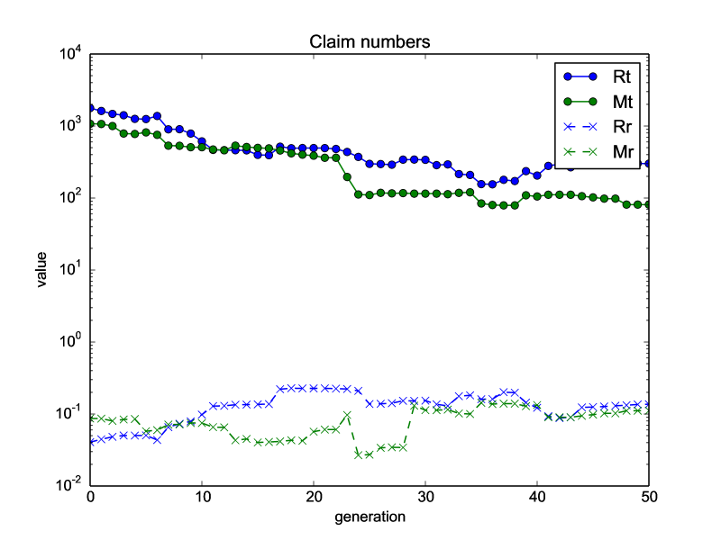
Figure 10: Claim numbers through generations

Note that the figure’s y-axis is log-scaled due to different orders of magnitude of the displayed values. Similarly to the previous figure, the blue and green lines represent the $T_{R},T_{M}$ experiments, respectively. The full lines correspond to the total number of claims containing the source and target term in a given generation (also marked by the “t” character in the plot legend). The dashed lines represent the fraction of the claims that also contain an intermediate term (marked by the “r” character).

The total number of relevant claims is steadily decreasing up until approximately 20-25th generation and then starts to oscillate. For the relative number of solutions with intermediates, similar trend can be seen after the 40-th generation. This can be interpreted as an indication that the generations are structurally stabilised then, at least for the evaluation data we work with.

4.4.2 Properties of the Refined Graphs

Before we proceed with discussing the results, let us have a look at the characteristics of the knowledge graphs corresponding to the generations we selected for evaluation. Tables 6 and 7 present the same type of data like the tables in Section 4.3.2. The extra rows with the $\Delta$ prefixes show the relative difference between the refined and initial graphs.

Graph	$|V_{G}|$	$|E_{G}|$	$dn_{G}$	$|C_{G}|$	$|c_{G}^{max}|$	$|c_{G}^{avg}|$	$|c_{G}^{med}|$
$T_{R}^{40}$	10,879	15,940	2.694e-4	81	10,670	134.309	2
$\Delta T_{R}$	0.651	0.088	0.208	1.013	0.647	0.643	1
$T_{M}^{39}$	37,782	65,263	9.144e-5	129	37,431	292.884	2
$\Delta T_{M}$	0.717	0.103	0.2	1.173	0.715	0.612	1

Table 6: Basic characteristics of the evolved experimental graphs

The columns represent exactly the same measures as in the tables in Section 4.3.2 – number of vertices, number of edges, graph density, number of connected components, maximum, average and median component size in nodes ($|V_{G}|,|E_{G}|,dn_{G},|C_{G}|,|c_{G}^{max}|,|c_{G}^{avg}|,|c_{G}^{med}|$), and the graph radius, diameter, transitivity and average shortest path lengths in terms of edges and the distance labeling ($rd_{G},dm_{G},tr_{G},asp_{G},asp_{G}^{\delta}$).

Graph	$rd_{G}$	$dm_{G}$	$tr_{G}$	$asp_{G}$	$asp_{G}^{\delta}$
$T_{R}^{40}$	8.847	14.743	0.015	6.722	12.309
$\Delta T_{R}$	1.491	1.657	0.038	1.662	1.77
$T_{M}^{39}$	7.936	13.885	0.014	6.349	13.721
$\Delta T_{M}$	1.329	1.551	0.054	1.602	1.781

Table 7: Component-wise characteristics of the evolved experimental graphs

Figure 11

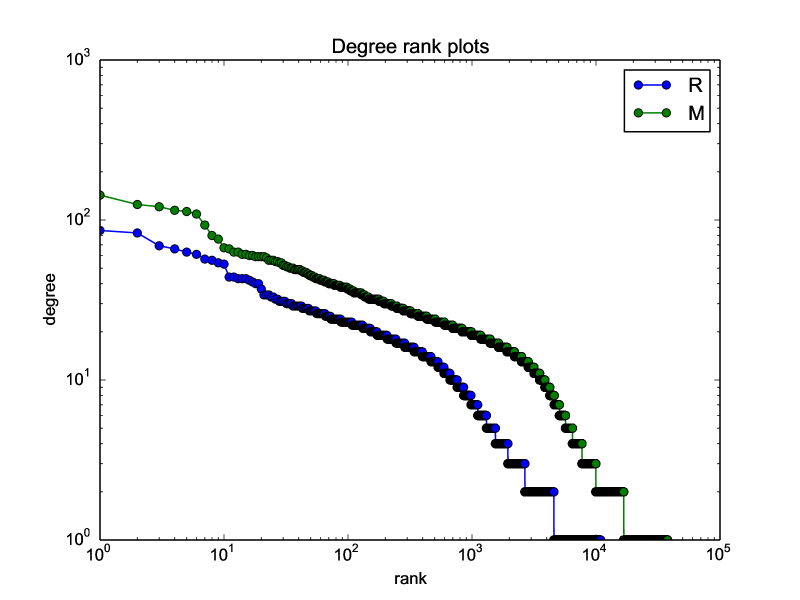
Figure 11: Degree distributions for the evolved experimental graphs

contains plots of the degree distribution in the refined graphs.

The refined graphs still contain about 65% and 72% of the original vertices for the $T_{R},T_{M}$ experiments, respectively, however, the edges are much more pruned, to about 9% and 10%, respectively. The graph density is thus lower, too (at about 20%). The numbers of connected components do not change much. This is only to be expected given the nature of the population preparation and the tendency of the evolution process to preserve connectedness. The sizes of the components are more or less proportional to the reduction of the vertex number.

What is more interesting are the component-wise characteristics of the refined graphs summarised in Table 7. The radius, diameter and average shortest path lengths are all increased by up to 78% and no less than 32%, despite of the graphs getting smaller. The clustering coefficient decreases quite radically – to about 3.8% and 5.4% of the original value for the $T_{R},T_{M}$ experiments, respectively. The vertex degree distribution still approximately follows the power law, however, the curve is not as steep as for the original graphs. These combined characteristics indicate that the refined graphs exhibit the small world property to much lower extent than the original ones. This means that they are structurally more evenly organised and tend to have less vertices or vertex groups that connect large portions of the graph through very few edges. A possible consequence of this fact is lower redundancy and higher rate of non-obvious connections in the refined graphs. Indeed, the analysis of the data w.r.t. the standard literature-based discovery application scenarios confirms this, as we show in the next section.

4.4.3 Performance of the Refined Graphs

In this section, we first discuss the performance of our experiments w.r.t. the quantitative measures used by related approaches. This is then followed by qualitative analysis of the knowledge graphs we generated.

Table 8 lists the values of the $evd$ measure for the $T_{R}$ data set. Our approach (the N column) is compared to the works [4, 42, 49, 11, 16] in columns C, S, W, G, H, respectively. For our approach, we list both $evd,evd^{r}$ values, while for the others, only $evd$ is present as they do not consider $evd^{r}$. We also provide $|G_{c}|$, i.e., the number of solution graphs with intermediates.

Intermediate	N			C [4]	S [42]	W [49]	G [11]	H [16]
	$evd$	$evd^{r}$	$|G_{c}|$
Blood Viscosity	5	0.98	1	15∗	2	Y	5	8
Platelet Aggregation	20	0.844	18	1	1	Y	6	17
Vascular Reactivity	73	0.615	4	-	1	Y	19	-

Table 8: Evidence-based evaluation – $T_{R}^{40}$ data

The $evd$ numbers correspond to the best rank of the result that contains given intermediate term. The “-” character means the intermediate cannot be found in any result for that approach. If there is “Y”, then the intermediate can be found in the results but no ranking is provided. Finally, the results with “^∗” in the C column indicate that the intermediate can only be found indirectly by manually exploring a broader context of the result [4].

Our approach finds all intermediate terms which makes its performance equivalent to or better than the related approaches in this respect. Blood viscosity and platelet aggregation are placed among the top 16% of the results (out of 205 in the $T_{R}$ experiment) while vascular reactivity is considered to be relatively less important intermediate.

Table 9 lists the same type of results as Table 8, only for the $T_{M}$ experiment and slightly different set of related works.

Intermediate	N			C [4]	S [42]	W [49]	B [2]	G [11]
	$evd$	$evd^{r}$	$|G_{c}|$
Calcium Channel
Blockers	-	-	-	22	3	Y	10	1
Epilepsy39	23	0.628	7	9∗	-	Y	8	3
Brain Anoxia /
Hypoxia	-	-	-	-	5	-	6	77
Inflammation	-	-	-	3∗	2	Y	170	82
Platelet Aggregation /
Activity10	335	0.333	2	1∗	2	Y	2	8
Prostaglandins10	352	0.274	4	4	1	Y	42	27
Serotonin	-	-	-	1	1	Y	5	1
Cortical / Spreading
Depression39	58	0.468	3	-	6	-	45	-
Vascular Mechanism /
Reactivity39	7	0.945	1	9	1	Y	46	16

Table 9: Evidence-based evaluation – $T_{M}^{39},T_{M}^{10}$ data

Note that the related works are sometimes inconsistent in the exact wording of the intermediate terms, therefore we only focused on nine out of eleven where we were able to clearly mash up the different alternatives of the term.

The quantitative results of our approach are sparser than in case of the $T_{R}$ experiment. This has been caused mainly by the minimalistic, domain-agnostic approach we chose, which resulted into relatively low coverage of the intermediate synonyms appearing in the data (the fulltext mapping could only discover terms rather similar to the canonical intermediate form used as a query, while many synonyms are quite dissimilar strings). All related approaches but one [11] use term expansion and mapping using biomedical vocabularies like MeSH, and some even use quite extensive manual interventions (see Section 5.4 for details). Despite of these limitations, we re-discovered five out of nine intermediates. Out of these, only three were discovered using a mature-enough generation of the refined knowledge graph, though.

For the intermediates we managed to find, we achieved results comparable to or better than the other approaches. For instance, three out of five related approaches were not able to re-discover the cortical depression intermediate which is considered very important in [45].

The overall results of the evidence-based evaluation are encouraging. In the $T_{R}$ experiment, our approach performed better than [4, 16], worse than [42, 11] and equally to [49]. In the $T_{M}$ experiment, we bettered [4, 49, 11] while [42, 2] outperformed us. In total, we did better than more than half of the related approaches in terms of the intermediate ranking.

The rarity and interestingness measures for the two experiments are given in Table 10.

Experiment	N		C [4]
	$rar(\mathcal{G})$	$int(\mathcal{G})$	$rar(\mathcal{G})$	$int(\mathcal{G})$
$T_{R}^{40}$	6.722	0.13	0	1
$T_{M}^{39}$	0.367	0.732	0.56	0.64

Table 10: Claim frequency-based evaluation

We can only compare ourselves to [4] as the measures were defined and used there for the first time. The average results of our approach are lower than in [4] for the $T_{R}$ experiment. However, the median rarity and interestingness of the paths generated in our experiment is 0 and 1, respectively – only about one third of the $T_{R}$ path associations have non-zero frequency on PubMed. This means that two thirds of the claims generated by our approach have the same performance in terms of rarity and interestingness as in [4]. The average results of the $T_{M}$ experiment are better in our case. More than 98% of the $T_{M}$ claims have zero rarity which clearly outperforms [4].

Before we continue with the qualitative analysis of the results, let us get back for a while to the structural properties of the refined knowledge graphs. Table 11 gives average relative ranking of the vertices corresponding to the source, target and intermediate terms in the initially extracted and refined graphs. The rankings are based on the vertex degree and betweenness centrality measures (from highest to lowest). These measures are typically used as an approximation of a vertex importance within a graph [39].

Terms	degree ranking				betw. centrality ranking
	$T_{R}^{0}$	$T_{R}^{40}$	$T_{M}^{0}$	$T_{M}^{39}$	$T_{R}^{0}$	$T_{R}^{40}$	$T_{M}^{0}$	$T_{M}^{39}$
Source, target	0.522	0.609	0.541	0.708	0.537	0.592	0.656	0.736
Intermediates	0.563	0.729	0.557	0.57	0.678	0.699	0.584	0.575

Table 11: Degree-based ranking of the re-discovery terms

The importance of sources, targets and intermediates in terms of degree is increased by the refinement in both experiments. The increase is largest for source and target terms in the $T_{M}$ experiment and for the $T_{R}$ intermediates. The importance in terms of betweenness centrality is increasing relatively less, with the $T_{M}$ intermediates actually becoming slightly less important. These observations are consistent with the evidence-based evaluation in the sense of “sensitivity” of the experimental data sets towards the source, target and intermediate terms. The refinement of the $T_{R}$ graph clearly raises the importance of all vertices, especially the intermediates. Indeed, all the terms are present in relatively highly ranking claims of the resulting $T_{R}^{40}$ graph. For the $T_{M}$ data set where only the importance of the source and target vertices is markedly rising, the results are much sparser – although the $T_{M}^{39}$ graph contains many claims connecting the source and target, there is relatively few intermediates from [45] present in these claims.

The qualitative analysis of the solution contents further elaborates on the above observations about the initial and resulting graph structure. As specified in Section 4.3.4, the analysis is based on the topics covered by the solution graphs. These are terms that provide additional context for the intermediates in the solutions. We provide comprehensive lists of the unique context topics in Appendix A, together with references to supporting literature.

The contents of the Appendix A is summarised in Table 12 which contains the $top_{d},\;top_{r},\;top_{n}$ score values for the initial and refined knowledge graphs in both experiments.

Score	$T_{R}$		$T_{M}$
	$T_{R}^{0}$	$T_{R}^{40}$	$T_{M}^{0}$	$T_{M}^{39}$
$top_{d}$	0.412	0.522	0.368	0.818
$top_{r}$	0.571	0.75	0.607	0.889
$top_{n}$	0.938	0.889	0.471	0.875

Table 12: Summary of the qualitative evaluation

The table shows that our approach improves the quality of the extracted knowledge graphs. The relative topical density $top_{r}$ (i.e., the ratio of unique topics among the paths connecting source and target terms) increases by about 27% and 122% for the $T_{R},T_{M}$ experiments, respectively. The relevance $top_{r}$ increases by about 31% and 46% for $T_{R},T_{M}$, respectively. Finally, the relative topical novelty $top_{n}$ increases by about 86% for the $T_{M}$ experiment. In case of the $T_{R}$ experiment, the measure is slightly lower for $T_{R}^{40}$ than for $T_{R}^{0}$, however, there is only one non-novel solution in both knowledge graphs. The decrease in the relative $top_{r}$ value is caused by lower total number of solutions in the refined graph.

These results confirm our assumption that the refinement improves the quality of statements extracted from literature, at least in the context of two standard literature-based discovery scenarios. The improvement in quality is three-fold. Firstly, the refined knowledge graphs are less redundant (the topical density is higher). Secondly, there is markedly more relevant solutions in the results. And thirdly, the refined solutions are largely non-obvious (high $top_{n}$ measure).

Direct and exact comparison of our qualitative results to related state of the art is unfortunately impossible due to the afore-mentioned differences in the solution representations. However, we can at least discuss the commonalities and differences informally. Figure 12 displays the hierarchy of topics covered by the $T_{R}$ results.

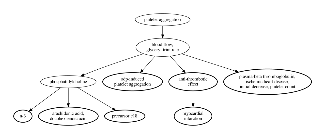
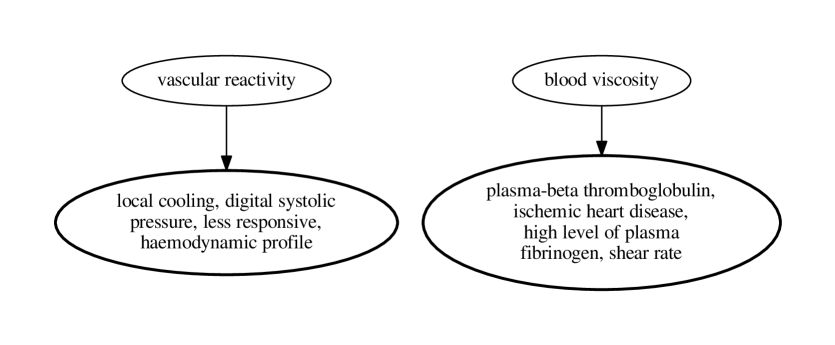
Figure 12: Hierarchy of relevant topics in $T_{R}^{40}$

Each vertex in the hierarchy graph represents a part of the topic. The roots of the presented hierarchies are the intermediate concepts. The vertices shared across multiple topics have normal outlines. Vertices that complete the topics on the way from the root have bold outlines.

The impact of glyceryl trinitrate on vasodilation and consequently also on blood flow has been studied in the context of possible treatment of Raynaud’s syndrome [19]. Our method reflects these findings in constructing a corresponding connection between Raynaud’s syndrome and platelet aggregation which is quite closely related to blood flow [17]. Phosphatidylcholine, also a relatively common vertex in the generated claims, refers to a class of phospholipids that is closely related to metabolism of fatty acids, including those found in fish oils [1]. The vertices connected to phosphatidylcholine mediate the relationship between fish oil and platelet aggregation in the solutions. The topic with ADP-induced platelet aggregation [35] specifies the type of platelet aggregation fish oils can influence. The solutions concerned with anti-thrombotic effect put this vertex in connection with fish oils, possibly with an intermediate vertex referring to myocardial infarction. This corresponds to the anti-thrombotic effect of fish oils demonstrated for instance in [52]. Finally, one of our solutions identified a link between platelet aggregation and fish oils via their influence on levels of plasma-beta thromboglobulin, a marker in ischemic heart disease [13].

The solution involving the vascular reactivity intermediate puts it in the context of influence of fish oils on lower vascular resistance, as discussed for instance in [26]. The effect of local cooling on the digital systolic pressure is inherent to Raynaud’s syndrome but its connection to the vascular reactivity discovered by our approach is more indirect. One branch of the solution involving the blood viscosity intermediate revisits the relationship between fish oils and ischemic heart disease observed in one of the claims containing platelet aggregation. The other branch is new, though, and puts the blood viscosity in relation with high levels of fibrinogen in Raynaud’s syndrome patients [46].

When comparing the contents of the $T_{R}$ solutions with related state of the art approaches, we can only refer to [4] and [44] as the other works generate mere lists of possible intermediates without further context. Many contexts associated with the intermediates as possible explanations of the connections are missing in the related works. Examples are blood flow, glyceryl trinitrate, ADP-induced platelet aggregation, phosphatidylcholine or plasma-beta thromboglobulin within ischemic heart disease. However, most of these connections are rather explanatory and not essential in the scope of Raynaud’s syndrome despite of being valid. In [4], many of the graphs involve epoprostenol (essentially a prostaglandin) as a mediator of the influence of fish oils on platelet aggregation. This is consistent with [44] that establishes the connection between fish oil and platelet aggregation as a result of increased level of prostaglandins. This context is missing in our results that involve the intermediates, however, it is present twice among the top-ten solutions (at ranks 4 and 8). Once it appears in relation to the action of the drug indomethacin, and then also in relation to luteolytic activity in women with Raynaud disease. These are potentially interesting findings that extend the results produced by comparable state of the art approaches.

Figure 13 displays the hierarchy of topics covered by the $T_{M}$ results.

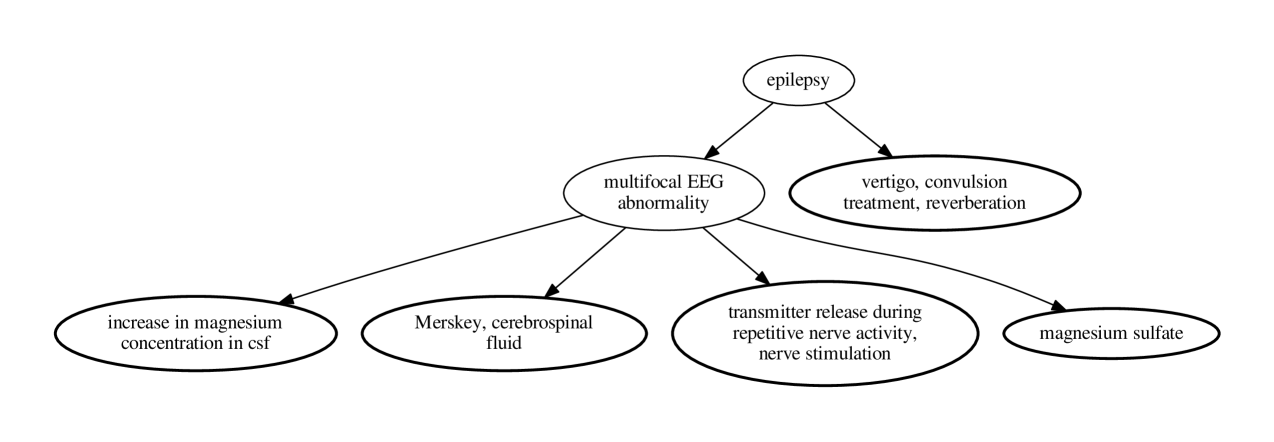
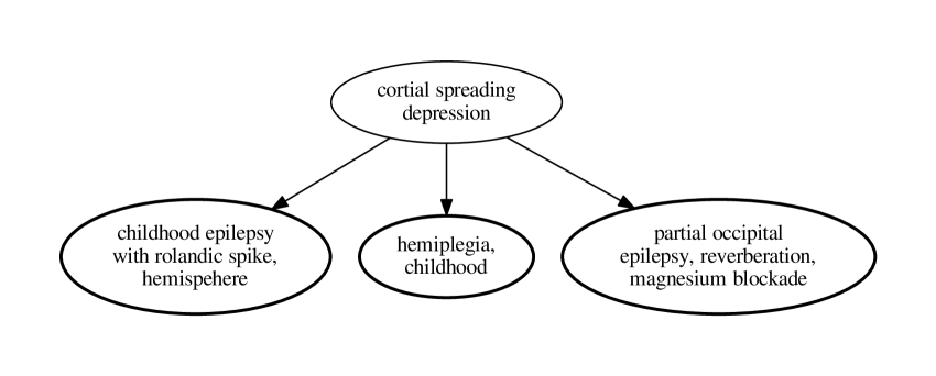
Figure 13: Hierarchy of relevant topics in $T_{M}^{39}$

One solution involving the epilepsy intermediate puts it in the context of magnesium being used as a mechanism for management of reverberating brain waves [40]. These are associated with epilepsy and vertigo attacks and the solution suggests that treatments for these conditions may be used for migraine as well. Other claims related to epilepsy all share multifocal EEG abnormalities which are characteristic for epilepsy [29]. Two different types of claims were complementing these findings – two solutions dealing with magnesium concentrations in cerebrospinal fluid in relation to migraine [37], and one solution related to transmitter release and nerve stimulation. The solutions involving the cortical spreading depression intermediate were all related to similar concepts as the epilepsy ones. This is not surprising, since cortical spreading depression is quite closely related to seizures [10].

Similarly to the $T_{R}$ experiment, we can only compare the contents of our $T_{M}$ solutions to [4] and [45] which are the only works that provide context in addition to the intermediates. The graphs presented in [4] for migraine and magnesium are generally much sparser than those for Raynaud and fish oil (typically containing only the source, target and intermediate node). Moreover, none of the results discussed in the article in detail concern epilepsy or spreading depression. The work [45] confirms close relationship between epilepsy and cortical spreading depression which is consistent with a straightforward interpretation of our results. Our solutions also managed to bring up the relationship between magnesium and cerebrospinal fluid in the context of epileptic attacks. In addition to that, our results appear to strongly associate migraine with multifocal EEG abnormalities. This is consistent with relationship between the abnormalities and headaches demonstrated for instance in [12]. Other potentially interesting findings not covered by related works are vertigo, reverberation and the relationship between migraine, cortical spreading depression and rolandic epilepsy [50].

5 Related Work

We split this section into four thematic blocks that correspond to the main theoretical and application-specific facets of our work. In particular, we review the areas of: 1. automated discovery, 2. ontology learning, 3. discovery supported by knowledge graphs, 4. literature-based discovery.

5.1 Automated Discovery

Research of ways how discoveries can be automated or facilitated by machines dates back to the dawn of the digital computer era. The work [27] provides a comprehensive analysis of the discovery process operationalised as creative problem solving. It reviews several classic machine discovery systems and the heuristics used by them, and also mentions several properties of worthy discoveries like novelty and value. A more recent related work [18] reviews the major approaches to studying the process of scientific discovery, provides another survey of automated discovery systems and analyses additional features of relevant discoveries, such as surprise. The works [21, 20] review still more machine discovery systems and heuristics, and identify features like refutability and simplicity as essential to discoveries. One of the most recent and relevant works from this area is [23]. It builds on [27, 18] and introduces formalisations of several discovery features. In particular, it models novelty and value using metric spaces, and surprise using Bayesian probabilities.

Discovery features discussed in the referenced works conform to our virtue definitions, although most of them do not provide a systematic formalisation, only rather application-specific implementations. For instance, refutability and simplicity as reviewed in [21] directly correspond to our virtues. Surprise and novelty discussed in the other works can be modelled by putting emphasis on radical claims as addressed by the conservatism virtue, only using different distance metrics for each of the respective features. We believe that our approach presents a new way to formalising discovery features that is consistent with related state of the art, but is more systematic, comprehensive and extensible. In addition, we provide an actionable set of measures implemented in the context of knowledge graphs. This enables universal applicability of our research, which is not the case in most of the rather specific afore-mentioned approaches.

5.2 Ontology Learning

In the last fifteen years, there has been a growing interest in exploring the potential of automatically extracted graph structures for knowledge discovery. Many of such approaches can be clustered under the umbrella of ontology learning [22] which aims at extracting complex statements from unstructured textual resources. This is done using specifically tailored methods from AI disciplines like natural language processing or machine learning.

As a recent survey [51] shows, the applicability of existing ontology learning approaches to (semi)automated knowledge discovery is still quite limited. Many of the techniques are dependent on manually curated resources. They also introduce a lot of assumptions during the extraction process (based on, for instance, linguistic facts valid only in the context of a particular language or discourse). This limits their universal applicability. Another problem is that the more complex knowledge representation the learned ontologies use, the more restrictive they are about their meaning. This typically leads to brittleness w.r.t. the often inherently vague and contextual nature of the knowledge they represent. This can easily cause problems in machine-aided knowledge discovery scenarios where we typically want to represent the knowledge implied by the input data in as unbiased way as possible. Another practical limitation is that most ontology learning system do not scale very well as reported in [51].

5.3 Discovery Supported by Knowledge Graphs

More recent works related to machine discovery using knowledge graphs include [6, 8, 28] which contain also comprehensive reviews of prior similar approaches. The approach elaborated in [6] presents methods for knowledge discovery in RDF [24] data based on user-defined query patterns and analytical perspectives. Our approach complements [6] by offering means for automated analysis and refinement of knowledge graphs using application-independent, well-founded features.

Google’s Knowledge Vault [8] presents a web-scale approach to probabilistic knowledge fusion that uses graphs represented in the RDF format. It tackles the scalability vs. accuracy trade-off of the manual and automatic approaches to construction of knowledge graphs. This is done by refining statements extracted from the web content using models learned from pre-existing highly accurate knowledge bases like YAGO or Freebase. Additional details and broader theoretical context of the approach introduced in [8] is given in [28], which offers a comprehensive review of relational machine learning approaches in the context of RDF-compatible knowledge graphs. The main advantage of our approach w.r.t. the works [8, 28] is that we are not critically dependent on the background knowledge model. In addition, we present a complementary well-founded approach to determining which relationships in automatically extracted knowledge graphs are worth preservation. Having said that, the techniques reviewed in [28] can certainly provide valuable hints on future extensions of our approach to graphs with oriented edges representing more than one type of relationships (i.e., RDF graphs).

5.4 Literature-Based Discovery

As our approach has been validated by experiments in literature-based discovery, we need to position ourselves within that field as well. Surveys of related works (focusing mostly on the domain of life sciences) are provided in [7, 34, 41]. The specific approaches we compare ourselves to are described in [4, 2, 16, 49, 42, 11]. In most cases where we were able to directly compare our results with the related works, our approach was at least as good as and often better than the state of the art. In addition, we managed to hint at several relevant insights that were not even discussed by the human expert in the original studies [44, 45].

The most significant advantages of our approach are, however, as follows. 1. It is absolutely automatic. The only manual action we performed was pruning the fulltext search results when mapping terms to the corresponding vertices, however, this is only required for the evaluation, not for the method itself. 2. There are no domain-specific dependencies and thus our work is readily applicable to any field, not just the biomedical literature-based discovery. 3. We produce extensive contextual information that can facilitate the interpretation of the results and thus make the machine-aided discovery process more efficient. 4. Our approach is based on theoretical foundations motivated by the state of the art philosophical study of key features of scientific discoveries.

The works [42, 16, 49] all depend on rather extensive manual effort (definition of semantic types and discovery patterns, result pruning, etc.). The approaches [4, 2, 11] are automated, however, only [4] provides broader context in order to elucidate the connections. Moreover, all works but [11] substantially rely on an external domain-specific source of background knowledge and/or domain-specific NLP tools, namely the MeSH and UMLS vocabularies [3] and the tools SemRep [38] and BioMedLEE [5]. It is quite plausible to assume that without these resources, the related approaches dependent on them would perform much less favourably when compared to our implementation. Last but not least, all the related approaches lack the universally applicable theoretical foundations presented as the core contribution of this article.

6 Conclusions and Future Work

We have presented a novel approach to discovery informatics that is based on formalisation of hypothesis virtues in the context of knowledge graphs. We have shown that the approach is naturally motivated, well-founded, extensible and universally applicable. It can be used as a broader theoretical frame for other approaches to machine discovery, as briefly outlined in Section 5. We have delivered an implementation of the presented research and performed its experimental validation using standard scenarios in literature-based discovery. A successful comparison with related state of the art tools demonstrates the practical relevance of our work.

In near future, we will extend the theoretical framework in order to address directed multi-graphs with predicate edge labels and more complex semantics associated with particular edge and vertex types. This will allow for straightforward application of our approach to more expressive knowledge graphs, such as RDF [24] knowledge bases and ontologies in the Linked Open Data cloud [14]. Furthermore, we intend to continue demonstrating the universality of our framework by using it in other experimental scenarios targeted by related works in machine discovery. We also plan to explore the complex relationships between specific measures and their influence on the properties of the evolutionary refinement process (e.g., convergence, optimality and completeness bounds). This will lead to deeper understanding of the refinement, and therefore also to more efficient implementations. Finally, and perhaps most importantly, we would like to use our approach in scenarios involving actual new discoveries, in direct collaboration with corresponding domain experts.

References

Appendix A: Context Topics for the Intermediate Terms

This appendix presents tables with the context topics of the intermediate terms for the initial and refined graphs in the $T_{R},T_{M}$ experiments. Each table contains topics for one intermediate within a specific experimental graph. The topics are given in the first column. The second column of each table states whether or not the corresponding topics are relevant. Topics with relevant part subsumed by another relevant topic are not considered relevant unless they extend the subsumed part with new relevant information. If there is an exclamation mark in the second column (applicable only to relevant topics), it means the relationship expressed by the corresponding solution is novel, i.e., not covered in any single existing article published by March, 2015. The third column lists references of articles that jointly provide support of relevant claims. We use easily de-referencable PubMed identifiers for brevity. Note that more common and/or simple relationships may have alternative sets of supporting articles that do not appear in the lists provided here.

First we provide three tables for the initial graph $T_{R}^{0}$ in the $T_{R}$ experiment (Table 13-15) and three tables for the refined graph $T_{R}^{40}$ (Table 16-18).

Topics	Rel.	Support
glyceril trinitrate, blood flow, myocardial infarction	Y!	17311994, 14831190, 10604966, 3092847, 9310278
glyceril trinitrate, blood flow, precursor c18, c20	N	N/A
glyceril trinitrate, blood flow, phosphatidylcholine, arachidonic acid	Y!	17311994, 9675609, 4205973, 14831190, 10604966, 3092847
glyceril trinitrate, blood flow, aa and docosahexaenoic acid	N	N/A
glyceril trinitrate, blood flow, phosphatidylcholine, individual phospholipid, alteration and recovery	N	N/A
glyceril trinitrate, blood flow, antithrombin iii	Y!	17311994, 18370504, 14831190, 10604966, 3092847
glyceril trinitrate, blood flow, adp-induced platelet aggregation	Y!	17311994, 10086317, 18370504, 14831190, 10604966, 3092847
glyceril trinitrate, blood flow, adp-induced platelet aggregation, corn oil	N	N/A
glyceril trinitrate, blood flow, linseed	N	N/A
glyceril trinitrate, blood flow, thrombin and collagen	Y!	17311994, 4468230, 18370504, 14831190, 10604966, 3092847
glyceril trinitrate, blood flow, collagen, precursor c18	N	N/A
glyceril trinitrate, blood flow, adp-induced platelet aggregation, vasospastic disease, prostaglandin e1	Y!	17311994. 10086317, 18370504, 14831190, 10604966, 3092847
glyceril trinitrate, blood flow, low pufa coconut oil adp–induced platelet aggregation	N	N/A
alpha-adrenergic receptor	N	N/A
prostacyclin, thromboxane, adp-induced platelet aggregation	Y!	10086317, 6258879, 19037602
upper limb, arteritis, haemodynamic profile	N	N/A
alpha-adrenergic receptor, adp-induced platelet aggregation	Y	34707

Table 13: Topic contexts for platelet aggregation in $T_{R}^{0}$

Topics	Rel.	Support
glyceryl trinitrate, blood flow, hand, cold	N	N/A
glyceryl trinitrate, blood flow, hand, cold, myocardial infarction	Y!	24753696, 9310278, 10086317, 18370504, 14831190
vascular dilation, cold, myocardial infarction	Y!	9310278, 15695304
upper limb, arteritis, haemodynamic profile, myocardial infarction	N	N/A
local cooling, digital systolic pressure, haemodynamic profile, less responsive, myocardial infarction	Y!	9310278, 22453196, 17876193
cold spell, radiological investigation	N	N/A

Table 14: Topic contexts for vascular reactivity in $T_{R}^{0}$

Topics	Rel.	Support
finger systolic pressure, dazoxiben treatment, high level of plasma fibrinogen	Y!	6393521, 7459607
fibrinolytic enhancement, high level of plasma fibrinogen	Y!	698554, 7459607
fibrinolytic enhancement, deformability index	Y!	698554, 519354
finger systolic pressure, dazoxiben treatment, high level of plasma fibrinogen, shear rate	Y!	6393521, 7459607, 579511
finger systolic pressure, dazoxiben treatment, high level of plasma fibrinogen, shear rate, fibrinolytic enhancement, deformability index	Y!	6393521, 7459607, 579511, 519354

Table 15: Topic contexts for blood viscosity in $T_{R}^{0}$

Topics	Rel.	Support
n-3, phosphatidylcholine, blood flow, glyceryl trinitrate	Y!	17311994, 9675609, 24679762, 14831190, 10604966, 3092847
phosphatidylcholine, aa and docohexaenoic acid, arachidonic acid, blood flow, glyceryl trinitrate	Y!	17311994, 9675609, 4205973, 14831190, 10604966, 3092847
plasma-beta-thromboglobulin, ischemic heart disease, platelet count, initial decrease, blood flow, glyceryl trinitrate	Y!	17311994, 6123019, 14831190, 10604966, 3092847
adp-induced platelet aggregation, blood flow, glyceryl trinitrate	Y!	17311994, 10086317, 18370504, 14831190, 10604966, 3092847
anti-thrombotic effect, blood flow, glyceryl trinitrate	Y!	17311994, 6294902, 14831190, 10604966, 3092847
anti-thrombotic effect, myocardial infarction, blood flow, glyceryl trinitrate	Y!	17311994, 6294902, 9310278, 14831190, 10604966, 3092847
n-3, phosphatidylcholine, blood flow, glyceryl trinitrate, alteration and recovery	N	N/A
n-3, phosphatidylcholine, blood flow, glyceryl trinitrate, alteration and recovery, individual phospholipid	N	N/A
precursor c18, phosphatidylcholine, blood flow, glyceryl trinitrate	Y!	17311994, 9675609, 4205973, 14831190, 10604966, 3092847

Table 16: Topic contexts for platelet aggregation in $T_{R}^{40}$

Topics	Rel.	Support
local cooling, digital systolic pressure, less responsive, haemodynamic profile	Y	22453196, 17876193
upper limb, arteritis, haemodynamic profile, myocardial infarction	N	N/A

Table 17: Topic contexts for vascular reactivity in $T_{R}^{40}$

Topics	Rel.	Support
plasma-beta-thromboglobulin, ischemic heart disease, high level of plasma fibrinogen, shear rate	Y!	6123019, 579511, 519354

Table 18: Topic contexts for blood viscosity in $T_{R}^{40}$

The topics for the $T_{M}$ experiment are organised in five tables for the initial graph $T_{M}^{0}$ (Table 19-23) and in three tables for the refined graph $T_{M}^{39}$ (Table 24-26).

Topics	Rel.	Support
acute intrapartum fetal distress	N	N/A
flunarizine, seizure	Y	25754865, 3332609, 22406257
toxemia, horton	Y!	25754865, 25373431, 14401618, 6557975
bulbo-cortical pathway	Y	25754865, 3609865
sea water	N	N/A
m.e.p.p., inhibitory effect of prostaglandin on vasopressin	N	N/A
brachymetapody, inhibitory effect of prostaglandin on vasopressin, cyanosis	N	N/A
fibrinolysis, lipid, vascular disease	Y!	25754865, 20669129, 25737193
antiserotonin, toxemia	Y!	25754865, 25373431, 5315778
spasmophilia, magnesium sulfate	Y	25754865, 9340190
cyanosis, limb, inhibitory effect of prostaglandin on vasopresin, magnesium excretion	N	N/A
conventional therapy for vertigo	Y	25754865, 23837033
amonium	Y	25754865, 10897167
verapamil, magnesium blockade	Y!	25754865, 23973639, 24113539, 8891316
increase in bathing, washing	Y!	25754865, 2294020025667882
ketonic body	Y	25754865, 24300035
merskey, cerebrospinal fluid	Y	25754865, 6100318

Table 19: Topic contexts for epilepsy in $T_{M}^{0}$

Topics	Rel.	Support
alkaline phosphatase, hydroxyproline	N	N/A
magnesium chloride	Y!	25238714, 25010639, 24828386,
immunoreactive, hyposmotic stress	N	N/A

Table 20: Topic contexts for prostaglandin in $T_{M}^{0}$

Topics	Rel.	Support
magnesium blockade, benign syndrome	N	N/A

Table 21: Topic contexts for cortical spreading depression in $T_{M}^{0}$

Topics	Rel.	Support
indomethacin	Y	22529203, 2925371
high calcium	Y!	12010379, 2925371, 15152357

Table 22: Topic contexts for vascular reactivity in $T_{M}^{0}$

Topics	Rel.	Support
fatty acid level, aspirin, dipyridamole, epilepsy	Y!	25741817, 25116182, 10775263, 22749692
cholesterol	N	N/A
endocarditis, vasculomotor reaction, epilepsy	Y!	3513926, 21762000
prostaglandin synthesis, potent anti-inflammatory agent	N	N/A

Table 23: Topic contexts for platelet aggregation in $T_{M}^{0}$

Topics	Rel.	Support
transmitter release during repetitive nerve activity, nerve stimulation, multifocal EEG abnormality	Y!	25754865, 2446959, 13175198
multifocal EEG abnormality, magnesium sulfate	Y!	25754865, 2446959, 23256267
vertigo, convulsion treatment, reverberation	Y!	25754865, 23837033
multifocal EEG abnormality, merskey, cerebrospinal fluid	Y!	25754865, 2446959, 6100318
multifocal EEG abnormality, plasma, increase in magnesium concentration in csf	Y!	25754865, 2446959, 3981211

Table 24: Topic contexts for epilepsy in $T_{M}^{39}$

Topics	Rel.	Support
childhood epilepsy with rolandic spike, hemisphere	Y!	25754865, 19271946, 19674062, 22961355
hemiplegia, childhood	Y	25754865, 23907418, 21490217
partial occipital epilepsy, reverberation, magnesium blockade	Y!	25754865, 23907418, 1283483, 1110377

Table 25: Topic contexts for cortical spreading depression in $T_{M}^{39}$

Topics	Rel.	Support
high calcium, tension headache	N	N/A

Table 26: Topic contexts for vascular reactivity in $T_{M}^{39}$

References

- Abe et al. [2014] Abe, E., Ikeda, K., Nutahara, E., Hayashi, M., Yamashita, A., Taguchi, R., Doi, K., Honda, D., Okino, N., Ito, M., 2014. Novel lysophospholipid acyltransferase PLAT1 of aurantiochytrium limacinum F26-b responsible for generation of palmitate-docosahexaenoate-phosphatidylcholine and phosphatidylethanolamine. PloS one 9 (8), e102377.
- Blake and Pratt [2002] Blake, C., Pratt, W., 2002. Automatically identifying candidate treatments from existing medical literature. In: AAAI Spring Symposium on Mining Answers from Texts and Knowledge Bases. pp. 9–13.
- Bodenreider [2004] Bodenreider, O., 2004. The unified medical language system (UMLS): integrating biomedical terminology. Nucleic acids research 32 (suppl 1), D267–D270.
- Cameron et al. [2015] Cameron, D., Kavuluru, R., Rindflesch, T. C., Sheth, A. P., Thirunarayan, K., Bodenreider, O., 2015. Context-driven automatic subgraph creation for literature-based discovery. Journal of Biomedical Informatics. In press.
- Chen and Friedman [2004] Chen, L., Friedman, C., 2004. Extracting phenotypic information from the literature via natural language processing. Medinfo 11 (Pt 2), 758–62.
- Colazzo et al. [2014] Colazzo, D., Goasdoué, F., Manolescu, I., Roatis, A., 2014. RDF Analytics: Lenses over Semantic Graphs. In: Proceedings of WWW’14. ACM.
- de Bruijn and Martin [2002] de Bruijn, B., Martin, J., 2002. Getting to the (c)ore of knowledge: mining biomedical literature. International Journal of Medical Informatics 67 (1–3), 7 – 18.
- Dong et al. [2014] Dong, X., Gabrilovich, E., Heitz, G., Horn, W., Lao, N., Murphy, K., Strohmann, T., Sun, S., Zhang, W., 2014. Knowledge vault: A web-scale approach to probabilistic knowledge fusion. In: Proceedings of the 20th ACM SIGKDD international conference on Knowledge discovery and data mining. ACM, pp. 601–610.
- Eiben and Smith [2007] Eiben, A. E., Smith, J., 2007. Introduction to Evolutionary Computing. Springer.
- Fabricius et al. [2008] Fabricius, M., Fuhr, S., Willumsen, L., Dreier, J. P., Bhatia, R., Boutelle, M. G., Hartings, J. A., Bullock, R., Strong, A. J., Lauritzen, M., 2008. Association of seizures with cortical spreading depression and peri-infarct depolarisations in the acutely injured human brain. Clinical Neurophysiology 119 (9), 1973–1984.
- Gordon and Lindsay [1996] Gordon, M. D., Lindsay, R. K., 1996. Toward discovery support systems: A replication, re-examination, and extension of Swanson’s work on literature-based discovery of a connection between Raynaud’s and fish oil. Journal of the American Society for Information Science 47 (2), 116–128.
- Guidetti et al. [1986] Guidetti, V., Fornara, R., Marchini, R., Moschetta, A., Pagliarini, M., Ottaviano, S., Seri, S., 1986. Headache and epilepsy in childhood: analysis of a series of 620 children. Functional neurology 2 (3), 323–341.
- Hay et al. [1982] Hay, C., Durber, A., Saynor, R., 1982. Effect of fish oil on platelet kinetics in patients with ischaemic heart disease. The Lancet 319 (8284), 1269–1272.
- Heath and Bizer [2011] Heath, T., Bizer, C., 2011. Linked Data: Evolving the Web Into a Global Data Space. Morgan & Claypool.
- Honavar [2014] Honavar, V. G., 2014. The promise and potential of big data: A case for discovery informatics. Review of Policy Research 31 (4), 326–330.
- Hristovski et al. [2006] Hristovski, D., Friedman, C., Rindflesch, T. C., Peterlin, B., 2006. Exploiting semantic relations for literature-based discovery. In: AMIA annual symposium proceedings. Vol. 2006. American Medical Informatics Association, p. 349.
- Jackson [2007] Jackson, S. P., 2007. The growing complexity of platelet aggregation. Blood 109 (12), 5087–5095.
- Klahr and Simon [1999] Klahr, D., Simon, H. A., 1999. Studies of scientific discovery: Complementary approaches and convergent findings. Psychological Bulletin 125 (5), 524.
- Kleckner et al. [1951] Kleckner, M. S., Allen, E. V., Wakim, K. G., 1951. The effect of local application of glyceryl trinitrate (nitroglycerine) on Raynaud’s disease and Raynaud’s phenomenon studies on blood flow and clinical manifestations. Circulation 3 (5), 681–689.
- Langley [2000] Langley, P., 2000. The computational support of scientific discovery. International Journal of Human-Computer Studies 53 (3), 393 – 410.
- Langley and Zytkow [1989] Langley, P., Zytkow, J. M., 1989. Data-driven approaches to empirical discovery. Artificial Intelligence 40 (1-3), 283–312.
- Maedche and Staab [2004] Maedche, A., Staab, S., 2004. Ontology learning. In: Staab, S., Studer, R. (Eds.), Handbook on Ontologies. Springer, Ch. 9, pp. 173–190.
- Maher and Fisher [2012] Maher, M. L., Fisher, D. H., 2012. Using AI to evaluate creative designs. In: 2nd International Conference on Design Creativity, Glasgow, UK.
- Manola and Miller [2004] Manola, F., Miller, E., 2004. RDF Primer. Available at (November 2008): http://www.w3.org/TR/rdf-primer/.
- Mowshowitz and Dehmer [2012] Mowshowitz, A., Dehmer, M., 2012. Entropy and the complexity of graphs revisited. Entropy 14 (3), 559–570.
- Mozaffarian [2007] Mozaffarian, D., 2007. Fish, n-3 fatty acids, and cardiovascular haemodynamics. Journal of Cardiovascular Medicine 8, S23–S26.
- Newell et al. [1959] Newell, A., Shaw, J. C., Simon, H. A., 1959. The processes of creative thinking. Rand Corporation Santa Monica, CA.
- Nickel et al. [2015] Nickel, M., Murphy, K., Tresp, V., Gabrilovich, E., 2015. A review of relational machine learning for knowledge graphs: From multi-relational link prediction to automated knowledge graph construction. arXiv preprint arXiv:1503.00759.
- Noriega-Sanchez and Markand [1976] Noriega-Sanchez, A., Markand, O. N., 1976. Clinical and electroencephalographic correlation of independent multifocal spike discharges. Neurology 26 (7), 667–667.
- Nováček and Burns [2014] Nováček, V., Burns, G. A., 2014. SKIMMR: Facilitating knowledge discovery in life sciences by machine-aided skim reading. PeerJ. Available at https://peerj.com/articles/483/.
- Onnela et al. [2007] Onnela, J.-P., Saramäki, J., Hyvönen, J., Szabó, G., Lazer, D., Kaski, K., Kertész, J., Barabási, A.-L., 2007. Structure and tie strengths in mobile communication networks. Proceedings of the National Academy of Sciences 104 (18), 7332–7336.
- Pedregosa et al. [2011] Pedregosa, F., Varoquaux, G., Gramfort, A., Michel, V., Thirion, B., Grisel, O., Blondel, M., Prettenhofer, P., Weiss, R., Dubourg, V., Vanderplas, J., Passos, A., Cournapeau, D., Brucher, M., Perrot, M., Duchesnay, E., 2011. Scikit-learn: Machine learning in Python. Journal of Machine Learning Research 12, 2825–2830.
- Popper [2005] Popper, K., 2005. The logic of scientific discovery. Routledge.
- Preiss et al. [2012] Preiss, J., Stevenson, M., McClure, M. H., 2012. Towards semantic literature based discovery. In: 2012 AAAI Fall Symposium Series: Information Retrieval and Knowledge Discovery in Biomedical Text. Vol. 30. AAAI, pp. 7–18.
- Puri [1999] Puri, R. N., 1999. ADP-induced platelet aggregation and inhibition of adenylyl cyclase activity stimulated by prostaglandins: signal transduction mechanisms. Biochemical pharmacology 57 (8), 851–859.
- Quine and Ullian [1978] Quine, W. V., Ullian, J. S., 1978. The Web of Belief. McGraw-Hill.
- Ramadan et al. [1989] Ramadan, N., Halvorson, H., Vande-Linde, A., Levine, S. R., Helpern, J., Welch, K., 1989. Low brain magnesium in migraine. Headache: The Journal of Head and Face Pain 29 (9), 590–593.
- Rindflesch et al. [2005] Rindflesch, T. C., Fiszman, M., Libbus, B., 2005. Semantic interpretation for the biomedical research literature. In: Medical informatics. Springer, pp. 399–422.
- Scott [2012] Scott, J., 2012. Social network analysis. Sage.
- Shibata and Bures [1975] Shibata, M., Bures, J., 1975. Techniques for termination of reverberating spreading depression in rats. Journal of neurophysiology 38 (1), 158–166.
- Smalheiser [2012] Smalheiser, N. R., 2012. Literature-based discovery: Beyond the ABCs. Journal of the American Society for Information Science and Technology 63 (2), 218–224.
- Srinivasan [2004] Srinivasan, P., 2004. Text mining: generating hypotheses from MEDLINE. Journal of the American Society for Information Science and Technology 55 (5), 396–413.
- Stegmann and Grohmann [2003] Stegmann, J., Grohmann, G., 2003. Hypothesis generation guided by co-word clustering. Scientometrics 56 (1), 111–135.
- Swanson [1986] Swanson, D. R., 1986. Fish oil, Raynaud’s syndrome, and undiscovered public knowledge. Perspectives in Biology and Medicine 30 (1), 7–18.
- Swanson [1987] Swanson, D. R., 1987. Migraine and magnesium: eleven neglected connections. Perspectives in Biology and Medicine 31 (4), 526–557.
- Tietjen et al. [1975] Tietjen, G. W., Chien, S., Leroy, E. C., Gavras, I., Gavras, H., Gump, F. E., 1975. Blood viscosity, plasma proteins, and Raynaud syndrome. Archives of Surgery 110 (11), 1343–1346.
- Valiant [1979] Valiant, L. G., 1979. The complexity of enumeration and reliability problems. SIAM Journal on Computing 8 (3), 410–421.
- Watts and Strogatz [1998] Watts, D. J., Strogatz, S. H., 1998. Collective dynamics of ’small-world’ networks. Nature 393 (6684).
- Weeber et al. [2001] Weeber, M., Klein, H., de Jong-van den Berg, L., Vos, R., et al., 2001. Using concepts in literature-based discovery: Simulating swanson’s Raynaud–fish oil and migraine–magnesium discoveries. Journal of the American Society for Information Science and Technology 52 (7), 548–557.
- Wirrell and Hamiwka [2006] Wirrell, E. C., Hamiwka, L. D., 2006. Do children with benign rolandic epilepsy have a higher prevalence of migraine than those with other partial epilepsies or nonepilepsy controls? Epilepsia 47 (10), 1674–1681.
- Wong et al. [2012] Wong, W., Liu, W., Bennamoun, M., 2012. Ontology learning from text: A look back and into the future. ACM Comput. Surv. 44 (4), 20:1–20:36.
- Zhu and Parmley [1990] Zhu, B.-Q., Parmley, W. W., 1990. Modification of experimental and clinical atherosclerosis by dietary fish oil. American heart journal 119 (1), 168–178.