Agreement of classical Kubo theory
with the infrared dispersion curves $n(\omega)$ of ionic crystals

Abstract

The theoretical dispersion curves $n(\omega)$ (refractive index versus frequency) of ionic crystals in the infrared domain are expressed, within the Green–Kubo theory, in terms of a time correlation function involving the motion of the ions only. The aim of this paper is to investigate how well the experimental data are reproduced by a classical approximation of the theory, in which the time correlation functions are expressed in terms of the ions orbits. We report the results of molecular dynamics (MD) simulations for the ions motions of a LiF lattice of 4096 ions at room temperature. The theoretical curves thus obtained are in surprisingly good agreement with the experimental data, essentially over the whole infrared domain. This shows that at room temperature the motion of the ions develops essentially in a classical regime.

PACS: 63.20.dk, 63.20.Ry, 78.20.Ci

Experimental data on the dispersion curves $n(\omega)$ – refractive index versus angular frequency – of ionic crystals in the infrared domain have been available for a long time [1]. However, a microscopic explanation covering the whole infrared domain is apparently lacking, notwithstanding the fact that the general theoretical frame is well defined. On the other hand, a recent work [2] (see also [3]) has shown that the dispersion relation $\omega(\mathbf{k})$ in ferroelectrics can be calculated through MD simulations. In this paper we show that a calculation of the ions motions through MD simulations leads to theoretical dispersion curves $n(\omega)$ for ionic crystals which agree in a surprisingly good way with the experimental data essentially over the whole infrared domain. In fact, the problem can be dealt with through MD simulations because by Green–Kubo theory the refractive index is expressed in terms of a time correlation function involving the microscopic dipole moment $\mathbf{P}$ due to the ions motions.

Let us recall the theoretical frame. The refractive index is just the square root of the electric permittivity tensor ${\varepsilon}={\varepsilon}_{ij}(\omega)$, which in turn is related to the dielectric susceptibility tensor $\chi(\omega)$ through

$${\varepsilon}_{ij}(\omega)=\delta_{ij}+4\pi\chi_{ij}(\omega)\ .$$ (1)

Now, the susceptibility tensor $\chi(\omega)$ is the response function of the considered medium to an external electric field, so that the Green-Kubo theory provides for it a formula involving a microscopic quantity, the polarization $\mathbf{P}(t)$. For a ionic crystal the contribution to polarization in the infrared range comes mainly from the ions. So the microscopic polarization can be written as

$$\mathbf{P}=\frac{1}{V}\sum_{\mathbf{h},s}e_{s}\mathbf{q}_{s,\mathbf{h}}\ ,$$ (2)

where $\mathbf{q}_{s,\mathbf{h}}$ is the displacement of the ion of the $s$ species (having charge $e_{s}$) in the $\mathbf{h}$–th cell from its equilibrium position, and the summation is understood over all ions belonging to the (small) volume $V$.

The quantum theoretical formula for the ionic contribution to susceptibility is given for instance in [4] (see formula (2.16a)) and in [5]. For a review see [6]. The corresponding classical limit is then (see formula (2.16b) in [4], or see [7] for a purely classical deduction)

$$\chi_{ij}(\omega)=\beta V\int_{0}^{+\infty}e^{-i\omega t}\langle P_{i}(t)\dot{P}_{j}(0)\rangle dt\ .$$ (3)

Here, as usual, $\beta=1/k_{B}T$ is inverse temperature with $k_{B}$ the Boltzmann constant, while $\langle\ldots\rangle$ denotes ensemble average.

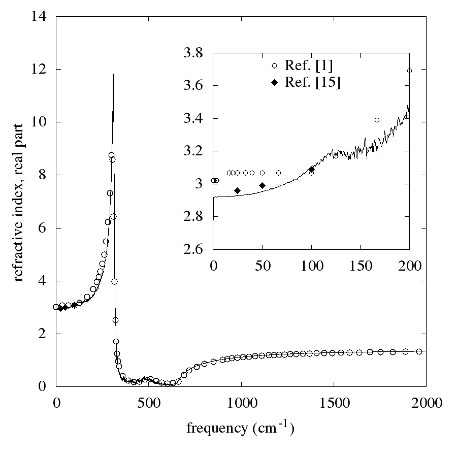
Figure 1: Real part of the refractive index versus frequency for a LiF crystal at 300 K. Circles and diamonds are experimental data taken from [1] and [15] respectively. Solid line is obtained, through Green–Kubo theory, from MD simulations for the motions of a system of 4096 ions. The inset is a zoom of the leftmost part of the figure.

Instead, the contribution of the electrons to susceptibility in the infrared is well known from experiments to just reduce to a constant (isotropic) tensor $\chi^{(\infty)}\delta_{ij}$, which can be taken from [1].

Thus the computation of the refractive index in the infrared range is reduced to a computation of the ionic susceptibility, which in turn is reduced, through (3) and (2), to a determination of the classical motions of the ions.

So, we model the crystal as a face centered cubic lattice of $2N$ particles (the ions, with their atomic masses) in a cubic box of side $L=l_{0}(N/4)^{\frac{1}{3}}$, where $l_{0}$ is the lattice constant. The ions interact through mutual electric forces, and through a phenomenological short–range repulsive pair potential $V_{rep}$. Periodic boundary conditions are imposed, and the equilibrium positions $\mathbf{x}_{s,\mathbf{h}}$ of the atomic species $s=1,2$ in the cell $\mathbf{h}\in\mathbb{Z}^{3}$ of the lattice, as well as the value of the lattice constant $l_{0}$, are taken from the literature [8]. In the numerical simulations, we took $2N=4096$.

For the aim of estimating the electric forces between ions, it is known (see [9]) that the ions can be dealt with as point particles only if a suitable “effective charge” $e_{eff}$ is substituted for the ions charge. In this paper we concentrate on lithium fluoride, which is the halide presenting the simplest infrared spectrum, using for it the value given in the literature (see [10]), namely $e_{eff}=0.81e$, where $e$ is the electron charge.

Concerning the phenomenological repulsive short–range pair potential $V_{rep}$, in the literature one often takes it to be spherically symmetric, independent of the ions’ species, and depending on the distance $r$ as an exponential, $a\exp(-r/r^{*})$. Here we chose the analytic form previously considered by Born in his MIT lectures [11] and in the paper [12], namely, $V_{rep}(r)=a\,r^{-p}$, with a cut–off at 5 Å. Thus, having fixed the effective charge, the model still contains two free parameters, $a$ and $p$. We are confident that the choice of the repulsive potential, exponential or inverse power, doesn’t play an essential role.

The two parameters $a$ and $p$ can in principle be determined through the thermodynamic available data, for example from the compressibility and the heat of formation. Here we determined them from the experimental dispersion relation $\omega(\mathbf{k})$ obtained from neutron scattering. To this end we made reference to the work [12], which was devoted to an analytical estimate of the dispersion relation in the linear approximation with the aim of a microscopic explanation of the existence of polaritons. In that work the elastic constants of the crystal had to be determined by fit with the experimental curves. As the elastic constants are related to the first two derivatives of the phenomenological potential $V_{rep}$ (see [13]), this information, together with the choice that $p$ be an integer, allowed to determine $a=1.25$ and $p=6$.

Figure 2: Imaginary part of the refractive index versus frequency for a LiF crystal at 300 K. As in figure 1, circles are experimental data taken from [1], while solid line is obtained, through Green–Kubo theory, from MD simulations for the motions of a system of 4096 ions.

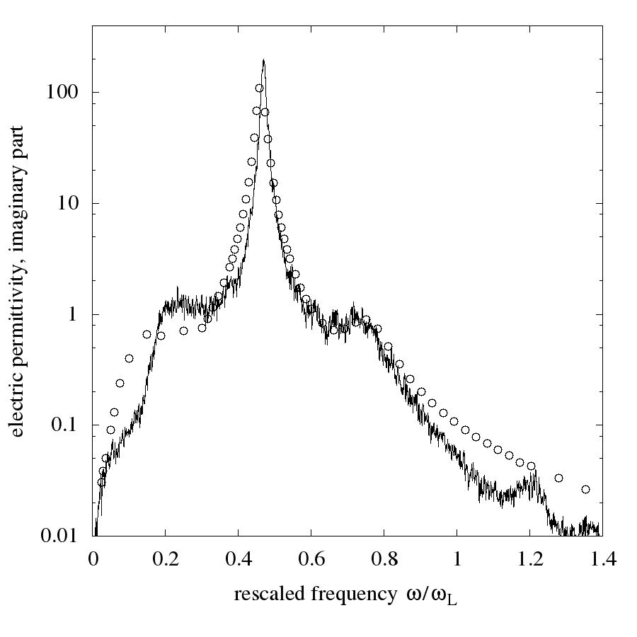
Figure 3: Imaginary part of the electric permittivity ${\varepsilon}$ (in logarithmic scale) versus rescaled frequency $X=\omega/\omega_{L}$, where $\omega_{L}=665$ cm^-1 is the frequency of the zero longitudinal optical mode. Circles are experimental data from [1], while solid line is obtained, through Green–Kubo theory, from MD simulations for the motions of a system of 4096 ions. Compare with the theoretical curve reported in Fig. 12 of ref. [21], obtained with quantum mechanical methods. Note that the experimental data reported there are the older ones [22] and [23]. The agreement with the new data [1] reported here is apparently better.

Concerning the electric forces, due to their long–range nature a problem arises in writing down explicitly the equations of motion when periodic boundary conditions are imposed, because one then has to determine the electric field produced by an infinite lattice of charges. As is well known (see [14]), the problem is solved in a computationally efficient way using the Ewald resummation formula. This amounts to introducing the potential

$$\begin{split}V_{Coul}=\sum_{s,\mathbf{h}}\sum_{s^{\prime},\mathbf{h}^{\prime}}(-1)^{s+s^{\prime}}e^{2}_{eff}\left[\sideset{}{{}^{\prime}}{\sum}_{\mathbf{n}\in\mathbb{Z}^{3}}\frac{\mathrm{erfc}(\delta|\mathbf{r}^{(s,s^{\prime})}_{\mathbf{h},\mathbf{h}^{\prime}}+\mathbf{n}\,L|)}{|\mathbf{r}^{(s,s^{\prime})}_{\mathbf{h},\mathbf{h}^{\prime}}+\mathbf{n}\,L|}\right.\\ +\left.\frac{4\pi}{L^{3}}\sum_{\mathbf{k}\in\mathbb{Z}^{3}}\exp\left(-\frac{\pi^{2}|\mathbf{k}|^{2}}{\delta^{2}L^{2}}\right)\exp\left(i\frac{2\pi}{L}\mathbf{k}\cdot\mathbf{r}^{(s,s^{\prime})}_{\mathbf{h},\mathbf{h}^{\prime}}\right)\right]\end{split}$$

where $\mathrm{erfc}(x)$ is the complementary error function, $\delta$ is a parameter to be chosen to insure fast convergences of the series, $\mathbf{r}^{(s,s^{\prime})}_{\mathbf{h},\mathbf{h}^{\prime}}=(\mathbf{x}_{s,\mathbf{h}}+\mathbf{q}_{s,\mathbf{h}})-(\mathbf{x}_{s^{\prime},\mathbf{h}^{\prime}}+\mathbf{q}_{s^{\prime},\mathbf{h}^{\prime}})$ and the primed sum over $\mathbf{n}$ means that the term for $\mathbf{n}=0$ is omitted if $s=s^{\prime}$ and $\mathbf{h}=\mathbf{h}^{\prime}$. We took $\delta=0.2$ Å^-1 which allows to truncate the series at $|n_{x}|,|n_{y}|,|n_{z}|\leq N_{max}=1$ and $|k_{x}|,|k_{y}|,|k_{z}|\leq K_{max}=3$.

The numerical integrations of the equations of motion were performed with a standard symplectic Verlet method. The integration step was taken equal to $2$ fs, the duration of each simulation was of 100 ps, and the time averages (which will be mentioned in a moment) were taken over 50 ps. The initial data for each orbit were assigned by setting the particles in their equilibrium positions, while the velocities were extracted according to the Maxwell–Boltzmann distribution, with the constraint that the center of mass of the system has vanishing velocity. Then, the temperature of the system (300 K) was determined through the mean kinetic energy, once thermalization had been attained.

So we computed the orbits, i.e. the displacement $\mathbf{q}_{s,\mathbf{h}}(t)$ of the ions from their equilibrium positions, for a LiF lattice of 4096 ions at 300 K, and thus the microscopic polarization $\mathbf{P}(t)$ too, given by (2). In formula (3) for the susceptibility the ensemble average was estimated as the mean value, over 10 different orbits, of the corresponding time average.

As a check for our computations we controlled that the susceptibility tensor actually is, as expected for LiF, an isotropic one. Namely, the off–diagonal matrix elements are negligible and the diagonal ones can be considered as equal. One may presume that these properties should not occur in a less symmetric type of crystal, so that phenomena of optical activity would show up in such cases. In our case, however, the susceptibility tensor can be dealt with as a scalar, which was estimated as the mean of the three diagonal matrix elements.

The results of the computations are now illustrated. In figure 1 we show the main result of this paper, namely, the real part of the refractive index $n=\sqrt{\epsilon}$, with $\epsilon$ given by (1) and $\chi$ computed through (3). The theoretical curve was plotted together with the experimental data taken from [1] and from [15]. The error bars of the experimental data are not reported because the relative errors are negligible (less than 0.1 %). Notice that, in the theoretical curve, only the parameter $\chi^{(\infty)}$ was directly fitted to the set of experimental data, taking it from the data reported in [1].

The overall agreement appears to be surprisingly good, essentially over the whole infrared domain. Actually one may notice that, as exhibited by the inset, apparently the agreement is not that good in the far infrared range, particularly below 100 cm^-1. In this connection we point out first of all that in such a region the experimental data appear not to be so sure because in the literature different series of measures are found, which are not mutually compatible in view of the declared errors. Our theoretical curve are however in fairly good agreement with the experimental data of reference [15], which are, at any rate, the more recent ones.

Should the measurements of ref. [15] be the good ones, then a very interesting perspective would be opened. Indeed it is known that for very low frequencies (below 1 MHz) the refractive index is slightly above 3 (between 3.05 and 3.018 according to [16]), while in the far infrared range we found, in agreement with ref. [15], a value near 2.9, i.e. below the static limit $\omega\to 0$. So, the refractive index should increase as $\omega$ tends to zero, and this indeed happens in the microwave range (GHz), according to [17], where a value slightly below 3 is found.

To settle this question, at least at the level of MD simulations, integrations of the equations of motion over much longer time scales would be necessary. By the way, the problem of the dependence of the results on the integration time is a very delicate one, and was discussed, for example, in [18] in connection with a MD computation of the specific heat of an Argon crystal, where a comparison between MD simulations and experimental data was performed somehow in the same spirit of the present paper. Another possibility to tackle the problem is to enlarge the model, in order to take some further physical property into account. We are thinking of the retarded character of the electromagnetic forces. In fact, in the work [12] retardation turned out to be the essential qualitative ingredient in proving the existence of polaritons (i.e., the presence of two new branches in the dispersion relation; see [19] and [20]) in a microscopic model. We are analogously suggesting that retardation might lead to the arising of new absorption bands in the far infrared range. We hope to come back to these problems in the future.

In any case, leaving aside the problems related to the far infrared, the present results show that the classical motions of the ions at room temperature, estimated by MD simulations on a sample of 4096 ions at 300 K, lead to theoretical dispersion curves which are, overall, in very good agreement with the experimental data. We recall that theoretical estimates of the dispersion curves of ionic crystals were given also in the frame of quantum mechanics for the same model. To our knowledge such theoretical estimates, which use many-phonon perturbation methods, presently do not cover the whole infrared domain. In the domain in which they apply, the results are apparently not better than the present ones. This is illustrated through figure 3, which should be compared with the quantum theoretical predictions for LiF at room temperaturereported in Fig. 12 of [21].

Acknowledgements: we thank G. Grosso, G. Pastori Parravicini and N. Manini for useful discussions. The use of computing resources provided by the Italian Grid Infrastructure (IGI) is also gratefully acknowledged.

References

- [1] E. Palik, Handbook of optical constants of solids (Academic Press, Amsterdam, 1998).
- [2] Y. Chen, X. Ai, C.A. Marianetti, Phys. Rev. Lett, 113, 105501 (2014).
- [3] Y. Zhang, X. Ke, P.R.C. Kent,J. Yang, C. Chen, Phys. Rev Lett. 107, 175503 (2011).
- [4] A.A. Maradudin, R.F. Wallis, Phys. Rev. 123. 777 (1961).
- [5] R.G. Gordon, J. Chem. Phys. 43, 1307 (1965).
- [6] R.F. Wallis, M. Balkanski, Many–body aspects of solid state spectroscopy (North–Holland, Amsterdam, 1986).
- [7] A. Carati, L. Galgani, Eur. Phys. J. D 68, 307 (2014).
- [8] M.P. Tosi, Solid State Phys. 16, 1 (1964).
- [9] B. Szigeti. Trans. Faraday Soc. 45, 155 (1949).
- [10] R.P. Lowndes, D.H. Martin, Proc. Roy. Soc. A 308, 473 (1969).
- [11] M. Born, Problems of atomic dynamics (MIT Press, Boston, 1926).
- [12] A. Lerose, A. Sanzeni, A. Carati and L. Galgani, Eur. Phys. J. D 68, 35 (2014).
- [13] A.A. Maradudin, E.W. Montroll, G.H. Weiss, Theory of lattice dynamics in the harmonic approximation (Academic Press, New York, 1963).
- [14] P. Gibbon, G. Sutmann, in Quantum simulation of complex many–body systems: from theory to algorithms, J. Grotendorst, D. Marx and A. Muramatsu eds., NIC Series 10 (Von Neumann Institute for Computing, Jülich, 2002), p. 467.
- [15] A. Kachare, G. Andermann, L.R. Brantley, J. Phys. Chem. Solids 33, 467 (1972).
- [16] K.F. Young, H.P.R. Frederikse, J. Phys. Chem. Ref. Data 2, 313 (1973).
- [17] M.V. Jacob, Sci. Technol. Adv. Mater. 6, 944 (2005).
- [18] G. Marcelli, A. Tenenbaum, Phys. Rev. E 68, 041112 (2003).
- [19] N.W. Ashcroft, N.D. Mermin, Solid state physics (Saunders College, Philadelphia, 1976).
- [20] G. Grosso, G. Pastori Parravicini, Solid State Physics (Academic Press, Amsterdam, 2014).
- [21] I.P. Ipatova, A.A. Maradudin, R.F. Wallis, Phys. Rev. 155, 882 (1967).
- [22] M. Gottlieb, J. Opt. Soc. Am. 50, 343 (1960).
- [23] L. Genzel, M. Klier, Zeit. Physik 144, 25 (1956).