Revealing the complex nature of the strong gravitationally lensed system H-ATLAS J090311.6$+$003906 using ALMA

Abstract

We have modelled Atacama Large Millimeter/sub-millimeter Array (ALMA) long baseline imaging of the strong gravitational lens system H-ATLAS J090311.6$+$003906 (SDP.81). We have reconstructed the distribution of band 6 and 7 continuum emission in the $z=3.042$ source and we have determined its kinematic properties by reconstructing CO(5-4) and CO(8-7) line emission in bands 4 and 6. The continuum imaging reveals a highly non-uniform distribution of dust with clumps on scales of $\sim 200$ pc. In contrast, the CO line emission shows a relatively smooth, disk-like velocity field which is well fit by a rotating disk model with an inclination angle of $(40\pm 5)^{\circ}$ and an asymptotic rotation velocity of 320 kms^-1. The inferred dynamical mass within 1.5 kpc is $(3.5\pm 0.5)\times 10^{10}$ M_⊙ which is comparable to the total molecular gas masses of $(2.7\pm 0.5)\times 10^{10}$ M_⊙ and $(3.5\pm 0.6)\times 10^{10}$ M_⊙ from the dust continuum emission and CO emission respectively. Our new reconstruction of the lensed HST near-infrared emission shows two objects which appear to be interacting, with the rotating disk of gas and dust revealed by ALMA distinctly offset from the near-infrared emission. The clumpy nature of the dust and a low value of the Toomre parameter of $Q\sim 0.3$ suggest that the disk is in a state of collapse. We estimate a star formation rate in the disk of $470\pm 80$ M_⊙/yr with an efficiency $\sim 65$ times greater than typical low-redshift galaxies. Our findings add to the growing body of evidence that the most infra-red luminous, dust obscured galaxies in the high redshift Universe represent a population of merger induced starbursts.

1 Introduction

Our understanding of high redshift sub-millimetre (submm) bright galaxies (SMGs) has grown immensely since their discovery nearly two decades ago (Smail et al., 1997; Hughes et al., 1998; Barger et al., 1998). The fact that approximately half of the total energy output from stars within the observable history of the Universe has been absorbed by dust and re-emitted at submm wavelengths (Puget et al., 1996; Fixsen et al., 1998) and that SMGs represent the most active sites of dusty star formation at high redshifts, indicates that their role in early galaxy formation is an important one.

Morphological and kinematical measurements of SMGs have led many studies to conclude that they are a more energetic version of more local ultra-luminous infrared galaxies (ULIRGs; e.g. Engel et al., 2010; Swinbank et al., 2010; Alaghband-Zadeh et al., 2012; Rowlands et al., 2014). However, observations have been limited by the low imaging resolution typically offered by submm facilities, forcing detailed investigations to turn to other wavelengths which permit higher resolution. With strong attenuation over ultraviolet to near-infrared wavelengths, where imaging technology has benefited from a longer period of development, this has proven challenging. Hence, a reliance has traditionally been made on correlations with other wavelengths which often only result in indirect diagnostics of the internal energetics of the physical processes at work in these galaxies.

A powerful diagnostic which gives unique insight into the star formation processes in galaxies in general is measurement of molecular gas (see for example Papadopoulos et al., 2014, and references therein). In particular, in the more extreme environments of ULIRG and SMG interiors where strong feedback from star-formation and shock-heating of molecular gas by supernovae are dominant processes, star formation models can be put through the most rigorous of tests (e.g. Papadopoulos et al., 2011). In this way, examination of the quantity and kinematical properties of molecular gas provides a direct probe of the mode of star formation. Following this approach, some studies have concluded that star formation mechanisms in early systems are distinctly different from those seen in more local systems (e.g. Bournaud & Elmegreen, 2009; Jones et al., 2010).

A detailed study to measure the properties of star formation in distant SMGs requires two key ingredients. Firstly, observations must be carried out at submm wavelengths, where most of the bolometric luminosity is emitted, to allow emission from the dust enshrouded molecular gas to be detected. Secondly, the observations must be of sufficient angular resolution to isolate the dynamics of the $\sim 200$ pc gravitationally unstable regions usually found in their star-forming disks (Downes & Salomonv, 1998).

To provide a sample of suitable SMGs for such investigation, the large area surveys carried out recently by the Herschel Space Observatory, such as the Herschel Astrophysical Terahertz Large Area Survey (H-ATLAS; Eales et al., 2010) and the Herschel Extragalactic Multi-tiered Extragalactic Survey (Oliver et al., 2012) along with the survey at millimetre wavelengths carried out at the South Pole Telescope (Carlstrom et al., 2011; Vieira et al., 2013) now provide a bountiful supply of high redshift dusty star bursts for detailed study. Obtaining the required high resolution imaging in the submm is now made possible using the Atacama Large Millimetre/sub-millimetre Array (ALMA).

A particularly compelling use of ALMA for these purposes is to target strongly lensed SMGs. The submm has long been suspected to harbour a rich seam of strongly lensed galaxies due to a high magnification bias resulting from their steep number counts (Blain, 1996; Negrello et al., 2007). Thanks to the aforementioned mm/submm surveys, such suspicions have now been verified (Vieira et al., 2010; Negrello et al., 2010; Hezaveh & Holder, 2011; Wardlow et al., 2013). The intrinsic flux and spatial magnifications by factors of $\sim 10-30$ inherent in strongly lensed systems therefore combine with the use of ALMA to provide the highest possible resolution and signal-to-noise imaging of SMGs currently achievable by a considerable margin.

In this paper, we report our analysis of the recently released ALMA science verification observations of the strong lens system H-ATLAS J090311.6$+$003906 (SDP.81), one of the first five strongly lensed submm sources detected in the H-ATLAS data (Negrello et al., 2010). The system was subsequently followed up in the near-infrared using the Hubble Space Telescope (HST; see Negrello et al., 2014, for details of these observations; N14 hereafter). Lens modelling of the system by Dye et al. (2014, D14 hereafter) showed that the observed Einstein ring can be explained by a single component of emission in the source plane. The purpose of this paper is to exploit the high resolution ALMA imaging of the highly magnified lensed source to determine its physical properties. One of our key questions is how the rest-frame optical source emission reconstructed by D14 relates to the reconstructed submm emission detected by ALMA.

The layout of this paper is as follows: Section 2 outlines the data. In Section 3 we describe the modelling procedure used to obtain the results which are given in Section 4. We discuss our findings in Section 5 and summarise the major results of this work in Section 6. Throughout this paper, we assume the following cosmological parameters; ${\rm H}_{0}=67\,{\rm km\,s}^{-1}\,{\rm Mpc}^{-1}$, $\Omega_{m}=0.32$, $\Omega_{\Lambda}=0.68$ (Planck Collaboration, 2014).

2 Data

2.1 ALMA data

ALMA Science Verification data on SDP.81 were taken from the ALMA Science Portal (ASP). We give an overview of those data here, although more details can be found in ALMA Partnership, Vlahakis et al. (2015).

SDP.81 was observed in October 2014 as part of ALMA’s Long Baseline Campaign, using between 22 and 36 12 m-diameter antennas and ALMA’s band 4, 6 & 7 receivers. The band 4 observations had the fewest total number of antennas (a maximum of 27 compared to a maximum of 36 in the other bands), although the 21-23 element long baseline configuration was similar in all three bands.

Four 1.875 GHz bandwidth spectral windows were used, over a total bandwidth of 7.5 GHz. In each observing band, one or two spectral windows covered a spectral line, with the remaining spectral windows used for continuum. The band 4, 6 and 7 data include the redshifted CO(5-4) ($v_{\rm rest}$ = 576.267 GHz), CO(8-7) ($v_{\rm rest}$ = 921.799 GHz), and CO(10-9) ($v_{\rm rest}$ = 1151.985 GHz) lines, respectively, as well as rest frame 250 $\mu$m, 320 $\mu$m and 500 $\mu$m continuum. The band 6 data also include the redshifted low-excitation water line H₂O$~{}(2_{\rm 02}-1_{\rm 11}$) ($v_{\rm rest}$ = 987.927 GHz; $E_{\rm up}$ = 101 K) but we leave analysis of this feature for future work (see Section 6).

The calibration and imaging of the data is described in the scripts provided on the ASP. These were carried out using the Common Astronomy Software Application package (CASA; McMullin et al., 2007). A robust=1 weighting of the visibilities was used. Line-free channels were used to subtract the continuum emission from the CO data. The CO line data were imaged using rest frequencies corresponding to $z=3.042$ and were $uv$-tapered to a resolution of $\sim$170 mas (1000 k$\lambda$), since the high-resolution CO data has relatively low signal-to noise. In the case of H₂O, the data were $uv$-tapered to 200 k$\lambda$ (providing an angular resolution of $\sim$0.9″) in order to achieve a reasonable detection. The resulting RMS noise levels are 0.20 mJy and 0.15 mJy per 21 kms^-1 channel for CO(5-4) and CO(8-7) respectively.

We also carried out our own independent imaging of the calibrated visibility data supplied via the ASP. We attempted a variety of different tapers and cleaning parameters but found the ASP data to be already optimal for our purposes. We note also that in this paper we have used the band 4 image cube later staged on the ASP on March 2nd 2015 with correctly subtracted continuum.

For the purposes of our lens modelling, we binned the band 6 and band 7 continuum images from a pixel scale of $0.005^{\prime\prime}$ to a pixel scale of $0.01^{\prime\prime}$. This not only increases modelling efficiency, but also lessens image pixel covariance (see Section 3). In the modelling, we assumed the synthesised beam sizes prescribed in the ALMA data themselves; 155$\times$121 mas and 169$\times$117 mas for CO(5-4) and CO(8-7), respectively.

Panels (a) and (d) in Figure 1 show the ALMA band 6 and band 7 continuum images.

2.2 Near-IR data

We have re-analysed the Hubble Space Telescope (HST) imaging of SDP.81 modelled by D14. We have applied our modelling to the deeper F160W image which has a total exposure time of 4418 s. The image was reduced using the IRAF MultiDrizzle package resulting in an image resampled to a pixel scale of $0.064^{\prime\prime}$.

We have post-processed the data in two different ways. Firstly, we carried out an independent removal of the lens galaxy light prior to lens modelling using the GALFIT software (Peng et al., 2002). In doing so, we have revealed additional structure in the F160W data to the south of the lens. Since this influences our new interpretation of the characteristics of the lensed source, we include this additional structure in our lens modelling with a larger image plane to encompass it (see section 4.2 for more details).

Secondly, we applied a small astrometric shift of $\sim 0.1^{\prime\prime}$ to align to the ALMA data. We determined this shift using the Sloan Digital Sky Survey data release 10 (Ahn et al., 2014) to identify stars in the region covered by the HST image and then tied the resulting stellar catalogue to the two Micron All Sky Survey (Skrutskie et al., 2006). We note that this astrometric alignment agrees very precisely with the independent alignment determined by shifting the best fit ALMA lens model centre to the centroid of the observed F160W flux.

In the lens modelling of the F160W data, we used a point spread function created by the TinyTim software package (Krist, 1993). Panel (a) of Figure 2 shows the reprocessed F160W data with the band 6 continuum overlaid as contours.

3 Lens Modelling

We carried out our lens modelling in the image plane rather than the $uv$ plane. There are two main advantages to this approach. The first is that the image can be masked to limit calculation of the goodness of fit to those parts of the image where there is detected emission from the lensed source. This gives a considerably more sensitive figure of merit for the fitting than working in the $uv$ plane where modelling necessarily fits to visibilities that largely describe extended areas of background sky. The second is of particular relevance to the ALMA dataset under analysis in this paper; modelling in the image plane is vastly more efficient than working directly with the extremely large visibility dataset which has to be trimmed in Fourier space anyway to ensure that the modelling process is feasible (e.g. Rybak et al., 2015).

The disadvantage of working in the image plane is that the pure interferometric visibilities are not directly modelled, but their modulated Fourier transform instead. A side effect of this is that image pixels are correlated by the beam which biases image plane modelling if the uncertainties do not take the covariance of image pixels into account. However, in the case of the ALMA data modelled in this paper, the beam size is comparable to the image pixel scale and so this covariance is relatively low. The covariance is lowered even further by our use of the $2\times 2$ pixel binned version of the band 6 and band 7 science verification continuum image data. Furthermore, the ALMA data have a very high coverage of the $uv$ plane which significantly reduces errors in the image plane.

Any bias resulting from ignoring covariance in the image plane will affect the overall normalisation of the figure of merit. Whilst this effect will be small in the current ALMA data, this will still prevent a fair comparison between different lens model parameterisations in principle. However, for a fixed parameterisation such as that used in the present work, the relative difference in the figure of merit between different sets of parameter values remains unaffected. In this way, a reliable best fit lens model can still be found and hence image plane covariance is not a concern in this regard.

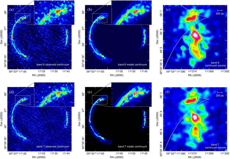
Figure 1: Panels (a) to (c) show the reconstruction of the band 6 continuum image and panels (d) to (f) show the band 7 continuum reconstruction. The observed images are shown in panels (a) and (d), the model images of the reconstructed source are shown in panels (b) and (e) and the reconstructed sources are shown in panels (c) and (f). The white line in the source maps shows the position of the caustic. The inset zooms indicate the fidelity of the reconstruction.

We have verified that these assumptions are valid with the ALMA data analysed in this paper using the following procedure. Firstly, as we discuss below, we located the best fit lens model by application of the semi-linear method in the image plane to the $2\times 2$ binned version of the band 7 continuum image. We then transformed the best fit model lensed image to the $uv$ plane by using MIRIAD uvmodel to produce a simulated visibility dataset for the same $uv$ coverage as in the ALMA dataset. Using the ALMA visibilities, their uncertainties and the model visibilities, we computed $\chi^{2}$. We then varied different lens model parameters, stepping away from the set which provide the best fit in the image plane, generating new images each time and transforming to the $uv$ plane to measure how $\chi^{2}$ varied. We found that although there is a slight offset in parameter space between the image plane minimum-$\chi^{2}$ and the $uv$ plane minimum-$\chi^{2}$, this is within the parameter uncertainties.

3.1 Lens modelling procedure

We used the latest implementation of the semi-linear inversion method (Warren & Dye, 2003) as described by Nightingale & Dye (2015). The crux of the method is the manner in which the source plane discretisation adapts to the magnification produced by a given set of lens model parameters. By introducing a random element to the discretisation and by ensuring that the discretisation maps exclusively back to only those areas in the image within the mask, the method eradicates biases in lens model parameter estimation. Crucially, the method removes a significant bias in the inferred value of the logarithmic slope of power-law mass density profiles which occurs when semi-linear inversion is used with a fixed source plane size and/or a fixed source plane pixellisation (see Nightingale & Dye, 2015, for more details).

We have also used simultaneous reconstruction of multiple source planes from multiple images as described in D14. We attempted a variety of different combinations of data, but found that there were no clear improvements on lens model constraints beyond using a dual reconstruction of the ALMA band 6 and band 7 continuum image data.

For our lens model, we adopted a single smooth power-law profile with a volume mass density of the form $\rho\propto r^{-\alpha}$. In utilising this profile, it is assumed that the power-law slope, $\alpha$, is scale invariant. This assumption appears to be reasonable on the scales probed by strong lensing as demonstrated by a lack of any trend in slope with the ratio of Einstein radius to effective radius (Koopmans et al., 2006; Ruff et al., 2011).

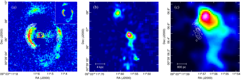
Figure 2: Source reconstruction of the HST F160W data. Panel (a) shows the observed image (note that the residual noise left from lens galaxy light subtraction is masked out in the lens modelling) with band 6 continuum contours overlaid and the inset panel shows the lensed image of the reconstructed source. In panel (b) we show the full scale of the reconstructed source that fits the tidal debris-like emission seen in the observed image. Finally, panel (c) shows a zoomed-in section of the source overlaid with band 6 continuum source contours.

The corresponding projected mass density profile used to calculate lens deflection angles is therefore the elliptical power-law profile introduced by Kassiola & Kovner (1993) with a surface mass density, $\kappa$, given by

$$\kappa=\kappa_{0}\,({\tilde{r}}/{\rm 1kpc})^{1-\alpha}\,.$$ (1)

Here, $\kappa_{0}$ is the normalisation surface mass density (the special case of $\alpha=2$ corresponds to the singular isothermal ellipsoid, SIE). The radius ${\tilde{r}}$ is the elliptical radius defined by ${\tilde{r}}^{2}=x^{\prime 2}+y^{\prime 2}/\epsilon^{2}$ where $\epsilon$ is the lens elongation defined as the ratio of the semi-major to semi-minor axes. Three further parameters define the lens mass profile: the orientation of the semi-major axis measured in a counter-clockwise sense from north, $\theta$, and the coordinates of the centre of the lens in the image plane, $(x_{c},y_{c})$. Finally, following the findings of D14, we include an external shear component which is described by the shear strength $\gamma$ and orientation $\theta_{\gamma}$ measured counter-clockwise from north.

As this paper is concerned primarily with the properties of the lensed source, we have not considered more complicated lens models. For example, one possibility is to model the lens using a cored density profile. Whilst there is continuum emission detected at the centre of the ring where a core would be expected to produce an image, our measurements of the spectral index indicate that this emission cannot be entirely from the background source. Similarly, the high resolution and high signal-to-noise submm images may provide a perfect test-bed for lens mass profiles including substructure. Nevertheless, we leave more detailed lens modelling for future study.

4 Results

4.1 Lens model

Table 1 lists the most probable lens model parameters identified by marginalising over the Bayesian evidence (see Nightingale & Dye, 2015, for more details). The parameters are consistent with those obtained by D14 from modelling solely the HST data. They are also in agreement with the parameters obtained by Rybak et al. (2015) who performed $uv$ modelling of the same ALMA data we have analysed in the present work. This provides further strength to our argument concerning the viability of lens modelling in the image plane in this case.

Lens parameter	Value
$\kappa_{0}$	$(0.86\pm 0.04)\times 10^{10}$M⊙kpc-2
$\epsilon$	$1.25\pm 0.04$
$\theta$	$13^{\circ}\pm 2^{\circ}$
$\alpha$	$2.01\pm 0.05$
$\gamma$	$0.04\pm 0.01$
$\theta_{\gamma}$	$-4^{\circ}\pm 3^{\circ}$

Table 1: Most probable lens model parameters. The quantities are the lens mass normalisation, $\kappa_{0}$, the elongation of the lens mass profile, $\epsilon$, the orientation of the semi-major axis of the lens measured counter-clockwise from north, $\theta$, the density profile slope, $\alpha$, the strength of the external shear component, $\gamma$ and the orientation of the shear $\theta_{\gamma}$ measured counter-clockwise from north.

We also note that the ring is remarkably well fit if we force a slope of $\alpha=2$ and zero external shear, corresponding to a pure SIE model. In this case, the best fit elongation increases to $\epsilon\simeq 1.4$ but the model has a lower evidence (with $\Delta\chi^{2}\simeq 20$) than the most probable model.

Figure 3: Zeroth moment CO maps for C0(5-4) (panel a) and CO(8-7) (panel b) emission in the source, clipped at $2\sigma$. In both maps, the band 6 continuum emission is shown by the white contours and the F160W emission is shown by the yellow contours to illustrate the offset between the different wavelengths.

4.2 Source morphology

Figure 1 shows the lensed source reconstructed from the ALMA band 6 and band 7 continuum images. In the figure, we show the source reconstructed on a regular grid for purposes of illustration, although the adaptive source pixellisation scheme was used in the lens modelling. We also show a zoomed-in section of the image of the source to demonstrate the quality of the fit.

The source continuum emission shows that the distribution of dust is very irregular with many small scale clumps. The morphology is broadly similar between both bands, although the ratio of the band 7 flux to the band 6 flux varies slightly across the source, most likely due to varying dust temperature. Rybak et al. (2015) also show that the star formation rate varies considerably across the source.

Turning to the F160W data, Figure 2 shows our reconstruction performed using the best fit lens model obtained by simultaneously fitting to the band 6 and band 7 continuum data. As is immediately apparent from a direct comparison of the observed lensed images, there is a very distinct offset between the submm emission and the near-IR (rest frame blue) emission. The additional structure revealed by our re-processing of the F160W data is reconstructed in the source plane as shown in panels (b) and (c) of Figure 2. Panel (c) in the figure reveals the dominant near-IR component which gives rise to the bulk of the light seen in the ring. This matches that reconstructed by D14, although a tail of emission to the south is now apparent. In the larger scale reconstruction shown in panel (b), it appears that this tail is only part of a larger extent of near-IR emission. In addition, to the north of the main source component, there is another single component which, in the image plane, gives rise to the arclet seen to the north of the ring. We have measured the F110W-F160W colour of these additional components, drawing on the shallower F110W data described in N14, and find that it is consistent with the colour of the main arc seen in the HST data.

We find total magnification factors of $16.0\pm 0.7$ and $15.8\pm 0.7$ for the band 7 continuum and band 6 continuum reconstructed sources respectively. For the F160W source, we find a total magnification factor of $4.5\pm 0.3$ for the entire source as shown in panel (b) of Figure 2. For the dominant component seen in the F160W source, shown in panel (c) of Figure 2, we measure a magnification factor of $10.2\pm 0.5$, consistent with the magnification measured by D14 for this part of the source.

4.3 CO emission and source kinematics

We used our best fit lens model to reconstruct the distribution of flux in the source plane for each slice of the image data cubes released as part of the ALMA science verification data. Our reconstruction was able to detect significant CO(5-4) and CO(8-7) emission in the reconstructed band 4 and 6 cubes respectively. We were unable to detect any significant CO(10-9) emission in the reconstructed band 7 cube.

Figure 3 shows the zeroth moment map of the CO line emission. These were made using CASA immoments, stacking over channels 31 to 61 inclusive (rest-frame velocities from -370 kms^-1 to 260 kms^-1) for CO(5-4) and channels 30 to 60 inclusive (rest-frame velocities from -391 kms^-1 to 239 kms^-1) for CO(8-7). The channel ranges were selected to fully encompass the spectral range of detected CO emission from the source. Our modelling yields total magnification factors of $13.7\pm 0.6$ for the CO(5-4) flux and $13.1\pm 0.6$ for the CO(8-7) flux.

For comparison, in the zeroth moment maps we also show the the band 6 continuum reconstructed source (white contours) and the F160W source (yellow contours). It is immediately apparent from these plots that while the CO(5-4) emission follows the continuum emission, there is a significant offset between the more highly excited CO(8-7) emission and the continuum. Furthermore, the CO(8-7) map shows more extended emission, linking the submm and near-IR emission regions.

Using CASA immoments to generate a first moment map to obtain the velocity field in each reconstructed CO cube, we also found a relatively smooth variation in velocity across the source (see Figure 4). The velocity field in each cube has the hallmarks of disk rotation and hence we fitted rotation curves assuming rotation of a disk (see Section 4.3.1). Similar application of CASA immoments to generate the second moment map, shows a velocity dispersion which peaks in the dynamical centre of the source but also has strong peaks throughout.

4.3.1 Dynamical modelling

To model the velocity field of the CO(8-7) and CO(5-4) and so estimate the disk inclination and asymptotic rotational velocity, we fitted a two dimensional model whose velocity field is described by a combination of stars and gas such that $v^{2}\,=\,v^{2}_{D}\,+\,v^{2}_{H}$ where the subscripts denote the disk and dark matter halo respectively (we ignore any contribution of Hi to the rotational velocity). For the disk, we assumed that the surface density follows a Freeman profile (Freeman 1970). For the halo, we assumed the Berkert (1995) density profile which incorporates a core of size $r_{0}$ and converges to the Navarro, Frenk & White (1996, NFW) profile at large radii. For suitable values of $r_{0}$, the Berkert profile can mimic the NFW or an isothermal profile over the limited region of galaxy mapped by the rotation curves.

This mass model has three free parameters: the disk mass, the core radius of the dark matter halo and the central core density. To fit the two-dimensional velocity fields, we constructed a two-dimensional kinematic model with these three parameters, but we also we allowed the [$x$ / $y$] centre of the disk, the position angle (PA) and the disk inclination to be additional free parameters. We constrained the [$x$ / $y$] dynamical centre to be within 0.5 kpc of the band 7 continuum centroid and then fitted the two dimensional dynamics using an MCMC code (see Swinbank et al., 2012, for further details)

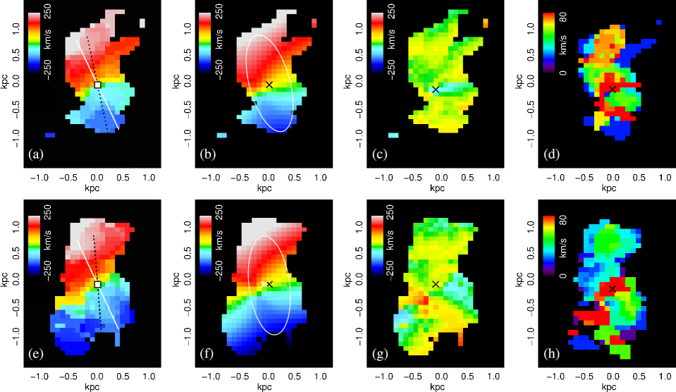
Figure 4: Observed, modelled and residual velocity fields (panels (a), (b) and (c) respectively) and observed line of sight velocity dispersion (panel d) for the CO(8-7) line emission. The same quantities in the same order are shown for the CO(5-4) emission in panels (e) to (h). The white line in panels (a) and (e) shows the principle axis of the best-fit disk model and the dashed black line shows that of the stacked CO emission. The white ellipse in panels (b) and (f) shows the extent of the disk used in the dynamical modelling.

The best-fit kinematic maps and velocity residuals are shown in Figure 4. The best fit disk inclination is $(40\pm 5)^{\circ}$. Assuming that the observed velocity field is indeed due to disk rotation, then the observed maximum line of sight rotational velocity of 210 kms^-1 corresponds to an intrinsic asymptotic velocity of 320 kms^-1.

Figure 5 shows the one dimensional rotation curves extracted from a 0.4 kpc wide strip running along the major kinematic axis identified from the dynamical models for the CO(8-7) and CO(5-4) emission. For these rotation curves, we defined the velocity zero point using the dynamical centre of the galaxy. The error bars for the velocities are derived from the formal $1\sigma$ uncertainty in the velocity arising from the Gaussian profile fits to the CO emission. We note that the data have not been folded about the zero velocity, so that the degree of symmetry can be assessed.

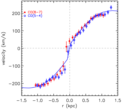
Figure 5: Rotation curves of the lensed source from CO(5-4) and CO(8-7) emission, strongly resembling disk-like dynamics in both cases. The data points show the observed line of sight velocity extracted from a 0.4 kpc wide slit running along the major kinematic axis and the line shows the best dynamical model fit.

The rotation curves imply a mass within 1.5 kpc of $(3.5\pm 0.5)\times 10^{10}$ M_⊙ with only a small contribution from the halo within this radius. Comparing the significantly lower maximum velocity dispersion of $\sim 90$ kms^-1 with this rotational velocity suggests, under the assumption of a disk, that a correction for asymmetric drift need not be applied to the inferred dynamical mass. If we assume that all of the mass lies within the exponential disk component, this corresponds to a surface mass density of $5000\pm 900$ M_⊙pc^-2. This is a typical value for high redshift SMGs (see Figure 6 in Ivison et al., 2013).

Using this surface mass density and the observed velocity dispersion in the disk, the resulting Toomre stability value is $Q\simeq 0.3$ which indicates a collapsing disk. Such low values of $Q$ are observed in early merger systems before feedback can restore equilibrium in the disk (see Hopkins, 2012).

4.4 Other intrinsic source properties

4.4.1 Dust mass and total dust luminosity

We have measured the dust mass of the lensed source by fitting a two-component spectral energy distribution (SED) model to a combination of our measured band 6 and band 7 continuum fluxes and also the source fluxes presented in N14 but de-magnified by our average continuum magnification factor of 15.9. The SED model allows the dust temperature, emissivity index, $\beta$, and optical depth at 100 $\mu$m, $\tau_{100}$, to vary in the fitting. We used a dust mass opacity coefficient equivalent to $\kappa_{850\mu{\rm m}}=0.077$ m² kg^-1 to be consistent with the fitting in N14.

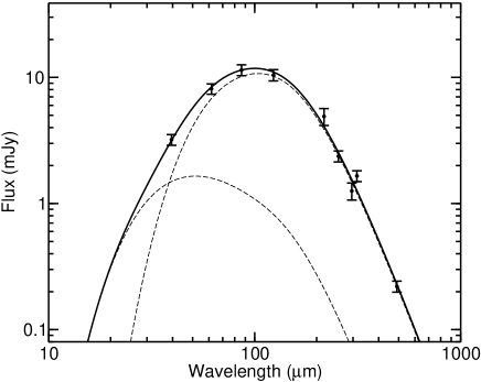
Figure 6: Rest-frame de-magnified best fit SED to the band 6 and 7 continuum source fluxes and to the fluxes from table 2 in N14 (but de-magnified using our derived continuum source magnification factor). The dashed curves show the hot (99 K) and cold (48 K) SED components.

Figure 6 shows the best fit SED model which has an effective dust temperature of 51 K, an emissivity index of $\beta=2.5$ and an optical depth of $\tau_{100}=6.5$, yielding a dust mass of $(1.8\pm 0.3)\times 10^{8}$ M_⊙ after de-magnifying by our average continuum magnification factor. The fit favours both a hot and cold dust component with temperatures of 99 K and 48 K respectively.

If we fix the emissivity index to $\beta=2.0$, we obtain a lower optical depth of $\tau_{100}=3$ and a lower temperature of 46 K but all optically thick fits, with or without fitting to the 160$\mu$m flux (which corresponds to rest-frame $\sim 40\,\mu$m and therefore not well fit by a modified black body SED) returned a dust mass in the range $(1.8-2.1)\times 10^{8}$ M_⊙. A second colder dust temperature component (10–40 K) was allowed in the fitting but was not favoured by the data.

Assuming a typical gas to dust ratio of 150 (for example Dunne et al., 2000; Draine et al., 2007; Coretese et al., 2012; Sandstrom et al., 2013; Swinbank et al., 2014) therefore gives a total molecular gas mass of $(2.7\pm 0.5)\times 10^{10}$ M_⊙. In making these calculations, we have of course neglected any effects of differential magnification which could bias the inferred dust temperature and/or emissivity index.

From integrating the best-fit SED between 8 and 1000 $\mu$m, we estimate that the total far-infrared emission is $(5.0\pm 0.8)\times 10^{13}$ L_⊙, which agrees well with the value of $5.4\times 10^{13}$ L_⊙ given in N14. Our estimate of the average continuum magnification factor of 15.9 implies that the intrinsic far-infrared luminosity is $(3.1\pm 0.5)\times 10^{12}$ L_⊙.

4.4.2 CO(1-0) gas

We have derived an estimate of the CO(1-0) luminosity of the gas in the lensed source using the CO(1-0) spectroscopic data acquired by Valtchanov et al. (2011). To do this, we firstly determined the spectrum of the total lensed flux (note that Valtchanov et al. plot the peak spectrum in their work). We then used our CO(5-4) source plane velocity and the magnification map from the lens model to estimate the magnification as a function of velocity in the source plane. By transforming the total CO(1-0) SED to velocity space, we then de-magnified the SED flux at each velocity with the corresponding magnification factor from our magnification-velocity relation. Figure 7 shows the de-magnified SED.

Using the de-magnified SED, we determined a CO(1-0) flux of $f_{\rm CO(1-0)}=85\pm 12$ mJy kms^-1, which corresponds to a luminosity of L${}^{\prime}_{\rm CO}=(3.5\pm 0.6)\times 10^{10}$ K kms^-1 pc². The errors take into account a number of uncertainties: 1) There appears to be more CO(1-0) emission at higher and lower velocities than we see in our CO(5-4) data and so in our velocity-magnification relationship, we assumed a fixed magnification of 3 in these extremes; 2) The measure of de-magnified flux is sensitive to the binning of the CO(1-0) spectrum and velocity-magnification mapping; 3) We have determined the de-magnified flux assuming the CO(1-0) emission exactly follows the CO(5-4) emission. The flux changes by $\sim 15\%$ if we assume the CO(1-0) emission is more evenly distributed in the source plane.

To estimate the total mass of molecular gas in the source, we used the CO luminosity to molecular gas mass conversion factor from Bothwell et al. (2013) of $\alpha_{\rm CO}=1$ (although there is a very large uncertainty on this factor; see for example Papadopoulos et al., 2012). This gives a total molecular gas mass in the source of $(3.5\pm 0.6)\times 10^{10}$ M_⊙ which is larger than the value of $(2.7\pm 0.5)\times 10^{10}$ M_⊙ we obtained by scaling from the dust mass, although both come with considerable uncertainty depending on the choice of assumptions (e.g., the dust-to-gas ratio, or the minimum amplification for gas beyond that seen in CO(5-4)). Nevertheless, using the dynamical mass as an estimate of the total mass, and the range of gas masses derived from either the CO(1-0) or the dust luminosity, these values suggest a high molecular gas fraction in the central regions, in the range $\sim 75-100$ per cent.

5 Discussion

Figure 7: The de-magnified CO(1-0) spectrum in velocity space. The unshaded red histogram shows our estimated magnification factor.

The offset between the reconstructed rest-frame optical source emission detected by HST/WFC3 and the reconstructed submm source from the ALMA data is striking. D14 found good alignment between the rest-frame optical emission and the submm source reconstructed by Bussmann et al. (2013), although this latter study used imaging acquired with The Submillimeter Array (SMA) with a beam width approximately two orders of magnitude larger than the ALMA image data analysed in the present work. The anti-correlation seen between the rest-frame optical and submm emission is not unique; the configuration in SDP.81 is similar to the offset between the optical and submm emission seen in the z=4.05 SMG GN20 (see Daddi et al., 2009; Hodge et al., 2015). However, occurrence of such large offsets is not common. For example, in a survey of 126 SMGs carried out using ALMA (see Hodge et al., 2013), only two sources, ALESS88.11 and ALESS92.2 exhibit a similar configuration (Chen et al., 2015).

There are a number of scenarios which could explain the observed configuration of the lensed source. The three most likely ones are: 1) The submm and optical components are simply two different sources which are closely aligned on the sky but well separated along the line of sight; 2) The submm and optical emission originates from the same source and we observe a total lack of optical emission from the submm region due to very strong dust absorption; 3) The optical and submm components are two separate systems undergoing a merger.

The first scenario is challenging to verify, not least because of the large effective radius of the lens in the optical/near-infrared compared to the Einstein radius for the optical source. Photon noise from the lens light thus dominates the already faint optical source which will hinder attempts to measure its redshift, either spectroscopically or photometrically. This scenario also draws into question the structure of the optical source and the nature of the apparent tidal debris to the south and the component to the north.

The second scenario could arise as a result of a strong dust lane in a disk galaxy. There are many examples of ULIRGs in the local Universe where strong absorption by dust lanes result in a delineation between optical and submm emission. In the case of SDP.81, it may be that a wide and thick dust lane is located at the eastern edge of the disk, which, because of its inclination, provides a much higher column density of dust toward regions in the source which emit optically. On the assumption that the optical absorption efficiency factor of a dust grain is inversely proportional to wavelength, which is true in Mie theory if the grain size is much less than the wavelength, our estimate of the optical depth at 100 $\mu$m (see Section 4.4.1) implies that the optical depth in the optical waveband is $\sim 1000$. Therefore, we would not expect to see much starlight from within the disk of gas and dust.

The third scenario is suggested by the presence of the northern rest-frame optical component and the apparent tidal debris seen to the south. A tempting interpretation of this is that the northern component is a second galaxy which has passed through the larger, strongly lensed system, causing the tidal debris observed and enhancing the star formation rate and dust mass. Although the velocity field appears to be quite regular, the low Toomre Q parameter we have measured ($Q\simeq 0.3$) suggests a collapsing disk. Also, there are several strong peaks in the velocity dispersion map which may still point towards some level of interaction and there are filaments in the CO(8-7) emission (but not the less excited CO(5-4) emission) which extend up to the optical region. The strong emission in CO(8-7) is itself consistent with a merger scenario since this higher energy transition can not be produced over the entire observed disk by UV flux from star formation (Papadopoulos et al., 2014).

In our attempts to search for more hints as to the nature of the source, we also carefully searched through all channels in the band 6 and 7 ALMA data cubes, looking for CO emission from the northern and southern optical components. Such emission might indicate an association with the source or provide additional kinematic information. We could not find any significant emission from the northern or southern optical components in either of the cubes.

Whatever the connection between the rotating disk of gas and dust revealed by ALMA and the HST near-infrared sources, we can draw some conclusions about the properties of the star formation in the disk. We have estimated the star-formation rate in the disk from the intrinsic far-infrared luminosity, which is the method suggested by Kennicutt & Evans (2012) for estimating the star-formation rate in a highly obscured galaxy. From the relationship between star-formation rate and far-infrared luminosity given in Kennicutt & Evans, we estimate that the star-formation rate in this object is $\sim 470\pm 80$ M_⊙/yr.

Source property	Value
Total continuum magnification	$15.9\pm 0.7$
Total rest-frame optical magnification	$10.2\pm 0.5$
Total CO(5-4) magnification	$13.7\pm 0.6$
Total CO(8-7) magnification	$13.1\pm 0.6$
Disk inclination	$(40\pm 5)^{\circ}$
Asymptotic rotational velocity	320 kms-1
Toomre Q Parameter	0.3
Total dust mass	$(1.8\pm 0.3)\times 10^{8}$ M⊙
Total molecular gas mass from dust	$(2.7\pm 0.5)\times 10^{10}$ M⊙
Dynamical mass within 1.5 kpc	$(3.5\pm 0.5)\times 10^{10}$ M⊙
Total CO luminosity	L${}^{\prime}_{\rm CO}=(3.5\pm 0.6)\times 10^{10}$ K km s-1 pc2
Total molecular gas mass from CO	$(3.5\pm 0.6)\times 10^{10}$ M⊙
Star-formation rate	$470\pm 80$ M⊙/yr
CO(1-0) flux	$34\pm 5$ mJy kms-1
Total far-infrared luminosity	$(3.1\pm 0.5)\times 10^{12}$ L⊙

Table 2: Summary of the intrinsic (i.e. de-magnified where relevant) physical properties of the source.

Although it is well-known that high-redshift galaxies are very clumpy and irregular in broad-band optical/UV images (Cowie, Hu & Songalia, 1995), it has always been an open question whether the clumpiness is the result of the star formation occurring in clumps or whether it is the result of patchy dust obscuration. In the case of this object, both the reconstructed CO and dust emission are clumpy on the scale of the point spread function in the reconstructed images, $\sim 200$ pc. The CO lines are high-excitation lines, so that we cannot rule out the possibility that the clumpiness is the result of a variation in the excitation rather than a variation in the distribution of the gas. There is also the recent suggestion that a clumpy CO distribution in high-redshift galaxies might be the result of the destruction of CO molecules by cosmic rays (Bisbas, Papadopoulos & Viti, 2015). However, neither of these two caveats apply to the dust emission; dust grains are robust and found in all phases of the interstellar medium, and the emission from the dust depends only very weakly on the intensity of the interstellar radiation field. Therefore, the clumpiness of the dust is strong evidence that the distribution of gas in this object is truly extremely clumpy. The low value of the Toomre Q parameter and the very irregular distribution of gas are exactly what one would expect if sections of the disk are collapsing to form stars. From the rotation curve and the velocity dispersion, we estimate that the disk is unstable over the scale range $\sim 50$ pc to $\sim 700$ pc, the lower limit being the Jeans length and the upper limit being the scale on which the disk should be stabilised by shear. This agrees well with the sizes of the clumps observed.

Finally, we have estimated the efficiency of the star-formation process in this galaxy. Using the dust mass as a tracer of the total mass of gas, Rowlands et al. (2014) and Santini et al. (2014) have found evidence that the star-formation efficiency (star-formation rate/gas mass) is higher in high-redshift galaxies than in galaxies in the local Universe. Rowlands et al. (2014) give relationships between the star-formation rate and dust mass for local galaxies and for high-redshift SMGs. Using these relationships, we estimate that a typical galaxy in the local Universe with a dust mass equal to that of SDP.81 would be forming stars at a rate of $7.2\pm 1.3$ M_⊙/yr and that a typical SMG with the same dust mass would be forming stars at a rate of $58\pm 10$ M_⊙/year. Thus our estimated SFR of SDP.81 of 470 M_⊙/yr implies a star formation efficiency that is $\sim 8$ times greater than a typical SMG and $\sim 65$ times greater than in the nearby Universe.

6 Summary

We have used the exceptional angular resolution of ALMA to reconstruct a detailed map of the submm emission and dynamics in the lensed source in SDP.81. Our modelling of the reprocessed HST data has revealed an offset of $\sim 1.5$ kpc between the submm and rest-frame optical centroids in the source. The submm continuum emission in the source is magnified by a total magnification factor of $15.9\pm 0.7$ which compares to the magnification of the rest-frame optical emission of $10.2\pm 0.5$ which mainly lies outside of the source plane caustic. Similarly, the CO(5-4) and CO(8-7) emission is magnified by the total magnification factors $13.7\pm 0.6$ and $13.1\pm 0.6$ respectively.

Our reconstruction of the source kinematics from the CO emission reveals a relatively smooth velocity gradient across the source and suggests regular disk-like rotation. We have carried out dynamical modelling of the observed line of sight velocities and find that the data are best fit by a disk inclined at an angle of $(40\pm 5)^{\circ}$ to the line of sight with an asymptotic rotational line of sight velocity of 210 kms^-1. Accounting for the disk inclination, this corresponds to an intrinsic asymptotic velocity of 320 kms^-1 and an implied dynamical mass of $(3.5\pm 0.5)\times 10^{10}$ M_⊙ within 1.5 kpc. Our dynamical modelling returns a low Toomre Q-parameter of $Q\simeq 0.3$.

We have combined our measurements of the dust continuum flux from the ALMA data with photometry of the lensed source given in Negrello et al. (2014) to fit a modified black body SED. This indicates a total dust mass of $(1.8\pm 0.3)\times 10^{8}$ M_⊙ after de-magnifying by our average continuum magnification factor. Assuming a typical gas to dust ratio of 150 gives total molecular gas mass of $(2.7\pm 0.5)\times 10^{10}$ M_⊙. We have also estimated the total molecular gas mass from the de-magnified CO(1-0) spectrum of the lensed source from Valtchanov et al. (2011). This gives a total CO luminosity of L${}^{\prime}_{\rm CO}=(3.5\pm 0.6)\times 10^{10}$ K km s^-1 pc² which, assuming a gas mass conversion factor of unity, typical for ULIRGs in the local Universe, gives a total molecular gas mass of $(3.5\pm 0.6)\times 10^{10}$ M_⊙.

One observable we have not discussed in this work is the low-excitation water line H₂O$~{}(2_{\rm 02}-1_{\rm 11}$) ($v_{\rm rest}$ = 987.927 GHz ($E_{\rm up}$ = 101 K)) which can be seen in the band 6 data. We have attempted to reconstruct the distribution of this line in the source plane using our most probable lens model, but this has proven too weak to locate easily. We have therefore left analysis of this feature for future study.

To summarise, the nature of SDP.81 is somewhat perplexing! Although the observational evidence we have assembled in this paper is suggestive of a galaxy merger, we cannot rule out other possibilities. Pending further analysis of additional observational data, the source evades our full understanding. Nevertheless, this work has demonstrated the complexity we can begin to expect in high redshift SMGs when they are studied at the high angular resolution now made possible by ALMA’s incredible long baseline imaging capability.

References

- Ahn et al. (2014) Ahn, C. P., et al., 2014, ApJS, 211, 17
- Alaghband-Zadeh et al. (2012) Alaghband-Zadeh, S., et al., 2012, MNRAS, 424, 2232
- ALMA Partnership, Vlahakis et al. (2015) ALMA Partnership, Vlahakis, C., et al., 2015, ApJL in press, arXiv:1503.02652
- Barger et al. (1998) Barger, A. J., Cowie, L. L., Sanders, D. B., Fulton, E., Taniguchi, Y., Sato, Y., Kawara, K., Okuda, H., 1998, Nature, 394, 248
- Berkert (1995) Berkert, A., 1995, ApJ, 447, 25
- Bisbas, Papadopoulos & Viti (2015) Bisbas, T.G., Papadopoulos, P. & Viti, S., 2015, ApJ in press, arXiv:150204198
- Blain (1996) Blain, A. W., 1996, MNRAS, 283, 1340
- Bothwell et al. (2013) Bothwell, M. S., et al., 2013, MNRAS, 429, 3047
- Bournaud & Elmegreen (2009) Bournaud, F. & Elmegreen, B. G., 2009, ApJL, 694, L158
- Bussmann et al. (2013) Bussmann, R. S. et al., 2013, ApJ, 779, 25
- Carlstrom et al. (2011) Carlstrom, J., E., et al., 2011, PASP, 123, 568
- Chen et al. (2015) Chen, C. -C., et al., 2015, ApJ, 799, 194
- Coretese et al. (2012) Cortese, L., et al., 2012, A&A, 540, 52
- Cowie, Hu & Songalia (1995) Cowie, L. L., Hu, E. M. & Songaila, A., 1995, AJ, 110, 1576
- Daddi et al. (2009) Daddi, E., et al., 2009, ApJ, 694, 1517
- Downes & Salomonv (1998) Downes, D. & Solomon, P. M., 1998, ApJ, 507, 615
- Draine et al. (2007) Draine, B. T., et al., 2007, ApJ, 663, 866
- Dunne et al. (2000) Dunne, L., Eales, S. A., Edmunds, M., Ivison, R., Alexander, P., Clements, D. L., 2000, MNRAS, 315, 115
- Dye et al. (2014) Dye, S., 2014, MNRAS, 440, 2013, D14
- Eales et al. (2010) Eales et al., 2010, PASP, 122, 499
- Engel et al. (2010) Engel, H., et al., 2010, ApJ, 724, 233
- Fixsen et al. (1998) Fixsen, D. J., Dwek, E., Mather, J. C., Bennett, C. L., Shafer, R. A., 1998, ApJ, 508, 123
- Hezaveh & Holder (2011) Hezaveh, Y. D. & Holder, G. P., 2011, ApJ, 734, 52
- Hodge et al. (2013) Hodge, J. A., et al., 2013, ApJ, 768, 91
- Hodge et al. (2015) Hodge, J. A., Riechers, D., Decarli, R., Walter, F., Carilli, C. L., Daddi, E., Dannerbauer, H., 2015, ApJ, 798, L18
- Hopkins (2012) Hopkins, P. F., 2012, MNRAS, 423, 2037
- Hughes et al. (1998) Hughes, D. H., et al., 1998, Nature, 394, 241
- Ivison et al. (2013) Ivison, R. J., et al., 2013, ApJ, 772, 137
- Jones et al. (2010) Jones, T., Ellis, R., Jullo, E., Richard, J., 2010, ApJL, 725, L176
- Kassiola & Kovner (1993) Kassiola, A. & Kovner, I., 1993, ApJ, 417, 450
- Kennicutt & Evans (2012) Kennicutt, R. & Evans, N. J., 2012, ARAA, 50, 531
- Koopmans et al. (2006) Koopmans, L. V. E., Treu, T., Bolton, A. S., Burles, S., Moustakas, L. A., 2006, ApJ, 649, 599
- Krist (1993) Krist, J. E., 1993, Astronomical Data Analysis Software and Systems II, A.S.P. Conference Series, Vol. 52, eds. R. J. Hanisch, R. J. V. Brissenden, and Jeannette Barnes, p. 536
- McMullin et al. (2007) McMullin, J. P., Waters, B., Schiebel, D., Young, W., Golap, K., 2007, in ASP Conf. Ser. 376, Astronomical Data Analysis Software and Systems XVI, eds. R. A. Shaw, F. Hill, & D. J. Bell (San Francisco, CA: ASP), 127
- Navarro, Frenk & White (1996) Navarro, J. F., Frenk, C. S. & White S. D. M., 1996, ApJ, 462, 563
- Negrello et al. (2007) Negrello, M., Perrotta, F., González-Nuevo, J., Silva, L., de Zotti, G., Granato, G. L., Baccigalupi, C., Danese, L., 2007, MNRAS, 377, 1557
- Negrello et al. (2010) Negrello, M., et al., 2010, Science, 330, 800
- Negrello et al. (2014) Negrello, M., et al., 2014, MNRAS, 440, 1999, N14
- Nightingale & Dye (2015) Nightingale, J. W. & Dye, S., 2015, MNRAS submitted, arXiv:1412.7436
- Oliver et al. (2012) Oliver, S. J., et al., 2012, MNRAS, 424, 1614
- Papadopoulos et al. (2011) Papadopoulos, P. P., Thi, W.-F., Miniati, F., Viti, S., 2011, MNRAS, 414, 1705
- Papadopoulos et al. (2012) Papadopoulos, P. P., van der Werf, P., Xilouris, E., Isaak, K. G., Gao, Y., 2012, ApJ, 751, 10
- Papadopoulos et al. (2014) Papadopoulos, P. P., et al., 2014, ApJ, 788, 153
- Peng et al. (2002) Peng, C. Y., Ho, L. C., Impey, C. D., Rix, H. -W., 2002, AJ, 124, 266
- Planck Collaboration (2014) Planck Collaboration; Ade, P., et al., 2014, A&A, 571, 26
- Puget et al. (1996) Puget, J. L., Abergel, A., Bernard, J.P., Boulanger, F., Burton, W. B., Desert, F.-X., Hartmann, D., 1996, A&A, 308, L5
- Rowlands et al. (2014) Rowlands, K., et al., 2014, MNRAS, 441, 1017
- Ruff et al. (2011) Ruff, A. J., Gavazzi, R., Marshall, P. J., Treu, T., Auger, M. W., Brault, F., 2011, ApJ, 727, 96
- Rybak et al. (2015) Rybak, M., McKean, J. P., Vegetti, S., Andreani, P., White, S. D. M., 2015, MNRAS submitted, arXiv:1503.02025
- Sandstrom et al. (2013) Sandstrom K. M., et al., 2013, ApJ, 777, 5
- Santini et al. (2014) Santini, P., et al., 2014, A&A, 562, 30
- Smail et al. (1997) Smail, I., Ivison, R. J., Blain, A. W., 1997, ApJ, 490, L5
- Skrutskie et al. (2006) Skrutskie, M. F., et al., 2006, AJ, 131, 1163
- Swinbank et al. (2010) Swinbank, A. M., et al., 2010, MNRAS, 405, 234
- Swinbank et al. (2012) Swinbank, A. M., Smail, Ian, Sobral, D., Theuns, T., Best, P. N., Geach, J. E., ApJ, 760, 130
- Swinbank et al. (2014) Swinbank, A. M., et al., 2014, MNRAS, 438, 1267
- Valtchanov et al. (2011) Valtchanov, I., et al., 2011, MNRAS, 415, 3473
- Vieira et al. (2010) Vieira, J. D., et al., 2010, ApJ, 719, 763
- Vieira et al. (2013) Vieira, J. D., et al., 2013, Nature, 496, 344
- Warren & Dye (2003) Warren, S. J. & Dye, S., 2003, ApJ, 590, 673
- Wardlow et al. (2013) Wardlow, J. L., et al., 2013, ApJ, 762, 59