Quench dynamics and ground state fidelity of the one-dimensional extended quantum compass model in a transverse field

Abstract

We study the ground state fidelity, fidelity susceptibility and quench dynamics of the extended quantum compass model in a transverse field. This model reveals a rich phase diagram which includes several critical surfaces depending on exchange couplings. We present a characterization of quantum phase transitions in terms of the ground state fidelity between two ground states obtained for two different values of external parameters. However, we derive scaling relations describing the singular behavior of fidelity susceptibility in the quantum critical surfaces. Moreover, we study the time evolution of the system after a critical quantum quench using the Loschmidt. We find that the revival times of Loschmidt echo are given by $T_{rev}=N/2v_{max}$, where $N$ is the size of the system and $v_{max}$ is the maximum of lower bound group velocity of quasi-particles. Although the fidelity susceptibility shows the same exponent in all critical surfaces, the structure of the revivals after critical quantum quenches displays two different regimes reflecting different equilibration dynamics.

I Introduction

In the last few years a big effort has been assigned to the analysis of quantum phase transitions (QPTs) from the perspective of quantum information Osterloh ; Vidal ; Osborne ; kargarian1 ; kargarian2 ; Jafari1 ; kargarian3 ; Jafari2 ; Langari ; Jafari ; Mehran ; Jafari5 . Entanglement and fidelity have been accepted as new notions to characterize quantum phase transitions. Entanglement, referring to quantum correlations between subsystems is a good indicator of quantum phase transitions, because the correlation length diverges at the quantum critical points Osterloh ; Vidal ; Osborne . The fidelity which is a measure of distance between quantum states, could be also a nice tool to study the drastic change in the ground states in quantum phase transitions Zanardi .

On the other hand, recent advances in the studies of ultra-cold atoms trapped in optical lattices introduced a new tool to simulate the dynamics of interacting quantum many-body systems in non-equilibrium strongly correlated quantum systems Greiner ; Jaksch . These new opportunities are concentrated by the pioneering experiments on tunable Mott insulator to superfluid quantum phase transitions, observed by utilization of the optical lattice potential in three-dimensional 3D Greiner and 1D Stoferle systems.

Recently the investigation of non-equilibrium properties of closed quantum systems have been getting a lot of attention for several reasons. Specifically it has been applied to quantum information in which decoherence and entanglement dynamics play an essential role. From the theoretical point of view, it is very important to understand the notion of universality for a system away from equilibrium, where the traditional concepts of phase, fixed point and renormalization group fail. Driving a system out of equilibrium is done in many ways. Most of the attention has been focused on quantum quenches Chandra , namely, sudden changes of the external parameters of the Hamiltonian controlling the unitary evolution of the closed system. One of the conventional methods of understanding the dynamics of a system after a quench is the Loschmidt echo (LE), which is a benchmark of the partial or full reappearance of the original state as a function of time Gorin ; Jacquod . The LE is defined as follows: if a quantum state $|\psi\rangle$ evolves with two Hamiltonians $H$ and $H^{\prime}$, respectively, the LE is the measure of the overlap given by $LE=|\langle\psi|\exp(\imath H^{\prime}t)\exp(-\imath Ht)|\psi\rangle|^{2}$. If the system admits the ground state, LE is a dynamical version of the ground state fidelity. Recently, the time behavior of the LE has been studied in well-known models, in particular the $XY$ spin chain Venuti2 ; Quan and cluster XY chain Montes . High values of the LE mean that the system is approaching the initial state. Typically, the LE will decay exponentially at first and then start oscillating around an average value Venuti2 . If the system is finite, the time evolution is quasi-periodic, forcing the system arbitrarily close to the initial state for long enough times. The system will show revivals, i.e., times when the value of the LE is greater than the average value. The structure of these revivals may be greatly influenced by criticality Venuti2 . In this work, the phase diagram and universality of the one-dimensional extended quantum compass model (EQCM) Eriksson ; Mahdavifar ; Motamedifar in a transverse filed Jafari3 ; Jafari4 will be studied by means of the fidelity of the ground state and fidelity susceptibility. This inhomogeneous model covers a group of well-known spin models as its special cases and shows a rich phase diagram. It should be mentioned that the phase diagram Motamedifar , quantum correlation You , bipartite entanglement Liu and fidelity Motamedifar2 , of this model have been studied numerically using the exact diagonalization method and infinite time-evolving block decimation Vidal2 . This study is an important addition to the literature as to the best of our knowledge, the quenches of a Hamiltonian which also undergoes a very unique type of quantum phase transition Eriksson ; Jafari3 ; Jafari4 , has not been investigated before. However, it will be instructive to study the quenches near quantum critical points because of the expected universality of the response of the system, and thus the possibility of using the quench dynamics as a nonequilibrium probe of phase transitions. Then, we will explore the quenching dynamics of this model, when the transverse field or the exchange couplings is quenched.

II The Hamiltonian and its Exact Solution

Consider the Hamiltonian

$$H=\sum_{n=1}^{N^{\prime}}[J_{1}\sigma^{x}_{2n-1}\sigma^{x}_{2n}+J_{2}\sigma^{y}_{2n-1}\sigma^{y}_{2n}+L_{1}\sigma^{x}_{2n}\sigma^{x}_{2n+1}+L_{2}\sigma^{y}_{2n}\sigma^{y}_{2n+1}+h(\sigma^{z}_{2n-1}+\sigma^{z}_{2n})].$$ (1)

where $J_{1}$ and $J_{2}$ are the odd bonds exchange couplings, $L_{1}$ and $L_{2}$ are the even bond exchange couplings and $N=2N^{\prime}$ is the number of spins. It should be pointed out that although periodic and antiperiodic boundary conditions differ in O(1/N) terms, this difference usually does not affect the phase diagram or other quantities in the thermodynamic limit. However, although it can be important in the LE that is typically exponentially small in $N$ and the boundary conditions could have a dramatic effect in the case of the critical quench Happola , but for simplicity we assume periodic boundary conditions. This model embraces a group of the other familiar spin models as its special cases, such as the quantum Ising model in a transverse field for $J_{2}=L_{2}=0$, the transverse field XY model for $J_{1}=L_{1}$ and $J_{2}=L_{2}$, and the transverse field XX model for $J_{1}=J_{2}=L_{1}=L_{2}$. The above Hamiltonian [Eq. (1)] can be exactly diagonalized by standard Jordan-Wigner transformation Jordan ; Jafari3 ; Jafari4 as defined below,

$$\sigma^{x}_{j}=b^{+}_{j}+b^{-}_{j},~{}~{}\sigma^{y}_{j}=b^{+}_{j}-b^{-}_{j},~{}~{}\sigma^{z}_{j}=2b^{+}_{j}b^{-}_{j}-1,~{}~{}b^{+}_{j}=c^{{\dagger}}_{j}~{}e^{i\pi\Sigma_{m=1}^{j-1}c^{{\dagger}}_{m}c_{m}},~{}~{}b^{-}_{j}=e^{-i\pi\Sigma_{m=1}^{j-1}c^{{\dagger}}_{m}c_{m}}~{}c_{j}$$

which transforms spins into fermion operators $c_{j}$.

The crucial step is to define independent Majorana fermions Perk ; Sengupta at site $n$, $c_{n}^{q}\equiv c_{2n-1}$ and $c_{n}^{p}\equiv c_{2n}$. This can be regarded as quasiparticles’ spin or as splitting the chain into bi-atomic elementary cells Perk .

Substituting for $\sigma^{x}_{j}$, $\sigma^{y}_{j}$ and $\sigma^{z}_{j}$ ($j=2n,2n-1$) in terms of Majorana fermions followed by a Fourier transformation, Hamiltonian Eq.(1) (apart from an additive constant), can be written as

$$H^{+}=\sum_{k}\Big{[}Jc_{k}^{q{\dagger}}c_{-k}^{p{\dagger}}+Lc_{k}^{q{\dagger}}c_{k}^{p}+2h(c_{k}^{q{\dagger}}c_{k}^{q}+c_{k}^{p{\dagger}}c_{k}^{p})+h.c.\Big{]},$$

where $J=(J_{1}-J_{2})-(L_{1}-L_{2})e^{ik}$, $L=(J_{1}+J_{2})+(L_{1}+L_{2})e^{ik}$ and $k=\pm\frac{j\pi}{N^{\prime}},~{}(j=1,3,\cdots,N^{\prime}-1)$.

By grouping together terms with $k$ and $-k$, the Hamiltonian is transformed into a sum of independent terms acting in the 4-dimensional Hilbert spaces generated by $k$ and $-k$ ($H^{+}=\bigoplus_{k>0}H_{k}^{+})$, in other word $[H_{k},H_{k^{\prime}}]=0$ in which

$$H_{k} = (Jc_{k}^{q{\dagger}}c_{-k}^{p{\dagger}}+Lc_{k}^{q{\dagger}}c_{k}^{p}-J^{\ast}c_{k}^{q}c_{-k}^{p}-L^{\ast}c_{k}^{q}c_{k}^{p{\dagger}}+Jc_{-k}^{q{\dagger}}c_{k}^{p{\dagger}}+Lc_{-k}^{q{\dagger}}c_{-k}^{p}-J^{\ast}c_{-k}^{q}c_{k}^{p}-L^{\ast}c_{-k}^{q}c_{-k}^{p{\dagger}})$$

$$+ 2h(c_{k}^{q{\dagger}}c_{k}^{q}+c_{k}^{p{\dagger}}c_{k}^{p}+c_{-k}^{q{\dagger}}c_{-k}^{q}+c_{-k}^{p{\dagger}}c_{-k}^{p}).$$

Hamiltonian Eq. (II) can be written in the diagonal block form

$$H=\sum_{k}\Gamma^{{\dagger}}_{k}.A(k).\Gamma_{k}$$ (3)

where $\Gamma^{{\dagger}}_{k}=(c_{k}^{q},c_{-k}^{q{\dagger}},c_{k}^{p},c_{-k}^{p{\dagger}})$ and

$$A(k)=\left(\begin{array}[]{cccc}2h&0&L&J\\ 0&-2h&-J&-L\\ L^{\ast}&-J^{\ast}&2h&0\\ J^{\ast}&-L^{\ast}&0&-2h\\ \end{array}\right).$$ (8)

By using the element of the new vector $\Gamma^{\prime{\dagger}}_{k}=(\gamma_{k}^{q},\gamma_{-k}^{q{\dagger}},\gamma_{k}^{p},\gamma_{-k}^{p{\dagger}})$ which could be described by unitary transformation $\Gamma^{\prime}_{k}=U_{k}\Gamma_{k}$ (see Appendix A), the matrix $A(k)$ can be diagonalized easily and we find the Hamiltonian Eq. (II) in a diagonal form.

$$H=\sum_{k}\Big{[}E^{q}_{k}(\gamma_{k}^{q{\dagger}}\gamma_{k}^{q}-\frac{1}{2})+E^{p}_{k}(\gamma_{k}^{p{\dagger}}\gamma_{k}^{p}-\frac{1}{2})\Big{]},$$ (9)

where $E^{q}_{k}=\sqrt{a+\sqrt{b}}$ and $E^{p}_{k}=\sqrt{a-\sqrt{b}}$, in which

$$a=4h^{2}+|J|^{2}+|L|^{2},~{}~{}b=(16h^{2}+2|J|^{2})|L|^{2}+J^{2}{L^{\ast}}^{2}+{J^{\ast}}^{2}L^{2}$$

The ground state ($E_{0}$) and the first excited state ($E_{1}$) energies are obtained from Eq.(3),

$$E_{0}=-\frac{1}{2}\sum_{k}(E^{q}_{k}+E^{p}_{k}),~{}~{}E_{1}=-\frac{1}{2}\sum_{k}(E^{q}_{k}-E^{p}_{k}).$$

It is straightforward to show that the energy gap vanishes at $h_{0}=\sqrt{(J_{1}+L_{2})(J_{2}+L_{1})}$ and $h_{\pi}=\sqrt{(J_{1}+L_{2})(J_{2}-L_{1})}$ in the thermodynamic limit.

So, the quantum phase transition which could be driven by the transverse-field depending on exchange couplings, occurs at $h_{0}$ and $h_{\pi}$.

By a rather lengthy calculation on the unitary transformation we can obtain the whole spectrum and the eigenstate of the Hamiltonian which have been written in the vacuum $k$th mode of $c_{k}^{q}$ and $c_{k}^{p}$,

$$|\psi_{m}\rangle =\prod_{k}[v_{1}^{m}|0\rangle+v_{2}^{m}~{}c_{k}^{{q{\dagger}}}c_{-k}^{{q{\dagger}}}|0\rangle+v_{3}^{m}~{}c_{k}^{{q{\dagger}}}c_{-k}^{{p{\dagger}}}|0\rangle+v_{4}^{m}~{}c_{-k}^{{q{\dagger}}}c_{k}^{{p{\dagger}}}|0\rangle+v_{5}^{m}~{}c_{k}^{{p{\dagger}}}c_{-k}^{{p{\dagger}}}|0\rangle+v_{6}^{m}~{}c_{k}^{{q{\dagger}}}c_{k}^{{p{\dagger}}}|0\rangle$$ (10)

$$+v_{7}^{m}~{}c_{-k}^{{q{\dagger}}}c_{-k}^{{p{\dagger}}}|0\rangle+v_{8}^{m}~{}c_{k}^{{q{\dagger}}}c_{-k}^{{q{\dagger}}}c_{k}^{{p{\dagger}}}c_{-k}^{{p{\dagger}}}|0\rangle],$$

where $|\psi_{m}\rangle~{}(m=0,\cdots,7)$ is the eigenstate of the Hamiltonian with corresponding eigenvalue $E_{m}$, and $v_{j},(j=1,\cdots,8)$ is functions of the coupling constants (see Appendix B).

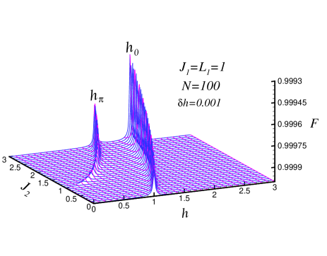
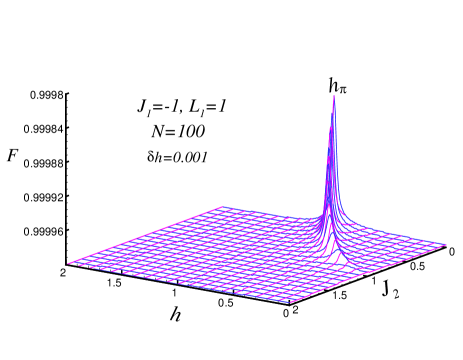
Figure 1: (Color online) Three-dimension of the ground state fidelity of quantum compass model in a transverse field as a function of magnetic field $h$ and Hamiltonian parameter $J_{2}$. The parameters set as (a) $J_{1}=L_{1}=1$, $L_{2}=0$, $N=100$ and $\delta h=0.001$, (b) $J_{1}=-1$, $L_{1}=1$ $L_{2}=0$, $N=100$ and $\delta h=0.001$.

III Fidelity and phase diagram

The phase diagram can be examined by considering the fidelity and fidelity susceptibility introduced in Ref. Zanardi . As mentioned in introduction, the fidelity of ground state is defined by the overlap between the two ground state wave functions at different parameter values and is defined as

$$F(h,\delta h)=|\langle\psi_{0}(h)|\psi_{0}(h+\delta h)\rangle|,$$ (11)

where $|\psi_{0}(h)\rangle$ is a ground state wave function of the many-body Hamiltonian describing the system exposed to an external magnetic field $h$, while $\delta h$ is a small deviation from $h$. The main idea is that near a QPT point there is a sharp enhancement in the degree of distinguishability between two ground states, corresponding to different values of the parameter space which defines the Hamiltonian. This distinguishability can be determined by the fidelity, which for pure states simplify to the amplitude of inner product or overlap. The behavior can be ascribed to a sudden change in the structure of the ground state of the system across the quantum phase transition. Therefore, one expects that fidelity has a minimum at the critical point and it should contain all the information that describes QPTs and topological order. The drop of fidelity specify not only the position of the critical point, but also universal information about the transition given by the critical exponent $\nu$ which is the correlation length exponent associated with the QCPs Zanardi . The response of the fidelity after an infinitesimal change of the external parameter up to second order reads

$$F(h,\delta h)=1-\frac{\delta h^{2}}{2}\chi_{F},$$

where the fidelity susceptibility ($\chi_{F}$) is defined by Venuti ; You2

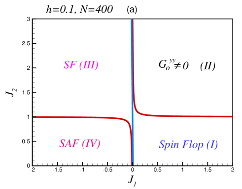
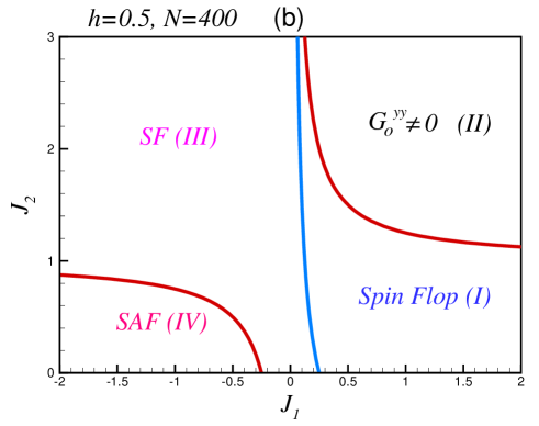
Figure 2: (Color online.) Contour plot of the fidelity of quantum compass model in a transverse field. The parameters set as $L_{1}=1,L_{2}=0,N=400$ and (a) $h=0.1$, (b) $h=0.5$. The light blue line represents $h_{0}=\sqrt{J_{2}+1}$ critical line and $h_{\pi}=\sqrt{J_{2}-1}$ critical line has been shown by the red lines.

$$\chi_{F}=\langle\partial_{h}\psi_{0}(h)|\partial_{h}\psi_{0}(h)\rangle-\langle\partial_{h}\psi_{0}(h)|\psi_{0}(h)\rangle\langle\psi_{0}(h)|\partial_{h}\psi_{0}(h)\rangle.$$ (12)

If there exist more than one external parameter, this result could be generalized to the so-called quantum geometric tensor Zanardi ; Venuti ; Hamma ; Jafari6 .

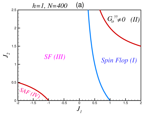
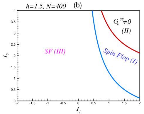
Figure 3: (Color online.) Contour plot of the fidelity of quantum compass model in a transverse field. The parameters set as $L_{1}=1,L_{2}=0,N=400$ and (a) $h=1$, (b) $h=1.5$. $h_{0}=\sqrt{J_{2}+1}$ and $h_{\pi}=\sqrt{J_{2}-1}$ critical lines have been shown by the light blue and the red lines respectively.

The fidelity of this model has been calculated using Eqs. (10) and (11). Three-dimensional panorama of the ground sate fidelity of the model has been depicted in Figs. 1 (a), (b) versus the magnetic field and $J_{2}$ for $J_{1}=1$ and $J_{1}=-1$, where we have set $N=100$ and $\delta h=0.001$. Obviously, there is a sudden drop in the ground state fidelity at the QPTs lines.

In Fig. 1 (a), one observes that the transition lines $h_{0}=\sqrt{J_{2}+1}$ and $h_{\pi}=\sqrt{J_{2}-1}$ are characterized by two assumed lines on the minimum parts of the fidelity surface. However, in Fig. 1 (b) the minimum line on the fidelity surface defined by $h_{\pi}=\sqrt{J_{2}-1}$ clearly indicates a second order phase transition. By computing the fidelity of the one-dimensional extended quantum compass model in a transverse filed, we find the expected critical lines that we already discussed in the context of the exact solution and we illustrate the phase diagram of this model in Figs. 2 (a), (b), 3 (a), (b). In Ref. Jafari3 the phase diagram of this model has been investigated by use of the gap analysis and universality of derivative of the correlation functions. As previously mentioned, the fidelity and fidelity susceptibility of the ground state properties could reflect different zero-temperature regions. This model is always gapful except at the critical surfaces where the energy gap disappears. There are four gapped phases in the exchange couplings’ space:

• Region (I) $J_{1}>0,~{}0<J_{2}<J^{c}_{2}(J_{1},h)$: In this region for $h<h_{0}$ the ground state is in the spin-flop phase (Figs. (2) and (3)).

• Region (II) $J_{1}>0,~{}J_{2}>J^{c}_{2}(J_{1},h)$: In this case there is antiparallel ordering of spin $y$ component on odd bonds ($G_{o}^{yy}\neq 0$)Eriksson ; Mahdavifar ; Jafari3 for $h<h_{\pi}$. In this region tuning $J_{2}$ forces the system go into a spin-flop phase (region (I)).

• Region (III) $J_{1}<|J^{c}_{1}(J_{2},h)|$, $J_{2}>J^{c}_{2}(J_{1},h)$: In this region the ground state is the ferromagnetically polarized state (Saturate Ferromagnetic) along the magnetic field (SF). (Figs. (2) and (3)).

• Region (IV) $J_{1}<0,~{}J_{2}<J^{c}_{2}(J_{1},h)$: In this region the ground state is in the strip antiferromagnetic (SAF) phase for $h<h_{\pi}$.

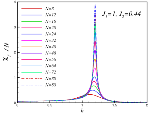
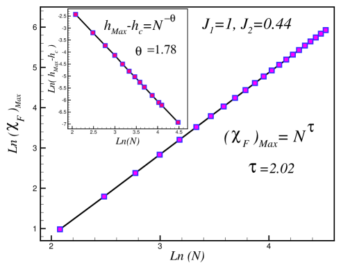
Figure 4: (Color online) (a) Fidelity susceptibility per particle of quantum compass model in a transverse field as a functions of h for various system size for $J_{1}=1,J_{2}=0.44$. (b) Scaling of the maximum of $\chi_{F}$ in terms of system size ($N$). Inset: Scaling of the position ($h_{Max}$) of $\chi_{F}$ for different-length chains where $h_{Max}$ is the position of maximum in Fig.4 (a).

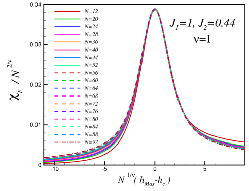
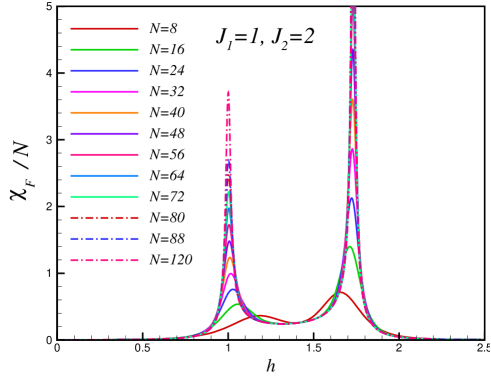
Figure 5: (Color online) (a) The finite-size scaling analysis for the case of logarithmic divergence around the maximum point ($h_{Max}$) for $J_{1}=1,J_{2}=0.44$. The fidelity susceptibility, considered as a function of system size and couplings, collapses on a single curve for different lattice sizes. (b) Fidelity susceptibility of the model as a function of h for different system sizes for $J_{1}=1,J_{2}=2$.

Table 1: The critical exponents $\theta$, $\tau$, $\nu$. The scaling behavior of the susceptibility in the vicinity of the critical points.

$Exchange~{}couplings$	$Critical~{}points$	$\theta$	$\tau$	$\nu$
$J_{1}=1,J_{2}=0.44$	$h_{c}=h_{0}=1.2$	$1.78$	$2.02$	$1.00$
$J_{1}=1,J_{2}=2$	$h_{c_{1}}=h_{\pi}=1.0$	$1.90$	$1.97$	$1.00$
$J_{1}=1,J_{2}=2$	$h_{c_{2}}=h_{0}=\sqrt{3}$	$1.90$	$2.01$	$0.985$
$J_{1}=-1,J_{2}=0.51$	$h_{c}=h_{\pi}=0.7$	$2.70$	$1.93$	$1.01$

IV Universality and scaling of fidelity susceptibility

It is expected that the fidelity susceptibility ($\chi_{F}$) probes the QPTs. Then it will be helpful to study the universality and scaling behavior of $\chi_{F}$ to better understand the properties of the fidelity, and the relation between fidelity and quantum criticality. In this section we investigate the scaling behavior of the fidelity susceptibility by the finite size scaling approach. In Fig. (4) (a) the two dimensional plot of the fidelity susceptibility per particle ($\chi_{F}/N$) has been shown versus the magnetic field for different system sizes for $J_{1}=1,J_{2}=0.44$.

Although there is no real divergence for finite lattice size, but the curves exhibit marked anomalies with height of peak increasing with the system size and in thermodynamics limit $\chi_{F}/N$ diverges as the critical point is touched. More information can be obtained when the maximum values of each plot and their positions are examined. As it manifests the divergences of $\chi_{F}$ occurs at $h_{c}=1.2$ where exactly correspond to the critical point that has been obtained using the energy gap analysis ($h_{c}=h_{0}=\sqrt{1.44}$). Our investigation manifest the scaling behavior of $\chi_{F}$ at the maximum point versus $N$. In this way we have plotted the scaling behavior of $\chi_{F}|_{h_{Max}}$ in Fig. 4 (b), which shows a linear behavior of $\ln(\chi_{F}|_{h_{Max}})$ versus $\ln(N)$ with the exponent $\tau\simeq 2.02\pm 0.01$.

A more detailed analysis shows that the position of the maximum point ($h_{Max}$) of $\chi_{F}$ tends toward the critical point like $h_{Max}=h_{c}+N^{-\theta}$ ($\theta=1.78\pm 0.01$) which has been plotted in the inset of Fig. 4 (b).

To study the scaling behavior of fidelity susceptibility around the critical points, we perform finite-scaling analysis, since the maximum value of $\chi_{F}$ scales logarithmically. Then, by choosing a proper scaling function and taking into account the distance of the maximum of $\chi_{F}$ from the critical point, it is possible to make all the data for the value of $\chi_{F}/N^{2/\nu}$ as a function of $N^{1/\nu}(h_{Max}-h_{c})$ for different $N$ collapse onto a single curve. The analysis of the finite-size scaling is shown in Fig. 5 (a) for several typical lattice sizes. It is clear that the different curves which correspond to various system sizes collapse to a single universal curve as expected from the finite size scaling ansatz. Our result shows that $\nu=1$ exactly corresponds to the correlation length exponent of Ising model in a transverse field ($\nu=1$).

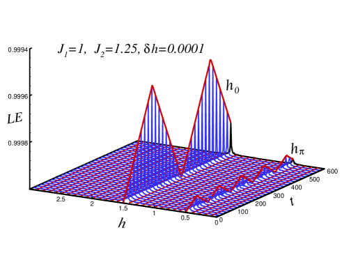
Figure 6: (Color online) Three-dimension of the Loschmidt echo as a functions of magnetic field and time, where the Hamiltonian parameters set as $J_{1}=1,J_{2}=1.25,L_{1}=1,L_{2}=0$ for $N=400$ and $\delta h=0.0001$.

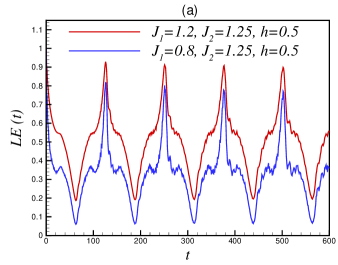
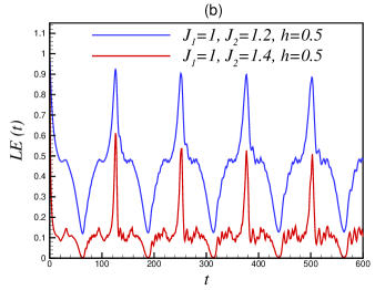
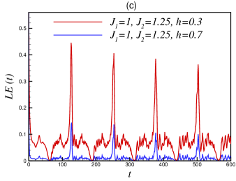
Figure 7: (Color online.) Variation of ground state LE versus the time $t$ to the critical point $J_{1}=1,J_{2}=1.25,L_{1}=1,L_{2}=0,h=0.5$ with $N=400$, starting from different values of the coupling constants and magnetic field (a) $J_{1}=0.8$, $J_{1}=1.2$, (b) $J_{2}=1.2$, $J_{2}=1.4$, (c) $h=0.3$ and $h=0.7$.

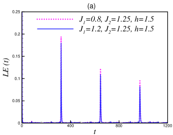
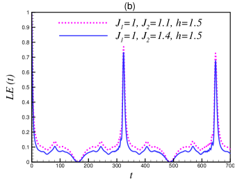
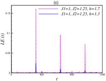
Figure 8: (Color online.) The LE for the quenched quantum compass model to the critical point $J_{1}=1,J_{2}=1.25,L_{1}=1,L_{2}=0,h=1.5$ with $N=400$, starting from different values of parameters (a) $J_{1}=0.8$ and $J_{1}=1.2$, (b) $J_{2}=1.1$ and $J_{2}=1.4$, (c) $h=1.3$ and $h=1.7$.

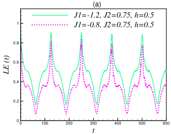
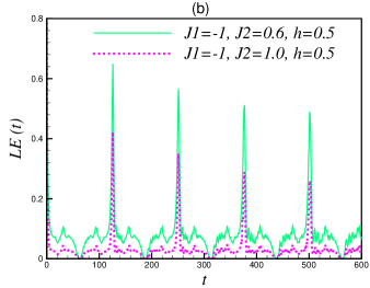
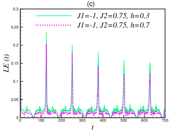
Figure 9: (Color online.) The LE starting from the SAF and SF phases respectively quenched to the critical point $J_{1}=-1,J_{2}=0.75,L_{1}=1,L_{2}=0,h=0.5$ with $N=400$, (a) $J_{1}=-1.2$ and $J_{1}=-0.8$, (b) $J_{2}=0.6$ and $J_{2}=1$, (c) $h=0.3$ and $h=0.7$.

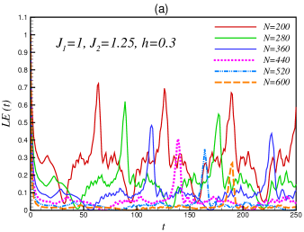
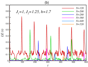
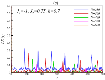
Figure 10: (Color online.) The LE starting from the different phases to the critical points (a) $J_{1}=1,J_{2}=1.25,L_{1}=1,L_{2}=0,h=0.5$, (b) $J_{1}=1,J_{2}=1.25,h=1.5$, (c) $J_{1}=-1,J_{2}=0.75,h=0.5$, for different system sizes.

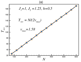
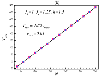
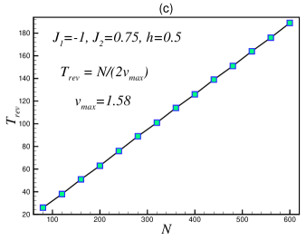
Figure 11: (Color online.) The scaling behavior of the first revival time $T_{rev}$ for different-length chains for a quenches at the different types of critical points (a) $J_{1}=1,J_{2}=1.25,h=0.5$, (b) $J_{1}=1,J_{2}=1.25,L_{1}=1,L_{2}=0,h=1.5$, (c) $J_{1}=-1,J_{2}=0.75,h=0.5$ .

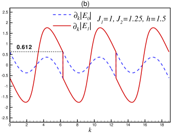
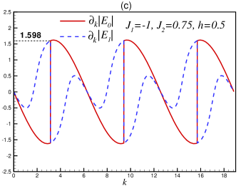
Figure 12: (Color online.) The first derivative of ground state ($E_{0}$) and excited state ($E_{1}$) with respect to the momentum $k$ for quenches at the different critical points (a) $J_{1}=1,J_{2}=1.25,L_{1}=1,L_{2}=0,h=0.5$, (b) $J_{1}=1,J_{2}=1.25,h=1.5$, (c) $J_{1}=-1,J_{2}=0.75,h=0.5$ $h=0.1$, (b) $h=0.5$.

We have plotted $\chi_{F}/N$ for $J_{1}=1$ and $J_{2}=2$ versus $h$ in Fig. 5 (b) for different lattice sizes which shows the singular behavior as the size of the system becomes large. As it manifests the divergences of $\chi_{F}$ occurs at $h_{c_{1}}=1$ and $h_{c_{2}}=\sqrt{3}$. The similar analysis shows the scaling behavior of the position of the first and second maximum point ($h_{Max_{1}},h_{Max_{2}}$) of $\chi_{F}$ tends toward the critical point like $h_{Max_{i}}=h_{c_{i}}+N^{-\theta_{i}}$ ($i=1,2$) and results are presented in Table. (I). Moreover, our results show a linear behavior of $\chi_{F}|_{h_{Max_{i}}}$ versus $\ln(N)$ with the exponent $\tau_{i}$ (see Table I). We illustrate the finite-size scaling behaviors of $\chi_{F}$ around its maximum points. It shows that the fidelity susceptibility can be approximately collapsed to a single curve. These results show that all the key ingredients of the finite-size scaling are present in these cases too. In these cases scaling is fulfilled with the critical exponent $\nu=1$ (see Table. (I)), in agreement with the previous results and the universality hypothesis. The behavior of the fidelity susceptibility has been also investigated in other regions. Our calculations show that the non-analytic and scaling behavior of fidelity susceptibility are the same as the former results with the same finite size scaling (see Table I). It would be worth to mention that the defect density $n_{ex}(h)$ can be related to the fidelity susceptibility $\chi_{F}$ as $n_{ex}=(1/L^{d})h\chi_{F}(h)$, where $L$ is the linear dimension of a $d$-dimensional quantum system. The defect density can be defined for any Hamiltonian system, for a sudden quench close to a quantum critical point Patel . In a sudden quench, when a parameter $h$ in the Hamiltonian of the system is changed suddenly, the wave function of the system does not have sufficient time to evolve. If the system is initially prepared in the ground state for the initial value of the driving parameter, it can not be in the ground state of the final Hamiltonian. Consequently, there are defects in the final state and its scaling follows from the scaling of fidelity susceptibility.

V Quench dynamics and Loschmidt echo

Studying the quench dynamics of the systems can be done in several methods. One of the possible scenarios is Kibble-Zurek mechanism Zurek which estimates the functional dependence of the density of defects on the quenching rate in a system crossing a quantum critical point. Moreover, the Landau-Zener formula Suzuki turns out to be very valuable in investigating the transition probability to the excited state of a two-level systems when a parameter in the Hamiltonian is changed at a slow and uniform rate. Another formalism which has been applied in this section to investigate the time evolution of the ground state after a critical quantum quench is Loschmidt echo. It should be mention that, although the Landau-Zener formalism is a powerful tool to study the quench dynamics of systems, it is not possible to deal with the Hamiltonian of the model Eq. (II) as a two-level system.

As has been mentioned in introduction, a quantum quench is a sudden change in the Hamiltonian of the system. The quantum system is originally prepared in the ground state $|\psi_{0}\rangle$ of $H(h^{(1)})$, and at time $t=0$ the parameters are switched to different values $h^{(2)}$. The system then evolves unitarily with the quench Hamiltonian $H(h^{(2)})$ according to $|\psi_{0}(t)\rangle=U(t)|\psi_{0}\rangle$, where $U(t)=\exp(-iH(h^{(2)})t)$. An important quantity describing the time evolution is the Loschmidt echo (LE) defined as

$$LE(h^{(1)},h^{(2)},t)=|\langle\psi_{0}(h^{(1)})|U(t)|\psi_{0}(h^{(1)})\rangle|^{2},$$ (13)

which gives a measure of the distance between the time evolved state $|\psi_{0}(t)\rangle$ and the initial state $|\psi_{0}\rangle$. High values of the LE mean that the system is approaching the initial state ($LE(t=0)=1$). The LE typically decays exponentially in a short time $T_{rel}$ (relaxation time) from 1 to its average value, around which it oscillates. Revivals are also visible in the LE as deviations from the average value. The revivals have been defined as a time instances ($T_{rev}$) at which the signal $LE(t)$ differs from the average value. The structure of these revivals could be greatly affected by criticality Quan . Since the model is exactly solvable and the whole spectrum and the eigenstate of the model has been obtained, this leads to an exact expression for the LE, and the revival times can be extracted by inspecting its time dependence. To obtain the analytical expression for LE, we should express the old ground state $|\psi_{0}(h^{(1)})\rangle$ in terms of the eigenstates of the quench Hamiltonian $H(h^{(2)})$. The time evolution in the EQC model in a transverse field after a quantum quench is given by:

$$|\psi_{0}(t)\rangle=\frac{1}{\sqrt{N_{0}(h^{(1)})}}\Big{[}\sum_{m=0}^{7}\frac{e^{-\imath E_{m}(h^{(2)})t}}{\sqrt{N_{m}(h^{(2)})}}\sum_{j=1}^{8}v^{(0)}_{j}(h^{(1)})(v^{(m)}_{j}(h^{(2)}))^{\ast}|\psi_{m}(h^{(2)})\rangle\Big{]},$$

where $N_{m}=\sqrt{|\langle\psi_{m}|\psi_{m}\rangle|},~{}(m=0,\cdots,8)$, and the $LE$ is thus

$$LE(h^{(1)},h^{(1)},t)=\Big{|}\frac{1}{N_{0}(h^{(1)})}\Big{[}\sum_{m=0}^{7}\frac{e^{-\imath E_{m}(h^{(2)})t}}{N_{m}(h^{(2)})}\Big{(}\sum_{j=1}^{8}v^{(0)}_{j}(h^{(1)})(v^{(m)}_{j}(h^{(2)}))^{\ast}\Big{)}\Big{(}\sum_{n=1}^{8}(v^{(0)}_{j}(h^{(1)}))^{\ast}(v^{(m)}_{n}(h^{(2)}))\Big{)}\Big{]}\Big{|}^{2}$$

In the following, the detailed analysis of the LE has been shown for different types of quenches. Three-dimensional panorama of the LE has been plotted as a functions of a transverse field and $t$ in Fig. 6 for $J_{1}=1$, $J_{2}=1.25$ and system size set as $N=100$. As one can see, LE experiences a sharp decay around the critical points $h_{\pi}=0.5$ and $h_{0}=1.5$ which exactly correspond to the critical points that have been obtained using the fidelity and gap analysis $h_{\pi}=\sqrt{(J_{1}+L_{2})(J_{2}-L_{1})},~{}h_{0}=\sqrt{(J_{1}+L_{2})(J_{2}+L_{1})}$. As it is clear, the structure of revivals are different at the critical points and $T_{rev}(h_{0})/T_{rev}(h_{\pi})\simeq 2.5$.

Consider the critical pint $J_{1}=1,J_{2}=1.25,h=0.5$. As we see in Fig. 2 (b), this point lies between two different phases. Increasing (decreasing) $J_{1}$ and $J_{2}$ (magnetic field $h$) forces the system into the antiparallel ordering of the $y$ spin component on even bonds phase and decreasing (increasing) $J_{1}$ and $J_{2}$ (magnetic field $h$) drive the model to the spin-flop phase. In Fig. 7 LE has been plotted for a different types of quenches. For this critical point the behavior of the LE does not depend on which phase the system is prepared in qualitatively, and $T_{rev}$ is the same for all the quenches.

In Fig. 8 the system is quenched from different ground states corresponding to different phases (saturate ferromagnetic phase and spin-flop phase) to the critical point $J_{1}=1,J_{2}=1.25,h=1.5$. The numerical simulations show that the details of the evolution are somewhat different, but the structure of the revivals is the same for all the quenches, and it oscillates around a relatively high mean value in Fig. 8 (b) in compare with those one in Figs. 8 (a) and 8 (c). The behavior of the LE after a quench of $J_{1}$ and magnetic field (Figs. 8 (a) (c)) are similar to the one obtained for critical quenches in the XY model Happola .

We also quench to the critical point $J_{1}=-1,J_{2}=0.75,h=0.5$ which lies between SAF phase and SF phase (Fig. (9)). In this case, the details of the LE evolution are the same too, and the only difference is their oscillations around a different mean values. These indicate the universality of the revival structure in which the initial state and the size of the quench are unimportant. The question which is relevant in the measurement process is how the revivals time ($T_{rev}$) can be derived in the LE? We can address this question for the class of quasifree Fermi systems to Refs. Happola ; Montes in which the phenomenon of the revivals after a quantum quench is construed as a recombination of the fastest quasiparticles in the system. Specifically, the speed of the fastest excitations in the system is upper bounded by the Lieb-Robinson speed and this upper bound gives a lower bound to the revival time Montes . On the other hand, the most distinct revivals are given by the steady values of the group velocity $v_{g}(k)=|\frac{\partial(E_{k}^{q}+E_{k}^{p})}{\partial k}|=|\frac{\partial E_{0}}{\partial k}|$ Happola and in this scenario the first revival is the one corresponding to the maximum group velocity ($v_{max}=\max_{k}v_{g}(k)$) and the revival time scale could be given by the following estimate

$$T_{rev}=\frac{N}{2v_{max}}.$$ (14)

To investigate the revival times in LE of the extended quantum compass model in a transverse field, we have plotted the LE for various system sizes in Fig. 10 for different types of quenches. It is easy to see that increasing the length of the chain decreases the oscillation of the LE and the height of first revival decreases gradually and, finally, vanishes as $N\rightarrow\infty$. Examining the details shows the scaling behavior of first revival time $T_{rev}$ versus $N$. This is plotted in Fig. 11, which shows the linear behavior of $T_{rev}$ versus $N$. The scaling behavior is

$$T_{rev}=KN^{\delta},$$ (15)

with exponent $\delta=1$.

A similar analysis can be carried out to obtain the $K$ coefficient. Our calculations show that $K=\frac{1}{2v_{max}}$ where $v_{max}$ are given by following estimate

$$v_{max}=\min(|\frac{\partial(E_{k}^{q}\pm E_{k}^{p})}{\partial k}|_{max})=\min(|\frac{\partial E_{0}}{\partial k}|_{max},|\frac{\partial E_{1}}{\partial k}|_{max})$$

In Fig. 11 the first derivative of the ground state $E_{0}$ and excited state $E_{1}$ with respect to the momentum $k$ has been depicted for different critical points. The numerical calculations show that $v_{max}=\min(|\frac{\partial E_{0}}{\partial k}|_{max},|\frac{\partial E_{1}}{\partial k}|_{max})$ and the revival time shows the universality and scaling around the quantum critical points consistent with those predicted by Eq. (15) and $T_{rev}(h_{0})/T_{rev}(h_{\pi})=v_{max}(h_{\pi})/v_{max}(h_{0})=2.61$ which consistent with those obtained in Fig. 6. A surprising result occurs in the critical surfaces which are the boundaries between the spin-flop (I) and the saturated ferromagnetic (III) phases and between the strip antiferromagnetic (IV) and the saturated ferromagnetic (III) phases which correspond to $h_{\pi}=\sqrt{(J_{1}+L_{2})(J_{2}-L_{1})}$. In this critical magnetic field, the revival time of the LE is inversely proportional to the the maximum group velocity of the excited state quasiparticles, while in $h_{0}=\sqrt{(J_{1}+L_{2})(J_{2}+L_{1})}$ critical field the revival time is proportional to the inverse of the maximum group velocity of the ground state quasiparticles. It should be pointed out that the regions of phase space with a different Lieb-Robinson speed do not correspond to different quantum phases. Quantum phase transition happens in the ground state at a singular point of the phase space, whereas the Lieb-Robinson speed is the maximum speed of any signal in any state and not just small excitations over the ground state Schwarz .

VI Summary and conclusions

In this work we have studied the ground state fidelity, fidelity susceptibility, and quench dynamics of the one-dimensional extended quantum compass model (EQCM) in a transverse field. We use the Jordan-Wigner transformation to construct an explicit analytic expressions of the ground state fidelity and Loschmidt echo (LE) of this model. We show how the fidelity susceptibility and LE could detect the quantum phase transitions in the inhomogeneous system. Moreover, we have investigated the universality and scaling properties of fidelity susceptibility and revival time. The results show that the fidelity susceptibility exhibits beautiful scaling law close to the critical points with exponent $\nu=1$ exactly corresponds to the correlation length exponent of the Ising model in a transverse field.

We show that the LE exhibits a universal structure of revivals that is independent of the initial state and the size of the quench. The information travels through the spin system via wave packets of quasiparticles, and the first revival appears when the wave packets propagates with the minimum of the group velocities of ground state and excited state. This interpretation explain the universality of the revival structure since group velocities only depends on the dispersion relation of the quasiparticles related to the ground state and excited state of the quench Hamiltonian. Depending on the critical surfaces, the structure of the revivals after critical quantum quenches represents two different equilibration dynamics, whereas examination of the fidelity susceptibility shows the same correlation length exponent for all critical points.

VII Appendix

VII.1 Unitary Transformation

The unitary transformation matrix $U$ which can transform the Hamiltonian Eq. (1)into a diagonal form, has the following form

$$U=\left(\begin{array}[]{cccc}U_{1,E_{k}^{q}}&U_{2,E_{k}^{q}}&U_{3,E_{k}^{q}}&1\\ U_{1,-E_{k}^{q}}&U_{2,-E_{k}^{q}}&U_{3,-E_{k}^{q}}&1\\ U_{1,E_{k}^{p}}&U_{2,E_{k}^{p}}&U_{3,E_{k}^{p}}&1\\ U_{1,-E_{k}^{p}}&U_{2,-E_{k}^{p}}&U_{3,-E_{k}^{p}}&1\\ \end{array}\right),$$ (20)

where

$$U_{1,\pm E_{k}^{\alpha}} = \frac{\frac{2h\pm E_{k}^{\alpha}}{J^{\ast}}-\frac{L^{\ast}}{J^{\ast}}\Big{[}\frac{L^{\ast}(2h\pm E_{k}^{\alpha})}{{L^{\ast}}^{2}-{J^{\ast}}^{2}}-J^{\ast}\Big{(}(2h\mp E_{k}^{\alpha})\Big{(}L({J^{\ast}}^{2}-{L^{\ast}}^{2})-L^{\ast}(2h\pm E_{k}^{\alpha})^{2}\Big{)}\Big{)}\Big{]}}{\Big{[}{L^{\ast}}^{2}-{J^{\ast}}^{2}\Big{]}\Big{[}J^{\ast}(\gamma a-|L|^{2})-J{L^{\ast}}^{2}\Big{]}},$$

$$U_{2,\pm E_{k}^{\alpha}} = \frac{\Big{[}\frac{-L^{\ast}(2h\pm E_{k}^{\alpha})}{{L^{\ast}}^{2}-{J^{\ast}}^{2}}+J^{\ast}\Big{(}(2h\mp E_{k}^{\alpha})\Big{(}L({J^{\ast}}^{2}-{L^{\ast}}^{2})-L^{\ast}(2h\pm E_{k}^{\alpha})^{2}\Big{)}\Big{)}\Big{]}}{\Big{[}{L^{\ast}}^{2}-{J^{\ast}}^{2}\Big{]}\Big{[}J^{\ast}(\gamma a-|L|^{2})-J{L^{\ast}}^{2}\Big{]}},$$

$$U_{3,\pm E_{k}^{\alpha}} = -\frac{\Big{[}L({J^{\ast}}^{2}-{L^{\ast}}^{2})-L^{\ast}(2h\pm E_{k}^{\alpha})^{2}\Big{)}\Big{]}}{\Big{[}J^{\ast}(\gamma a-|L|^{2})-J{L^{\ast}}^{2}\Big{]}},$$

$\alpha=q,p$, $\gamma=1$ for $\alpha=q$ and $\gamma=-1$ for $\alpha=p$.

VII.2 Ground State

By using the unitary transformation the unnormalized eigenvectors and eigenvalues have the following expressions in terms of the coupling constants:

$$|\psi_{m}\rangle=\prod_{k} [ v_{1}^{m}|0\rangle+v_{2}^{m}~{}c_{k}^{{q{\dagger}}}c_{-k}^{{q{\dagger}}}|0\rangle+v_{3}^{m}~{}c_{k}^{{q{\dagger}}}c_{-k}^{{p{\dagger}}}|0\rangle+v_{4}^{m}~{}c_{-k}^{{q{\dagger}}}c_{k}^{{p{\dagger}}}|0\rangle+v_{5}^{m}~{}c_{k}^{{p{\dagger}}}c_{-k}^{{p{\dagger}}}|0\rangle+v_{6}^{m}~{}c_{k}^{{q{\dagger}}}c_{k}^{{p{\dagger}}}|0\rangle$$

$$+ v_{7}^{m}~{}c_{-k}^{{q{\dagger}}}c_{-k}^{{p{\dagger}}}|0\rangle+v_{8}^{m}~{}c_{k}^{{q{\dagger}}}c_{-k}^{{q{\dagger}}}c_{k}^{{p{\dagger}}}c_{-k}^{{p{\dagger}}}|0\rangle],~{}m=0,1,\cdots,7.$$

$$E_{0} = -\sqrt{2}\sqrt{4h^{2}+|J|^{2}+|L|^{2}+C},$$

$$v_{1}^{0} = \frac{64h^{4}-{J^{\ast}}^{2}L^{2}+J^{2}(2{J^{\ast}}^{2}-{L^{\ast}}^{2})+2|J|^{2}C-16E_{0}h^{3}-4h(|J|^{2}-|L|^{2}+C)E_{0}+8h^{2}(3|J|^{2}-2|L|^{2}+2C)}{8h^{2}|J|^{2}+2|J|^{2}C+2|J|^{4}-J^{2}{L^{\ast}}^{2}-{J^{\ast}}^{2}L^{2}},$$

$$v_{2}^{0} = v_{5}^{0}=-\frac{E_{0}(4h-E_{0})(LJ^{\ast}-JL^{\ast})/2}{8h^{2}|J|^{2}+2|J|^{2}C+2|J|^{4}-J^{2}{L^{\ast}}^{2}-{J^{\ast}}^{2}L^{2}},$$

$$v_{3}^{0} = -\frac{(4h-E_{0})(4h^{2}J+{J^{\ast}}(J^{2}-L^{2})+JC)}{8h^{2}|J|^{2}+2|J|^{2}C+2|J|^{4}-J^{2}{L^{\ast}}^{2}-{J^{\ast}}^{2}L^{2}},$$

$$v_{4}^{0} = -\frac{(4h-E_{0})(4h^{2}{J^{\ast}}+J({J^{\ast}}^{2}-{L^{\ast}}^{2})+{J^{\ast}}C)}{8h^{2}|J|^{2}+2|J|^{2}C+2|J|^{4}-J^{2}{L^{\ast}}^{2}-{J^{\ast}}^{2}L^{2}},$$

$$v_{6}^{0} = ~{}v_{7}^{0}=0,~{}v_{8}^{0}=1,$$

$$E_{1} = -\sqrt{2}\sqrt{4h^{2}+|J|^{2}+|L|^{2}-C},$$

$$v_{1}^{1} = \frac{-64h^{4}+{J^{\ast}}^{2}L^{2}-J^{2}(2{J^{\ast}}^{2}-{L^{\ast}}^{2})+2|J|^{2}C+16E_{1}h^{3}+4h(|J|^{2}-|L|^{2}-C)E_{1}-8h^{2}(3|J|^{2}-2|L|^{2}-2C)}{-8h^{2}|J|^{2}+2|J|^{2}C-2|J|^{4}+J^{2}{L^{\ast}}^{2}+{J^{\ast}}^{2}L^{2}},$$

$$v_{2}^{1} = v_{5}^{1}=-\frac{E_{1}(4h-E_{1})(LJ^{\ast}-JL^{\ast})/2}{-8h^{2}|J|^{2}+2|J|^{2}C-2|J|^{4}+J^{2}{L^{\ast}}^{2}+{J^{\ast}}^{2}L^{2}},$$

$$v_{3}^{1} = -\frac{(4h-E_{0})(4h^{2}J+{J^{\ast}}(J^{2}-L^{2})-JC)}{-8h^{2}|J|^{2}+2|J|^{2}C-2|J|^{4}+J^{2}{L^{\ast}}^{2}+{J^{\ast}}^{2}L^{2}},$$

$$v_{4}^{1} = -\frac{(4h-E_{0})(4h^{2}{J^{\ast}}+J({J^{\ast}}^{2}-{L^{\ast}}^{2})-{J^{\ast}}C)}{-8h^{2}|J|^{2}+2|J|^{2}C-2|J|^{4}+J^{2}{L^{\ast}}^{2}+{J^{\ast}}^{2}L^{2}},$$

$$v_{6}^{1} = ~{}v_{7}^{1}=0,~{}v_{8}^{1}=1,$$

$$E_{2}=0,~{}v_{2}^{1}=v_{2}^{3}=v_{2}^{4}=v_{2}^{6}=v_{2}^{7}=v_{2}^{8}=0,v_{2}^{2}=-v_{2}^{5}=-1,$$

$$E_{3}=0,~{}v_{3}^{1}=v_{3}^{2}=v_{3}^{3}=v_{3}^{4}=v_{3}^{5}=v_{3}^{7}=v_{3}^{8}=0,v_{3}^{6}=1,$$

$$E_{4}=0,~{}v_{4}^{1}=v_{4}^{2}=v_{4}^{3}=v_{4}^{4}=v_{4}^{5}=v_{4}^{6}=v_{4}^{8}=0,v_{4}^{7}=1,$$

$$E_{5}=0,~{}v_{5}^{2} = v_{5}^{5}=v_{5}^{6}=v_{5}^{7}=0,~{}v_{5}^{1}=-v_{5}^{8}=-1,$$

$$v_{5}^{3} = \frac{4hL}{L{J^{\ast}}+J{L^{\ast}}},~{}v_{5}^{4}=\frac{4h{L^{\ast}}}{L{J^{\ast}}+J{L^{\ast}}},$$

$$E_{6} = \sqrt{2}\sqrt{4h^{2}+|J|^{2}+|L|^{2}-C},$$

$$v_{1}^{6} = \frac{-64h^{4}+{J^{\ast}}^{2}L^{2}-J^{2}(2{J^{\ast}}^{2}-{L^{\ast}}^{2})+2|J|^{2}C+16E_{6}h^{3}+4h(|J|^{2}-|L|^{2}-C)E_{6}-8h^{2}(3|J|^{2}-2|L|^{2}-2C)}{-8h^{2}|J|^{2}+2|J|^{2}C-2|J|^{4}+J^{2}{L^{\ast}}^{2}+{J^{\ast}}^{2}L^{2}},$$

$$v_{2}^{6} = v_{5}^{6}=-\frac{E_{6}(4h-E_{6})(LJ^{\ast}-JL^{\ast})/2}{-8h^{2}|J|^{2}+2|J|^{2}C-2|J|^{4}+J^{2}{L^{\ast}}^{2}+{J^{\ast}}^{2}L^{2}},$$

$$v_{3}^{6} = \frac{(4h-E_{6})(4h^{2}J+{J^{\ast}}(J^{2}-L^{2})-JC)}{-8h^{2}|J|^{2}+2|J|^{2}C-2|J|^{4}+J^{2}{L^{\ast}}^{2}+{J^{\ast}}^{2}L^{2}},$$

$$v_{4}^{6} = \frac{(4h-E_{6})(4h^{2}{J^{\ast}}+J({J^{\ast}}^{2}-{L^{\ast}}^{2})-{J^{\ast}}C)}{-8h^{2}|J|^{2}+2|J|^{2}C-2|J|^{4}+J^{2}{L^{\ast}}^{2}+{J^{\ast}}^{2}L^{2}},$$

$$v_{6}^{6} = ~{}v_{7}^{6}=0,~{}v_{8}^{6}=1,$$

$$E_{7} = \sqrt{2}\sqrt{4h^{2}+|J|^{2}+|L|^{2}+C}$$

$$v_{1}^{7} = \frac{64h^{4}-{J^{\ast}}^{2}L^{2}+J^{2}(2{J^{\ast}}^{2}-{L^{\ast}}^{2})+2|J|^{2}C-16E_{7}h^{3}-4h(|J|^{2}-|L|^{2}+C)E_{7}+8h^{2}(3|J|^{2}-2|L|^{2}+2C)}{8h^{2}|J|^{2}+2|J|^{2}C+2|J|^{4}-J^{2}{L^{\ast}}^{2}-{J^{\ast}}^{2}L^{2}},$$

$$v_{2}^{7} = v_{5}^{7}=-\frac{E_{7}(4h-E_{7})(LJ^{\ast}-JL^{\ast})/2}{-8h^{2}|J|^{2}-2|J|^{2}C-2|J|^{4}+J^{2}{L^{\ast}}^{2}+{J^{\ast}}^{2}L^{2}},$$

$$v_{3}^{7} = -\frac{(4h-E_{7})(4h^{2}J+{J^{\ast}}(J^{2}-L^{2})+JC)}{8h^{2}|J|^{2}+2|J|^{2}C+2|J|^{4}-J^{2}{L^{\ast}}^{2}-{J^{\ast}}^{2}L^{2}},$$

$$v_{4}^{7} = -\frac{(4h-E_{7})(4h^{2}{J^{\ast}}+J({J^{\ast}}^{2}-{L^{\ast}}^{2})+{J^{\ast}}C)}{8h^{2}|J|^{2}+2|J|^{2}C+2|J|^{4}-J^{2}{L^{\ast}}^{2}-{J^{\ast}}^{2}L^{2}},$$

$$v_{6}^{7} = ~{}v_{7}^{7}=0,~{}v_{8}^{7}=1,$$

in which $C=\sqrt{a^{2}-b}$.

References

References

- (1) A. Osterloh, Luigi Amico, G. Falci, and Rosario Fazio, Nature (London) 416, 608 (2002).
- (2) G. Vidal, J. I. Latorre, E. Rico, and A. Kitaev, Phys. Rev. Lett. 90, 227902 (2003).
- (3) T. J. Osborne, M. A. Nielsen, Phys. Rev. A. 66, 032110 (2002); G. Vidal, J. I. Latorre, E. Rico, and A. Kitaev, Phys. Rev. Lett. 90, 227902 (2003); Y. Chen, P. Zanardi, Z. D. Wang, F. C. Zhang, New J. Phys. 8, 97 (2006); L. A. Wu, M. S. Sarandy, D. A. Lidar, Phys. Rev. Lett. 93, 250404 (2004).
- (4) M. Kargarian, R. Jafari and A. Langari, Phys. Rev. A 76, 060304(R) (2007).
- (5) M. Kargarian, R. Jafari, and A. Langari, Phys. Rev. A 77, 032346 (2008).
- (6) R. Jafari, M. Kargarian, A. Langari, and M. Siahatgar, Phys. Rev. B 78, 214414 (2008).
- (7) M. Kargarian, R. Jafari and A. Langari, Phys. Rev. A 79, 042319 (2009).
- (8) R. Jafari, Phys. Rev. A 82, 052317 (2010).
- (9) A. Langari, and A. T. Rezakhani, New J. Phys. 14 053014 (2012); N. Amiri, and A. Langari, Phys. Status Solidi B. 250, 537 (2013).
- (10) R. Jafari and A. Langari, Int. J. Quantum Inf. 9 (04), 1057, (2011).
- (11) E. Mehran, S. Mahdavifar, R. Jafari, Phys. Rev. A. 89, 049903, (2014).
- (12) R. Jafari, S. Mahdavifar, Prog. Theor. Exp. Phys. 4, 043I02 (2014).
- (13) P. Zanardi, P Giorda, and M. Cozzini, Phys. Rev. Lett. 99, 100603 (2007); P. Zanardi and N. Paunkovic, Phys. Rev. E 74, 031123 (2006).
- (14) M. Greiner, O. Mandel, T. W. Hänsch, and I. Bloch, Nature (London) 415, 39 (2002).
- (15) D. Jaksch, C. Bruder, J. I. Cirac, C. W. Gardiner, and P. Zoller, Phys. Rev. Lett. 81, 3108 (1998).
- (16) T. Stöferle, H. Moritz, C. Schori, M. Kühl, and T. Esslinger, Phys. Rev. Lett. 92, 130403 (2004).
- (17) Quantum Quenching, Annealing and Computation, edited by A. K. Chandra, A. Das, and B. K. Chakrabarti (Springer, Heidelberg, 2010).
- (18) T. Gorin, T. Prosen, T. H. Seligman, and M. Znidaric, Phys. Rep. 435, 33 (2006).
- (19) Ph. Jacquod and C. Petitjean, Adv. Phys. 58, 67 (2009).
- (20) L. Campos Venuti, N. T. Jacobson, S. Santra, and P. Zanardi, Phys. Rev. Lett. 107, 010403 (2011).
- (21) H. T. Quan, Z. Song, X. F. Liu, P. Zanardi, and C. P. Sun, Phys. Rev. Lett. 96, 140604 (2006).
- (22) S. Montes, and A. Hamma, Phys. Rev. E. 86, 021101 (2012).
- (23) E. Eriksson and H. Johannesson, Phys. Rev. B 79, 224424 (2009).
- (24) S. Mahdavifar, Eur. Phys. J. B 77, 77 (2010).
- (25) M. Motamedifar, S. Mahdavifar, and S. F. Shayesteh, Eur. Phys. J. B 83, 181 (2011).
- (26) R. Jafari, Phys. Rev. B 84, 035112 (2011).
- (27) R. Jafari, Eur. Phys. J. B 85, 167 (2012).
- (28) W. L. You, Eur. Phys. J. B 85, 83 (2012).
- (29) G.H. Liu, W. Li, and W. L. You, Eur. Phys. J. B 85, 168 (2012).
- (30) M. Motamedifar, S. Nemati, S. Mahdavifar, and S. F. Shayesteh, Phys. Scr. 88, 015003 (2013).
- (31) J. Häppölä, G. B. Halász, and A. Hamma, Phys. Rev. A 85, 032114 (2012).
- (32) G. Vidal, Phys. Rev. Lett. 98, 070201 (2007).
- (33) E. Lieb, T. Schultz, and D. Mattis, Ann. Phys. (N.Y.) 16, 407 (1961); E. Barouch and B. M. McCoy, Phys. Rev. A 3, 786 (1971); J. B. Kogut, Rev. Mod. Phys. 51, 659 (1979); J. E. Bunder and R. H. McKenzie, Phys. Rev. B 60, 344 (1999).
- (34) J. H. H. Perk, H. W. Capel, and M. J. Zuilhof, Physica 81A 319 (1975).
- (35) K. Sengupta, D. Sen, and S. Mondal, Phys. Rev. Lett. 100, 077204 (2008); S. Mondal, D. Sen, and K. Sengupta, Phys. Rev. B 78, 045101 (2008).
- (36) Wen-Long You, Ying-Wai Li, and Shi-Jian Gu, Phys. Rev. E 76, 022101 (2007).
- (37) L. Campos Venuti and P. Zanardi, Phys. Rev. Lett. 99, 095701 (2007).
- (38) A. Hamma, e-print: quant-ph/0602091.
- (39) R. Jafari, Phys. Lett. A 377,3279 (2013).
- (40) Aavishkar A. Patel and Amit Dutta, Phys. Rev. B. 86, 174306 (2012).
- (41) W. H. Zurek, U. Dorner, and P. Zoller, Phys. Rev. Lett. 95, 105701 (2005).
- (42) S. Suzuki and M. Okada, in Quantum annealing and related optimization methods edited by A Das and B K Chakrabarti (Springer-Verlag, Berlin, 2005) p. 185.
- (43) I. Prémont-Schwarz, and J. Hnybida, Phys. Rev. A. 81, 062107 (2010).