A closer look at coupled logistic maps at the edge of chaos

Abstract

We focus on a linear chain of $N$ first-neighbor-coupled logistic maps at their edge of chaos in the presence of a common noise. This model, characterised by the coupling strength $\epsilon$ and the noise width $\sigma_{max}$, was recently introduced by Pluchino et al [Phys. Rev. E 87, 022910 (2013)]. They detected, for the time averaged returns with characteristic return time $\tau$, possible connections with $q$-Gaussians, the distributions which optimise, under appropriate constraints, the nonadditive entropy $S_{q}$, basis of nonextensive statistics mechanics. We have here a closer look on this model, and numerically obtain probability distributions which exhibit a slight asymmetry for some parameter values, in variance with simple $q$-Gaussians. Nevertheless, along many decades, the fitting with $q$-Gaussians turns out to be numerically very satisfactory for wide regions of the parameter values, and we illustrate how the index $q$ evolves with $(N,\tau,\epsilon,\sigma_{max})$. It is nevertheless instructive on how careful one must be in such numerical analysis. The overall work shows that physical and/or biological systems that are correctly mimicked by the Pluchino et al model are thermostatistically related to nonextensive statistical mechanics when time-averaged relevant quantities are studied.

I Introduction

Synchronization has long been observed in complex systems and extensively studied in the literature synch1 ; synch2 . In these studies, coupled maps are considered as an important theoretical model for these systems kaneko . Moreover, since many biological systems evolve in noisy environments, it is important to analyse the effect of noise in such coupled maps. Recently, the effect of weak noise on globally coupled chaotic units has been studied for several systems kaneko2 ; kuramoto .

The model that we focus on here is a linear chain of $N$ coupled logistic maps, with periodic boundary conditions, and can be written as

$$x_{t+1}^{i}=(1-\epsilon)f\left(x_{t}^{i}\right)+\frac{\epsilon}{2}\left[f\left(x_{t}^{i-1}\right)+f\left(x_{t}^{i+1}\right)\right]+\sigma(t)$$ (1)

where $\epsilon\in[0,1]$ is the local coupling, and $\sigma(t)$ is an additive random noise uniformly distributed in $[0,\sigma_{max}]$, which fluctuates in time but is equal for all maps. Here, the $i$th logistic map at any time $t$ is given as

$$f\left(x_{t}^{i}\right)=1-\mu\left|x_{t}^{i}\right|^{2}$$ (2)

where $\mu\in[0,2]$ is the map parameter and this function is taken in module 1 with sign in order to fold the iterates of the maps back into the map interval $[-1,1]$ if the noise takes them out of this interval. All elements of the system will be kept at the chaos threshold by fixing the $\mu$ parameter at $\mu_{c}=1.40115518909...\,$.

Very recently, the probability distribution functions (PDFs) of the returns for this model have been investigated numerically by Pluchino et al.Alex2013 and fat-tailed distributions have been reported, which can be fitted by $q$-Gaussians. The physical quantity under investigation, the returns, is a commonly used one in areas such as turbulence turbulence , finance finance ; finance2 , DNA sequences DNA , and earthquake dynamics caruso ; bakar1 ; bakar2 ; ahmet in the literature. It is defined as

$$\Delta d_{t}=d_{t+\tau}-d_{t}$$ (3)

where

$$d_{t}=\frac{1}{N}\sum_{i=1}^{N}\left|x_{t}^{i}-\left<x_{t}^{i}\right>\right|\,\,.$$ (4)

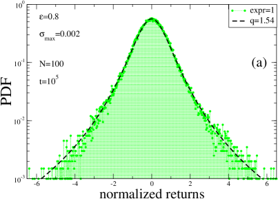
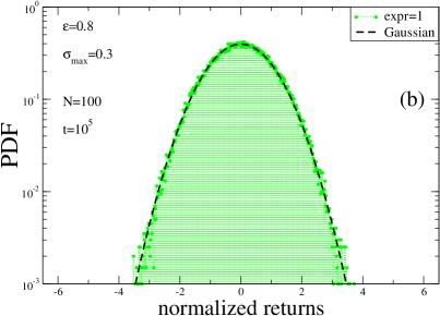
Figure 1: Probability distribution functions of the normalized returns for $N=100$ logistic maps at the edge of chaos with $\tau=32$. The parameter values used here are exactly those of Fig. 3a (case (a)) and of Fig. 3d (case (b)) of Alex2013 . By expr $=1$ we mean that only one experiment has been done in each of these illustrations.

The main result of Alex2013 has been given in Fig. 3 of that paper where the PDFs of the normalized returns (normalized to the standard deviation of the overall sequence) have been plotted for various $\sigma_{max}$ values. We have reproduced here in our Fig. 1 two representative cases, namely, $\sigma_{max}=0.002$ and $\sigma_{max}=0.3$ to be compared with Fig. 3a and Fig. 3d of Alex2013 , respectively. It is evident that the $q$-Gaussian curves with predicted $q$ values are very reasonable for these examples ($q=1.54$ for $\sigma_{max}=0.002$ and $q=1$ for $\sigma_{max}=0.3$). However, the distributions span less than 3 decades since the time series that have been used are relatively short ($t=10^{5}$). Therefore it is interesting to check the behaviour with longer time series in order to span more decades of the PDF. This is what we have done: see Fig. 2, which has been obtained by considering a large number of experiments (250 and 500). This means that the time series analysed are as long as $250\times 10^{5}$ and $500\times 10^{5}$ respectively. As seen clearly from Fig. 2, when one more decade is exhibited for the tails, the departure from the a priori admissible $q$-Gaussians becomes clearly visible.

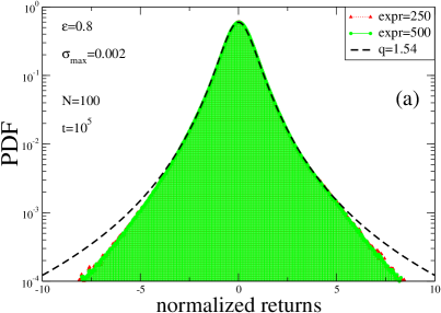
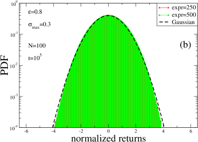
Figure 2: Probability distribution functions of the normalized returns for $N=100$ logistic maps at the edge of chaos with $\tau=32$ for $\sigma_{max}=0.002$ (a) and $\sigma_{max}=0.3$ (b). In order to analyse the tails of the distribution, large number of experiments is used. The size of the time series therefore equals to the number of experiments times the time steps used in each experiment (i.e., expr$\times 10^{5}$).

In addition to this, it is also interesting to check whether these typical numerical PDFs are asymptotic in the sense of the $N\to\infty$ limit. If this is the case, one would expect the PDF curves to remain basically invariant as the size $N$ of the system increases. We have checked it: see two illustrative cases in Fig. 3. It is easily seen that the $N=100$ size cannot be considered as sufficient for the analysis of the asymptotic behaviour, especially for small values of $\sigma_{max}$.

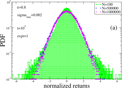
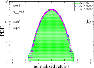
Figure 3: Probability distribution functions of the normalized returns for $N$ logistic maps at the edge of chaos with $\tau=32$ for $N=100$, $N=100000$ and $N=500000$. It is evident that, as $N$ increases, the asymptotic PDFs are attained slowly for small $\sigma_{max}$ values (i.e., case (a)), whereas it is quite quick for larger $\sigma_{max}$ values (i.e., case (b)).

It is therefore clear at this stage that, if we are particularly interested in studying the asymptotic behaviour of PDFs of the normalized returns of this system, both the size $N$ of the system and the length of the time series must be quite large. To further refine numerically the present analysis, we have also studied the same two cases with large enough value for $N$ ($N=500000$ for $\sigma_{max}=0.002$. and $N=200000$ for $\sigma_{max}=0.3$), and with a time series of $100\times 10^{6}$ steps. These conditions are sufficient to observe the behaviour up to almost 6 decades. The results are given in Fig. 4. The strong departure from the $q$-Gaussians with early predicted $q$ values becomes now very obvious. Moreover, a slight but neat asymmetry emerges for small $\sigma_{max}$. In order to fit this kind of behavior, one can use a non-symmetric extension of $q$-Gaussian, namely given by

$$p\propto\left[1-(1-q)(bx^{2}+gx^{3})\right]^{1/(1-q)}\,,$$ (5)

or even

$$p\propto\left[1-(1-q)(bx^{2}+gx^{3}+hx^{4})\right]^{1/(1-q)}\,.$$ (6)

These expressions recover the symmetric $q$-Gaussian for $g=h=0$. Strictly speaking, the case $g\neq 0$ and $h=0$ is mathematically inadmissible since it would lead to a runaway to infinity. In contrast, the case $g\neq 0$ and $h>0$ is perfectly admissible. However, in practice, unless we explore very large values of $x$, we can consider $h=0$ with no sensible damage. A very good fitting has been obtained by using $q=1.153$, $b=0.655$, $g=0.006$ (with $h=0$) as illustrated in Fig. 4a. The representation of the same data using the $q$-logarithmic function, defined as $\ln_{q}y\equiv(y^{1-q}-1)/(1-q)\,\,(y>0;\,\ln_{1}y=\ln y)$, has also been given in Fig. 4b. We notice that, in the asymptotic regime, the PDF for large values $\sigma_{max}$ approaches a $q$-Gaussian with $q<1$, rather than a Gaussian, as first advanced in Ref.Alex2013 far from the asymptotic regime: see Figs. 4c and 4d.

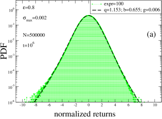
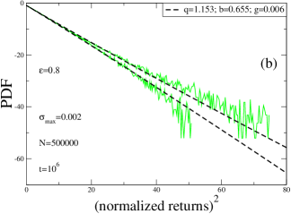
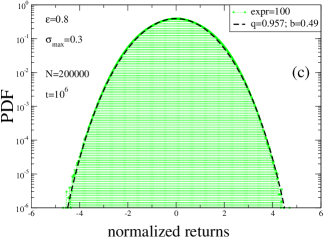
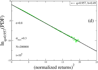
Figure 4: Asymptotic PDFs of the normalized returns with large $N$ and large number of time steps for $\sigma_{max}=0.002$ (a) and $\sigma_{max}=0.3$ (c). For both cases $\tau=32$. The $q$-logarithms versus the square of normalized returns have already been given for both cases in (b) and (d) respectively.

II $q$-Gaussian approximants

Let us now attempt a wider look at the same problem, by extending the preliminary results given in Alex2013 . A simple $q$-Gaussian approximant describes fairly well the numerical data unless we focus on a parameter value where an asymmetry emerges in the PDF. The index $q$ is generically expected to depend on $(\epsilon,\sigma_{max},\tau)$.

First of all, we need to define the procedure that we are employing in order to predict the best value of $q$ parameter of the related $q$-Gaussian at each tuple. The $q$-Gaussians can be obtained by optimising the entropy $S_{q}=\left(1-\sum_{i=1}^{W}p_{i}^{q}\right)/(q-1)$ tsallis1 and can be given for $-\infty<q<3$ as

$$p=A_{q}\sqrt{B_{q}}\,e_{q}^{-B_{q}x^{2}}$$ (7)

where $e_{q}^{y}$, known as $q$-exponential, is defined by

$$e_{q}^{y}=\left\{\begin{array}[]{ll}\left[1+(1-q)y\right]^{1/(1-q)}\,\,\,,&\,\,\,\mbox{$1+(1-q)y\geq 0$}\\ \,\,\,\,\,\,\,\,\,\,\,\,\,\,\,\,\,\,0\,\,\,\,\,\,\,\,\,\,\,\,\,\,\,\,\,\,\,\,\,\,\,\,\,\,\,\,\,\,\,\,\,,&\,\,\,\,\,\,\,\,\,\,\,\,\,\,\,\,\,\,\mbox{else}\,.\end{array}\right.$$ (8)

By inverting this function we obtain the $q$-logarithm function defined above.

The $q$-dependent coefficient $A_{q}$ in Eq. (7) is given by

$$A_{q}=\left\{\begin{array}[]{ll}\frac{\Gamma\left(\frac{5-3q}{2-2q}\right)}{\Gamma\left(\frac{2-q}{1-q}\right)}\sqrt{\frac{1-q}{\pi}}\,\,\,,&\,\,\,\mbox{$q<1$}\\ \frac{1}{\sqrt{\pi}}\,\,\,,&\,\,\,\mbox{$q=1$}\\ \frac{\Gamma\left(\frac{1}{q-1}\right)}{\Gamma\left(\frac{3-q}{2q-2}\right)}\sqrt{\frac{q-1}{\pi}}\,\,\,,&\,\,\,\mbox{$1<q<3$}\,.\end{array}\right.$$ (9)

The quantity $B_{q}$ characterizes the PDF width $w$ of the distribution as follows:

$$B_{q}=\frac{1}{(3-q)w}\,\,,$$ (10)

where $w$ is, for $q<5/3$, related to the standard deviation $s$ through

$$(5-3q)s^{2}=(3-q)w^{2}\,\,.$$ (11)

In our simulations, there are only two free parameters, namely $q$ and $B_{q}$, to be adjusted under the assumption that the number of decades that we are observing still shows a symmetric PDF. For a given set $(\epsilon,\sigma_{max},\tau)$, we adjust the best value of $q$ by looking at the curves $\ln_{q}$(PDF) versus (normalized returns)². The procedure consists in determining the value of $q$ which provides the best approach to a straight line. More precisely, we fit the curves resulting from various values of $q$ with a quadratic function

$$y=\alpha+\beta x+\gamma x^{2}\,\,,$$ (12)

and choose the value of $q$ which provides the minimal value for the parameter $\gamma$. Then, for this $q$ value, we calculate $A_{q}$ and $B_{q}$ parameters from the time series. Finally, using all these obtained parameter values, we plot the best $q$-Gaussian for the chosen set $(\epsilon,\sigma_{max},\tau)$. Two typical examples are given in Fig. 5. For these examples, the minimal value of $\gamma$, denoted by $\gamma_{min}$, have been obtained for $q=0.964$ and $q=1.022$, respectively. Then these values of $q$ have been used to determine the values of the $A_{q}$ and $B_{q}$ parameters. Finally, the PDFs of the normalized returns are approached as shown in Fig. 5b and 5d. It is evident from the figure that the best $q$-Gaussian approximants corroborate the behaviour of the system for more than 6 decades in each case. The obtained results are summarized in Table I and plotted in Fig. 6 for typical values of $(\epsilon,\sigma_{max})$. Unless the $\sigma_{max}$ values are very small, the tendency is always towards a $q$-Gaussian with $q<1$. For very small $\sigma_{max}$, $q>1$ are also observed but for such cases the asymmetry becomes important.

In our simulations, we prefer to set $\tau=128$ since it is evident from Fig. 7 that if $\tau$ is not very small the PDF remains the same as $\tau$ is increased.

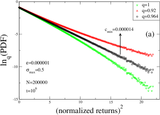
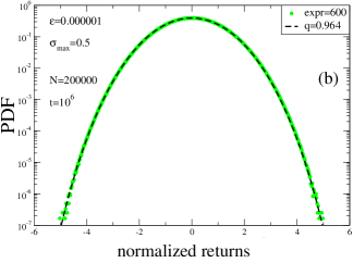
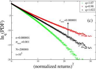
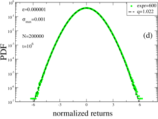
Figure 5: Two typical examples of choosing the most appropriate $q$ value using the quadratic function for a case $q<1$ (a) and for a case $q>1$ (c). The appropriate $q$ value is taken as the one that gives the smallest $\gamma$ value (denoted as $\gamma_{min}$). The probability density of the same examples using the $q$ value obtained from the explained procedure for the case $q<1$ (b) and for the case $q>1$ (d).

$\epsilon=0.000001$
$\sigma_{max}$	$A_{q}\sqrt{B_{q}}$	$B_{q}$	$q$
0.001	0.4023	0.5171	1.022
0.05	0.3957	0.4840	0.978
0.1	0.3989	0.4897	0.986
0.2	0.3944	0.4771	0.968
0.3	0.3944	0.4771	0.968
0.4	0.3953	0.4819	0.975
0.5	0.3938	0.4744	0.964
0.6	0.3937	0.4737	0.963
0.7	0.3930	0.4704	0.958

$\epsilon=0.8$
$\sigma_{max}$	$A_{q}\sqrt{B_{q}}$	$B_{q}$	$q$
0.0015	0.4214	0.6154	1.125
0.02	0.4077	0.5441	1.054
0.15	0.3912	0.4613	0.944
0.2	0.3888	0.4494	0.925
0.3	0.3926	0.4684	0.955
0.4	0.3912	0.4613	0.944
0.45	0.3885	0.4482	0.923
0.5	0.3873	0.4423	0.913
0.55	0.3950	0.4805	0.973

Table 1: For $\tau=128$ and two typical values of $\epsilon$, the values of the parameters $A_{q}\sqrt{B_{q}}$, $B_{q}$ and $q$ as $\sigma_{max}$ varies are indicated.

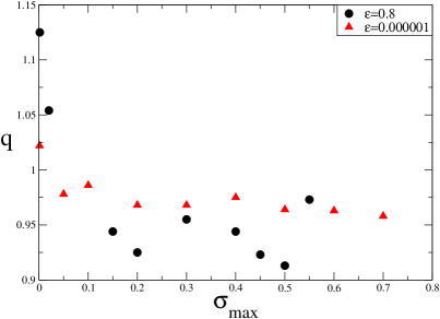
Figure 6: The behaviour of the index $q$ as a function of $\sigma_{max}$ for two typical values of $\epsilon$.

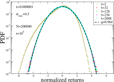
Figure 7: The effect of $\tau$ on the behavior of the PDF.

We have also checked the effect of $\epsilon$ for a fixed value of $\sigma_{max}$. A clear tendency of increasing $q$ values as $\epsilon$ is decreasing has been observed with a saturation value around $q\simeq 0.965$ as given in Table II and plotted in Fig. 8.

$\sigma_{max}=0.5$
$\epsilon$	$A_{q}\sqrt{B_{q}}$	$B_{q}$	$q$
0.000001	0.3938	0.4744	0.964
0.00001	0.3937	0.4737	0.963
0.0001	0.3941	0.4757	0.966
0.001	0.3939	0.4751	0.965
0.01	0.3939	0.4751	0.965
0.1	0.3914	0.4625	0.946
0.2	0.3895	0.4531	0.931
0.5	0.3878	0.4446	0.917
0.8	0.3873	0.4423	0.913

Table 2: For $\tau=128$ and a typical value of $\sigma_{max}$, the values of the parameters $A_{q}\sqrt{B_{q}}$, $B_{q}$ and $q$ as $\epsilon$ varies are indicated.

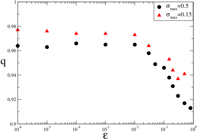
Figure 8: The behaviour of the index $q$ as a function of $\epsilon$ for a typical value of $\sigma_{max}$.

Finally, we have simulated the case $\mu=2$ without noise. As expected, in this case, a clear Gaussian with 6 decades can be seen in Fig. 9 since all individual logistic maps are at their mostly chaotic points. Whenever a nonzero noise term is included, the system is not able to achieve the Gaussian due to the persistence of the noise on each map.

Figure 9: The behaviour of the PDF for a typical case of $\mu=2$.

III Conclusions

We have numerically studied, along many decades, the time-averaged returns in the model recently introduced in Alex2013 by varying the number $N$ of logistic maps in the chain, the first-neigbour-coupling constant $\epsilon$, the width $\sigma_{max}$ of the common noise, and the characteristic return time $\tau$.

Our results can be summarised as follows. When the control parameter $\mu$ of the logistic maps is taken to be close to the edge of chaos ($\mu_{c}$), where the Lyapunov exponent vanishes, slightly asymmetric distributions are observed for some parameter values. Unless the number of decades is quite large, this asymmetry can be neglected and the distributions satisfactorily admit $q$-Gaussian approximants even for these parameter values. We have illustrated the effect on the index $q$ of the various parameters of the model.

When we choose for the parameter $\mu$ of the logistic maps not its value at the edge of chaos but any other value such that the Lyapunov exponent is positive, we obtain numerical PDFs that, as expected, are well fitted by simple Gaussians along six PDF decades when the system has no noise. In the presense of noise, however, the system is unable to achieve the Gaussian PDF due to the persistent perturbation of the noise.

The overall scenario is that, when we consider time-averaged relevant quantities such as the returns, Boltzmann-Gibbs statistics (with its Gaussians, consistent with the classical Central Limit Theorem) emerges when strong chaos (positive Lyapunov exponent) is present, and nonextensive statistical mechanics (with its $q$-Gaussians, consistent with the $q$-generalized Central Limit Theorem qCLT ) emerges, or nearly emerges, when weak chaos (zero Lyapunov exponent) is present. These facts reinforce the results recently obtained with time-averaged quantities for the (conservative) standard map TirnakliBorges2014 . Biological and other systems appear to be well mimicked by the Pluchino et al model Alex2013 . The present results might be useful for examining such systems.

References

- (1) S.H. Strogatz, Sync: The Emerging Science of Spontaneous Order (Hyperion, New York, 2004).
- (2) A. Pikovski, M. Rosenblum and J. Kurths, Synchronization: A Universal Concept in Nonlinear Sciences (Cambridge University Press, Cambridge, 2001).
- (3) K. Kaneko, Simulating Physics with Coupled Map Lattices (World Scientific, Singapore, 1990).
- (4) T. Shibata, T. Chawanya and K. Kaneko, Phys. Rev. Lett. 82, 4424 (1999).
- (5) J.N. Teramae and Y. Kuramoto, Phys. Rev. E 63, 036210 (2001).
- (6) A. Pluchino, A. Rapisarda and C. Tsallis, Phys. Rev. E 87, 022910 (2013).
- (7) M. De Menech and A.L. Stella, Physica A 309, 289 (2002).
- (8) M.I. Bogachev and A. Bunde, Phys. Rev. E 78, 036114 (2008).
- (9) J. Ludescher, C. Tsallis and A. Bunde, Europhys. Lett. 95, 68002 (2011).
- (10) M.I. Bogachev, A.R. Kayumov and A. Bunde, PLoS ONE 9 (12), e112534 (2014).
- (11) F. Caruso, A. Pluchino, V. Latora, S. Vinciguerra, and A. Rapisarda, Phys. Rev. E 75, 055101(R) (2007).
- (12) B. Bakar and U. Tirnakli, Phys. Rev. E 79, 040103(R) (2009).
- (13) B. Bakar and U. Tirnakli, Physica A 389, 3382 (2010).
- (14) A. Celikoglu, U. Tirnakli and S.M.D. Queiros, Phys. Rev. E 82, 021124 (2010).
- (15) C. Tsallis, Introduction to Nonextensive Statistical Mechanics: Approaching a Complex World (Springer, New York, 2009).
- (16) S. Umarov, C. Tsallis and S. Steinberg, Milan J. Math. 76, 307 (2008); S. Umarov, C. Tsallis, M. Gell-Mann and S. Steinberg, J. Math. Phys. 51, 033502 (2010).
- (17) U. Tirnakli and E.P. Borges, "The standard map: From Boltzmann-Gibbs statistics to Tsallis statistics", arXiv: 1501.02459, (2015).