FTPI-MINN-15-14, UMN-TH-3428-15

’t Hooft-Polyakov Monopoles with Non-Abelian Moduli

M. Shifman^a, G.Tallarita^b,c, and A. Yung^a,d

^aWilliam I. Fine Theoretical Physics Institute, University of Minnesota, Minneapolis, MN 55455, USA
^bCentro de Estudios Científicos (CECs), Casilla 1469, Valdivia, Chile

^cDepartmento de Física, Universidad de Santiago de Chile, Casilla 307, Santiago, Chile

^dNational Recearch Center “Kurchatov Institute”, Petersburg Nuclear Physics Institute, Gatchina, St. Petersburg 188300, Russia

Abstract

We extend the Georgi-Glashow model of the t’Hooft-Polyakov monopoles to include additional collective coordinates “orientational isospin moduli.” The low-energy theory of these solitonic solutions can be interpreted as dyons with isospin.

1 Introduction

Magnetic monopole is one of the most venerable constructions in theoretical physics. It dates back to Dirac [2]. Implementation of this construction in field theory is due to ’t Hooft [3] and Polyakov [4] (for reviews and references see e.g. [5, 6, 7]). Remarkable effects were shown to be associated with the ’t Hooft-Polyakov monopoles, e.g. the Callan-Rubakov effect of the baryon decay catalysis [8, 9, 10]. In the monopole field $SU(2)_{\rm gauge}$ doublet fermions acquire integer spin (e.g. [6]). This phenomenon is called “spin from isospin.”

In this paper we will consider an extension of the Georgi-Glashow model [11], in which a global $O(3)$ (“isospin”) symmetry is present in the Lagrangian. A simple model possessing this property and suitable for our purposes was suggested in [12] (see also [13]). Conceptually it was inspired by Witten’s cosmic strings [14]. Our task is to demonstrate that in this model the ’t Hooft-Polyakov monopole acquires additional collective coordinates, isospin moduli. The overall set of collective coordinates includes three coordinates of the monopole center, a $U(1)$ phase coordinate which, upon quantization, corresponds to the electric charge and produces dyons out of the monopoles, and two extra collective coordinates associated with the $O(3)$ isospin. Quantization of the isospin collective coordinates is straightforward, paralleling that of the spherical quantum top.

2 The model

Our starting point is the well-known Georgi-Glashow model [11]. The gauge group is $SU(2)$ and the matter sector is described by a triplet real field $\phi^{a}$ (belonging to the adjoint representation). The Lagrangian of this model is

$$\mathcal{L}_{\rm GG}=-\frac{1}{4g^{2}}G^{a}_{\mu\nu}G^{\mu\nu,a}+\frac{1}{2}(D_{\mu}\phi^{a})(D^{\mu}\phi^{a})-\lambda\left(\phi^{a}\phi^{a}-v^{2}\right)^{2},$$ (1)

where

$$D_{\mu}\phi^{a}=\partial_{\mu}\phi^{a}+\varepsilon^{abc}A^{b}_{\mu}\phi^{c},$$ (2)

is the covariant derivative in the adjoint representation, and

$$G^{a}_{\mu\nu}=\partial_{\mu}A^{a}_{\nu}-\partial_{\nu}A^{a}_{\mu}+\varepsilon^{abc}A^{b}_{\mu}A^{c}_{\nu}$$ (3)

is the non-Abelian field strength. We use the following matrix notation for the fields

$$\phi=\phi^{a}\frac{\tau_{a}}{2},$$ (4)

where $\tau_{a}$ denote the standard Pauli matrices. In the Lagrangian, $v$ is a parameter with dimensions of mass, and $\lambda$ is a dimensionless coupling constant. As is well known, this model supports the t’Hooft-Polyakov magnetic monopoles [3, 4] that are topologically stable as a consequence of the symmetry breaking pattern

$$SU(2)_{\rm gauge}\rightarrow U(1)_{\rm gauge}\,.$$ (5)

The breaking (5) is enforced by the non-vanishing vacuum expectation value of the $\phi$ field, which can always be chosen aligned in the $3$-direction in $SU(2)_{\rm gauge}$,

$$\phi^{a}_{vac}=v\delta^{3a}\,.$$ (6)

Two components of the gauge field, called $W^{\pm}$, acquire masses

$$m_{W}=gv\,,$$ (7)

whilst the component aligned along the vacuum direction remains massless and plays the role of the $U(1)$ photon. The mapping between the group space and the coordinate space at infinity can be classified by the second homotopy class,

$$\pi_{2}\left(SU(2)/U(1)\right)=\mathbb{Z},$$ (8)

which guarantees the topological stability of the monopoles.

Historically, the introduction of non-Abelian moduli on topological defects occurred in a rather advanced settings, mostly involving supersymmetric gauge theories (see [15, 16, 17]). In [12] a much simpler setup was suggested resulting in the occurrence of non-Abelian moduli. We will use this setup to study non-Abelian moduli on the world-line of the t’Hooft-Polyakov monopoles. To this end we will end a term $\mathcal{L}_{\chi}$ to the Lagrangian (1),

$$\mathcal{L}=\mathcal{L}_{\rm GG}+\mathcal{L}_{\chi}$$ (9)

where

$$\mathcal{L}_{\chi}=\partial_{\mu}\chi^{i}\partial^{\mu}\chi^{i}-\gamma\left[(-\mu^{2}+\phi^{a}\phi^{a})\chi^{i}\chi^{i}+\beta(\chi^{i}\chi^{i})^{2}\right].$$ (10)

Here $\chi^{i}$ is an $O(3)$ triplet uncharged under the gauge group. The potential term coupling $\chi^{i}$ to $\phi^{a}$ ensures that, if $\mu<v$, the $\chi^{i}$ field will develop in the monopole core and vanish in the vacuum. The mass of the $\chi$ field is

$$m_{\chi}^{2}=\gamma(v^{2}-\mu^{2}).$$ (11)

The global $O(3)$ symmetry of (10) is obvious.

Now, assuming the standard monopole ansatz for the fields $\phi$ and $A$

$$\phi^{a}=vn^{a}H(r),\quad A_{i}^{a}=\epsilon^{aij}\frac{1}{r}n^{j}F(r),$$ (12)

with $n^{a}=x^{a}/r$, and adding a self-evident ansatz for $\chi^{i}$,

$$\chi^{i}=\sqrt{\frac{\mu^{2}}{2\beta}}\;\chi(r)\;\left(\begin{array}[]{l}0\\ 0\\ 1\end{array}\right),$$ (13)

we can reduce the energy functional to

$$E = \frac{4\pi v}{g}\int_{0}^{\infty}d\rho\rho^{2}\bigg{[}\frac{(F^{\prime})^{2}}{\rho^{2}}+\frac{(2F-F^{2})^{2}}{2\rho^{4}}+\frac{H^{2}(1-F)^{2}}{\rho^{2}}+\frac{(H^{\prime})^{2}}{2}$$ (14)

$$+\frac{\lambda}{g^{2}}\left(H^{2}-1\right)^{2}+\frac{\tilde{\mu}^{2}}{2\beta}\left((\chi^{\prime})^{2}+\frac{\gamma}{g^{2}}\left[(-\tilde{\mu}^{2}+H^{2})\chi^{2}+\frac{\tilde{\mu}^{2}}{2}\chi^{4}\right]\right)\bigg{]},$$

in dimensionless units

$$\rho=gv|\vec{x}|\,.$$ (15)

Here $\tilde{\mu}$ is dimensionless,

$$\tilde{\mu}=\mu/v.$$ (16)

The energy minimization equations are

$$\left(\rho^{2}H^{\prime}\right)^{\prime} = H\left[2(F-1)^{2}+\frac{4\lambda\rho^{2}}{g^{2}}\left(H^{2}-1\right)+\frac{\gamma\tilde{\mu}^{2}\rho^{2}}{g^{2}\beta}\chi^{2}\right],$$ (17)

$$\rho^{2}F^{\prime\prime} = (-1+F)\left((-2+F)F+\rho^{2}H^{2}\right),$$ (18)

$$\left(\rho^{2}\chi^{\prime}\right)^{\prime} = \frac{\gamma\rho^{2}}{g^{2}}\chi\left(H^{2}+\tilde{\mu}^{2}\left(-1+\chi^{2}\right)\right).$$ (19)

2.1 Vacuum structure

In the vacuum, all derivatives of the profile functions must vanish. Clearly equation (18) imposes the condition that $F=1$ in the vacuum. This leads to four branches of extrema of the energy, the first is

$$H^{I}_{vac}=\chi^{I}_{vac}=0,$$ (20)

this is a maximum of the energy functional with $E^{I}_{max}/4\pi v=\lambda/g^{3}$. Then, in the vacuum II,

$$H^{II}_{vac}=1,\quad\chi^{II}_{vac}=0,$$ (21)

for which the vacuum energy density vanishes $E^{II}_{vac}=0$. The third branch is

$$H^{III}_{vac}=0,\quad\chi^{III}_{vac}=1,$$ (22)

for which

$$\frac{E^{III}_{vac}}{4\pi v}=\frac{1}{g^{3}}\left(\lambda-\frac{\tilde{\mu}^{4}\gamma}{4\beta}\right).$$ (23)

Finally, the fourth branch is

$$(H^{IV}_{vac})^{2}=\frac{4\beta\lambda-\gamma\tilde{\mu}^{2}}{4\beta\lambda-\gamma},\quad(\chi^{IV}_{vac})^{2}=\frac{4\beta\lambda(1-\tilde{\mu}^{2})}{\tilde{\mu}^{2}(\gamma-4\beta\lambda)}$$ (24)

for which

$$\frac{E^{IV}_{vac}}{4\pi v}=\frac{\gamma\lambda}{g^{3}}\frac{(\tilde{\mu}^{2}-1)^{2}}{\gamma-4\beta\lambda}.$$ (25)

Hence, when $\gamma<4\beta\lambda$ this branch corresponds to the actual vacuum. The branches $II$ and $IV$ meet at $\tilde{\mu}=1$, or when $\mu=v$. When $\gamma>4\beta\lambda$ and $\lambda>\frac{\tilde{\mu}^{4}\gamma}{4\beta}$ the vacuum $II$ is the actual vacuum.

Below we look for solutions in vacuum $II$.

3 Numerical results

Here we present the solutions of (17)-(19) obtained by a second order central finite difference numerical procedure with the accuracy ${O}(10^{-4})$. To launch our numerical procedure we cut-off the radial direction at a large value of $\rho$, which we will call $R$. We set $R=100$. As an example we choose the following values of the parameters:

$$\gamma=4,\quad\lambda=0.34,\quad\tilde{\mu}=0.999,\quad\beta=2.94,\quad g=0.6\,.$$ (26)

Our boundary conditions are

$$H(0)=F(0)=0,\quad\chi^{\prime}(0)=0,$$ (27)

$$H(R)=F(R)=1,\quad\chi(R)=0.$$ (28)

The sought for solution is shown in Figure 1. The energy (monopole mass) $M_{M}$ of this solution is

$$\frac{M_{M}}{4\pi v}=2.14\,,\qquad\mbox{Monopole with the isospin}.$$ (29)

The mass $M_{M}$ of the standard t’Hooft-Polyakov monopole at $\lambda=0.34$ and $g=0.6$ is

$$\frac{M_{M}}{4\pi v}=2.33\,.$$ (30)

Thus, the energy of the monopole with the nonvanishing $\chi^{i}$ in the core is lower.

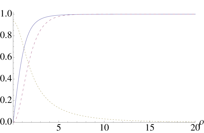
Figure 1: Non-Abelian monopole profiles for $\gamma=4$, $\lambda=0.34$, $\tilde{\mu}=0.999$, $\beta=2.94$ and $g=0.6$. The solid curve represents $H$, medium dashed $F$ and thin dashed $\chi$.

4 Stability

In this section we can check that the solution found above with a nonvanishing $\chi$ in the core is stable. The energy functional for the $\chi$ field is

$$E_{\chi}=\frac{4\pi v}{g}\int_{0}^{\infty}d\rho\rho^{2}\left[(\chi^{\prime})^{2}+\frac{\gamma}{g^{2}}\left((-\tilde{\mu}^{2}+H^{2})\chi^{2}+\frac{\tilde{\mu}^{2}}{2}\chi^{4}\right)\right].$$ (31)

Introducing

$$\psi(\rho)=\rho\chi$$ (32)

we can derive a one-dimensional Schrödinger-like equation for the $\psi$ eigenfunctions,

$$-\psi^{\prime\prime}+\frac{\gamma}{g^{2}\rho^{2}}\left((-\tilde{\mu}^{2}+H_{1}^{2})+3\tilde{\mu}^{2}\chi_{1}^{2}\right)\psi=\epsilon\psi$$ (33)

where $H_{1}$ and $\chi_{1}$ are the field profiles shown in Figure 1. Using the same parameters as in (26) we find the lowest-lying mode at $\epsilon\approx 0.00105$. The positivity of $\epsilon$ demonstrates the stability of the numerical solution with a non-vanishing $\chi$ field in the core.

Since the solution with a non-zero $\chi$ in the core has lower energy than the vanishing-$\chi$ solution we must also investigate (meta)stability of the vanishing-$\chi$ solution. Then, following the argument above, we must solve

$$-\psi^{\prime\prime}+\frac{\gamma}{g^{2}\rho^{2}}(-\tilde{\mu}^{2}+H_{1}^{2})\psi=\epsilon\psi\,.$$ (34)

We find that the lowest lying mode is at $\epsilon\approx 0.00103$ thus confirming the classical stability of the $\chi=0$ solution.

Thus, we observe two classical solutions: one – the standard ’t Hooft-Polyakov monopole is a local minimum of the energy functional, while the solution with the nonvanishing $\chi$ in the core represents the global minimum.

5 Quantization of the collective coordinates

Quantization of the standard t’Hooft-Polyakov monopole involves four moduli: three translations of the monopole center plus a rotation around the vacuum direction in the $SU(2)_{\rm gauge}$ space. In the adiabatic approximation one finds the Lagrangian

$$\mathcal{L}_{QM}=-M_{M}+\frac{M_{M}}{2}(\dot{\vec{x_{0}}})^{2}+\frac{1}{2}\frac{M_{M}}{m^{2}_{W}}\dot{\alpha}^{2}$$ (35)

where $M_{M}$ is the mass of the monopole, the vector $\vec{x_{0}}$ represents the monopole center, whilst $\alpha$ is the collective coordinate related to the remaining $U(1)_{\rm gauge}$ invariance. The full quantum mechanical Hamiltonian for these moduli is

$$\widehat{H}_{0}=M_{M}+\frac{\vec{p}\;^{2}}{2M_{M}}+\frac{1}{2}\frac{m_{W}^{2}}{M_{M}}\pi^{2}_{\alpha},$$ (36)

where

$$\pi_{\alpha}=\frac{M_{M}}{m^{2}_{W}}\dot{\alpha},$$ (37)

is the canonical momentum conjugated to the angular variable $\alpha$.

To obtain the orientational moduli we parametrize the $\chi$ field as follows

$$\chi^{i}=\sqrt{\frac{\mu^{2}}{2\beta}}\chi(\rho)S^{i}(t)$$ (38)

where $S^{i}$ is a unit vector which depends on time. Substituting (38) in (14) we obtain the low-energy action for the orientational moduli,

$$\mathcal{S}_{0}=\frac{I_{1}}{2}\int dt\;\dot{S}^{i}\dot{S}^{i},\quad S^{i}S^{i}=1,$$ (39)

where

$$\frac{I_{1}v}{4\pi}=\frac{\tilde{\mu}^{2}}{g^{3}\beta}\int_{0}^{\infty}d\rho\,\rho^{2}\chi^{2}=7.81,$$ (40)

and the overdot denotes a derivative with respect to time. The above action can be easily quantized as follows.

The action (39) describes the motion of a rigid rotating body, symmetric quantum top, at a fixed spherical radius $r_{0}$ (in this case $r_{0}=1$). Its quantization can be carried out in a standard way (see. e.g. [18]), if we parametrize $S^{i}$ in terms of polar and azimuthal angles,

$$S^{1}=\cos\theta\,,\quad S^{2}=\sin\theta\,\cos\varphi\,,\quad S^{3}=\sin\theta\,\sin\varphi\,.$$ (41)

Upon quantization we get the following symmetric top Hamiltonian:

$$\widehat{H}=-\frac{1}{2I_{1}}\left[\frac{1}{\sin{\theta}}\frac{\partial}{\partial\theta}\left(\sin{\theta}\frac{\partial}{\partial\theta}\right)+\frac{1}{\sin^{2}\theta}\frac{\partial^{2}}{\partial\varphi^{2}}\right].$$ (42)

Its eigenvalues are labelled by a non-negative integer $s$ and reduce to

$$E_{s}=\frac{1}{2I_{1}}s\left(s+1\right)\,.$$ (43)

They have degeneracy $2s+1$. The eigenfunctions are the standard spherical harmonics $Y_{s}\left(\theta,\varphi\right)$.

Including the conventional ’t Hooft-Polyakov moduli from Eq. (36) we arrive at the monopole mass formula

$$M=M_{M}+\frac{m_{W}^{2}\,k^{2}}{2M_{M}}\ +\frac{1}{2I_{1}}\,s(s+1),$$ (44)

where $k$ and $s$ are integers. The $k^{2}$ term here corresponds to dyonic excitations associated with non-zero electric charge, while the last term is associated with non-zero global isospin. The $I_{1}$ parameter plays the role of the moment of inertia in the isospace. With our illustrative choice of parameters $I_{1}^{-1}\sim(1/60)m_{W}$ while $m_{W}/M_{M}\sim 1/40.$

6 Conclusions

In this model we completed the program of constructing the simplest topological defects with non-Abelian moduli. We extended the Georgi-Glashow model of the t’Hooft-Polyakov monopoles to include extra global symmetry $O(3)$ (we referred to it as isospin) and extra collective coordinates “orientational isospin moduli.” The adiabatic quantization of these solitonic solutions was carried out. The result can be interpreted as a dyon with isospin.

References

- [1]
- [2] P. Dirac, Quantised Singularities in the Electromagnetic Field, Proc. Roy. Soc. (London) A 133, 60 (1931).
- [3] G. ’t Hooft, Magnetic Monopoles in Unified Gauge Theories, Nucl. Phys. B 79, 276 (1974).
- [4] A. M. Polyakov, Particle Spectrum in the Quantum Field Theory, JETP Lett. 20, 194 (1974).
- [5] Eric Weinberg, Classical Solutions in Quantum Field Theory, (Cambridge University Press, 2012).
- [6] V. A. Rubakov, Classical theory of gauge fields, (Princeton University Press, 2002).
- [7] M. Shifman, Advanced Topics in Quantum Field Theory, (Cambridge University Press, 2012).
- [8] V. A. Rubakov, Adler-Bell-Jackiw Anomaly and Fermion Number Breaking in the Presence of a Magnetic Monopole, Nucl. Phys. B 203, 311 (1982).
- [9] C. G. Callan, Jr., Monopole Catalysis of Baryon Decay, Nucl. Phys. B 212, 391 (1983).
- [10] C. G. Callan, Jr. and E. Witten, Monopole Catalysis of Skyrmion Decay, Nucl. Phys. B 239, 161 (1984).
- [11] H. Georgi and S. L. Glashow, Unified weak and electromagnetic interactions without neutral currents, Phys. Rev. Lett. 28, 1494 (1972).
- [12] M. Shifman, Simple Models with Non-Abelian Moduli on Topological Defects, Phys. Rev. D 87, no. 2, 025025 (2013) [arXiv:1212.4823 [hep-th]].
- [13] M. Shifman and A. Yung, Abrikosov-Nielsen-Olesen String with Non-Abelian Moduli and Spin-Orbit Interactions, Phys. Rev. Lett. 110, no. 20, 201602 (2013) [arXiv:1303.7010 [hep-th]].
- [14] E. Witten, Superconducting Strings, Nucl. Phys. B 249, 557 (1985).
- [15] A. Hanany and D. Tong, Vortices, instantons and branes, JHEP 0307, 037 (2003) [hep-th/0306150]; R. Auzzi, S. Bolognesi, J. Evslin, K. Konishi and A. Yung, Non-Abelian superconductors: Vortices and confinement in SQCD, Nucl. Phys. B 673, 187 (2003) [hep-th/0307287]; M. Shifman, A. Yung, NonAbelian string junctions as confined monopoles, Phys. Rev. D70, 045004 (2004). [hep-th/0403149]; A. Hanany and D. Tong, Vortex strings and four-dimensional gauge dynamics, JHEP 0404, 066 (2004) [hep-th/0403158].
- [16] M. Shifman and A. Yung, Supersymmetric Solitons, (Cambridge University Press, 2009).
- [17] A. Gorsky, M. Shifman and A. Yung, Non-Abelian Meissner effect in Yang-Mills theories at weak coupling, Phys. Rev. D 71, 045010 (2005) [hep-th/0412082]; A. Gorsky and V. Mikhailov, Nonabelian strings in a dense matter, Phys. Rev. D 76, 105008 (2007) [arXiv:0707.2304 [hep-th]]; Non-Abelian Strings in Hot or Dense QCD, Prog. Theor. Phys. Suppl. 174, 254 (2008) [arXiv:0805.4539 [hep-ph]]; M. Eto, M. Nitta and N. Yamamoto, Instabilities of Non-Abelian Vortices in Dense QCD, Phys. Rev. Lett. 104, 161601 (2010) [arXiv:0912.1352 [hep-ph]]; A. Gorsky, M. Shifman and A. Yung, Confined Magnetic Monopoles in Dense QCD, Phys. Rev. D 83, 085027 (2011) [arXiv:1101.1120 [hep-ph]].
- [18] A. Losev, M. A. Shifman and A. I. Vainshtein, Single state supermultiplet in (1+1)-dimensions, New J. Phys. 4, 21 (2002) [hep-th/0011027].
- [19]