Statistical properties of Charney-Hasegawa-Mima zonal flows

Abstract

A theoretical interpretation of numerically generated probability density functions (PDFs) of intermittent plasma transport events in unforced zonal flows is provided within the Charney-Hasegawa-Mima (CHM) model. The governing equation is solved numerically with various prescribed density gradients that are designed to produce different configurations of parallel and anti-parallel streams. Long-lasting vortices form whose flow is governed by the zonal streams. It is found that the numerically generated PDFs can be matched with analytical predictions of PDFs based on the instanton method by removing the autocorrelations from the time series. In many instances the statistics generated by the CHM dynamics relaxes to Gaussian distributions for both the electrostatic and vorticity perturbations, whereas in areas with strong nonlinear interactions it is found that the PDFs are exponentially distributed.

I Introduction

In recent experiments and numerical simulations it has been found that significant transport might be mediated by coherent structures such as streamers, blobs and vortices through the formation of rare avalanche-like events of large amplitude zweben2007 ; politzer2000 ; beyer2000 ; drake1988 ; antar2001 ; carreras1996 ; nagashima2011 ; dif2010 . These events cause the probability distribution function (PDF) to deviate from a Gaussian profile on which the traditional mean field theory such as transport coefficients is based. Specifically, the PDF tails manifest the intermittent character of transport due to rare events of large amplitude that are often found to substantially differ from Gaussian distribution, although PDF centres tend to be Gaussian. Therefore, a comprehensive predictive theory is called for in order to understand and subsequently improve intermittent transport features e.g. confinement degradation in tokamaks.

Drift wave turbulence is known to generate zonal flows, which in turn inhibits the growth of turbulence and transport DiamondEA2005 ; DiamondEA2011 . As such, zonal flows play an important role in fusion plasmas ConnorEA2004 ; ItohEA2006 ; ConnorMartin2007 .

In geophysical fluid dynamics, zonal flows are believed to cause a similar reduction in transport in atmospheres SmedmanEA2004 ; PrabhaEA2008 under certain limiting conditions DuarteEA2012 . This comes as no surprise, given the analogy between drift waves in the dissipationless limit and Rossby waves in nearly incompressible, shallow rotating fluids; both systems are described by the Charney-Hasegawa-Mima (CHM) equation hi1996 .

Numerical studies where sheared flow is externally prescribed CarrerasEA1992 ; GarbetEA2002 ; TynanEA2006 lead to energetics that are qualitatively different from those obtained in the drift-wave/zonal-flow feedback mechanism ConnaughtonEA2011 . In the CHM model charney1948 ; hm1977 ; hm1978 sheared flow may be imposed by prescribing the background density gradient botha1999 . The known solutions of the CHM equation, namely bipolar and monopolar vortices Nycander1988 , form in the plasma. Here the term vortex is used to describe a localized extremum in the electrostatic potential that is evolved through the CHM equation. In this paper fluid simulations using the CHM equation are designed so that zonal flows

are prescribed externally,

moving in the poloidal direction and with various configurations in the radial direction. At initialisation bipolar vortices form, but only monopolar vortices survive due to the interaction between vortices as well as the destructive effects of the sheared flow hi1996 .

The fluid simulations produce quasi-stationary time series (poloidally averaged and sampled at different radial points) of the electrostatic potential and corresponding vorticity that describe the CHM flows horton1999 ; charney1948 ; hm1977 ; hm1978 ; hmk1979 ; botha1999 . We apply a standard Box-Jenkins modeling for each time series. This mathematical procedure effectively removes deterministic autocorrelations from the time series, allowing for the statistical interpretation of the stochastic residual part. In this particular case it turns out that an ARIMA(3,1,0) model (autoregressive integrated moving average) box1994 accurately describes the stochastic process.

The stochastic residual of the time series of potential and vorticity exhibit Gaussian statistics or distributions with elevated exponential tails. We utilize analytical results from nonperturbative stochastic theory, the so-called instanton method justin1989 ; gurarie1996 ; falcovich1996 ; kim2002 ; anderson1 ; kim2008 ; anderson2 for computing PDFs in turbulence as a comparison to the numerical data. The analytically derived PDFs are rather insensitive to the details of the linear physics of the system kim2008 and thus display salient features of the nonlinear interactions. The numerically generated time traces are analysed using the ARIMA model and fitted with the analytical models accordingly. We find in the regions with strong nonlinear characteristics an emergent universal scaling of the PDF tails of exponential form $\sim\exp\big{(}-const\ |\phi|\big{)}$ as suggested by recent theoretical work in Ref. falcovich2011, ; kim2008, ; anderson4, relevant for the direct cascade dynamics. However, in many cases for the CHM zonal flows we find Gaussian PDFs in similarity to what was seen from the theoretical model in Ref. anderson3, , whereas for some mid radial points the system exhibit sub-exponential PDFs $\sim\exp\big{(}-const\ |\phi|^{\alpha}\big{)}$ with $\alpha<1$, where the dynamics is strongly influenced by the zonal flow resulting in strong intermittency.

The paper is organized as follows: Section II introduces the CHM model and Section III the statistical method used in the analysis. The numerical results are presented in Section IV after which they are discussed and the paper is concluded by a summary of the main results.

II Charney-Hasegawa-Mima model

The CHM equation is solved in the Cartesian plane perpendicular to a constant magnetic field ${\bf B}=B_{0}{\bf\hat{z}}$, with $x$ and $y$ being the radial and poloidal coordinates of toroidal geometry respectively. The plane is periodic in the $y$ direction and finite in the $x$ direction. The background electrostatic field $\phi$ evolves through time on the ($x,y$) plane through the CHM equation charney1948 ; hm1977 ; hm1978 ; hmk1979

$$\frac{L_{n}}{c_{s}}\frac{\partial}{\partial t}\left(\phi-\rho_{s}^{2}\nabla_{\perp}^{2}\phi\right)-\rho_{s}\frac{\partial\phi}{\partial y}-\frac{\rho_{s}}{v_{*}}\frac{c}{B}\left[\phi,\rho_{s}^{2}\nabla_{\perp}^{2}\phi\right]=0,$$ (1)

where $[\;,\>]$ are the Poission brackets. The diamagnetic velocity ${\bf v}_{\star}=v_{\star}{\bf\hat{y}}$ is defined as

$$v_{*}=\frac{cT_{e}}{eB}\frac{1}{n_{0}}\frac{\partial n_{0}}{\partial x}=\frac{c_{s}^{2}}{\Omega_{ci}}L_{n}^{-1},$$ (2)

with $c$ the speed of light, $T_{e}$ the electron temperature, $e$ the electron charge, $c_{s}$ the sound speed, $\Omega_{ci}$ the ion cyclotron frequency and $n_{0}$ the time-independent nonlinear background density. The characteristic length is the thermal Larmor radius $\rho_{s}=c_{s}/\Omega_{ci}$ and the characteristic time is taken as $\rho_{s}/\max|v_{\star}|=(c_{s}\max|L_{n}^{-1}|)^{-1}$. Equation (1) has two global invariants: the generalised energy $W$ and the generalised enstrophy $U$.

A second-order modified Euler predictor-corrector time scheme is used to solve equation (1). The periodic $y$ direction is treated spectrally while the $x$ direction as well as the nonlinearity of equation (1) are finite differenced botha1999 . The CHM equation’s nonlinear term is calculated using a conservative scheme for vector nonlinearities arakawa1966 . The $x$ boundary conditions are fixed with $\phi=0$ at all time.

The numerical runs are initialized with a perturbation along the $y$ direction consisting of many wavelengths, while the nonlinear density gradient $L_{n}^{-1}=L_{n}^{-1}(x)$ is prescribed and kept constant. The CHM equation produces a solution containing many pairs of bipolar vortices that evolve into larger monopolar vortices, the latter existing for most of the numerical run. In order to do a statistical analysis on these fluctuations, time series of the algebraic averages in the poloidal ($y$) direction of the normalised electrostatic potential $e\phi/T_{e}$ and normalised vorticity $\omega/\Omega_{ci}$ are obtained at positions along the radial ($x$) axis, denoted as $\bar{\phi}(x,t)$ and $\bar{\omega}(x,t)$. The normalised vorticity is obtained using

$$\frac{\omega}{\Omega_{ci}}=\rho_{s}^{2}\nabla^{2}_{\perp}\frac{e\phi}{T_{e}}\;.$$ (3)

III Statistical analysis

In this paragraph we will quantify the intermittency in the simulated time series by computing the PDFs of the residuals or the stochastic component of the time traces and compare these with analytical predictions. Here, we briefly outline the implementation of the instanton method. For more details, the reader is referred to the existing literature justin1989 . In the instanton method the PDF tail is first formally expressed in terms of a path integral by utilizing the Gaussian statistics of the forcing, in a similar spirit as in Refs. justin1989, ; kim2002, ; anderson1, ; kim2008, ; anderson2, . Here and throughout this paper, the term forcing is meant to describe the inherent unpredictability of the dynamics and will be assumed to be Gaussian for simplicity. A general class of solutions is presented in Ref. kim2008, . The integral in the action ($S_{\lambda}$) in the path integral is evaluated using the saddle-point method in the limit $\lambda\rightarrow\infty$ representing the tail values. The parameter $\lambda$ is proportional to some power of the quantity of interest such as the potential or flux. In mathematical terms, this corresponds to evaluating the integral along an optimum path among all possible paths or functional values. The instanton is localized in time, existing during the formation of coherent structure. The saddle-point solution of the dynamical variable $\phi({\bf x},t)$ of the form $\phi({\bf x},t)=F(t)\psi({\bf x})$ is called an instanton if $F(t)=0$ at $t=-\infty$ and $F(t)\neq 0$ at $t=0$. Note that, the function $\psi({\bf x})$ here represents the spatial form of the coherent structure. Thus, the intermittent character of the transport consisting of bursty events can be described by the creation of the coherent structures. The dynamical system with a stochastic forcing is enforced to be satisfied by introducing a larger state space involving a conjugate variable $\phi^{*}$, whereby $\phi$ and $\phi^{*}$ constitute an uncertainty relation. Furthermore, $\phi^{*}$ acts as a mediator between the observables (potential or vorticity) and instantons (physical variables) through stochastic forcing. Based on the assumption that the total PDF can be characterized by an exponential form and that it is symmetric around the mean value $\mu$, the expression

$$P(\phi) = \frac{1}{Nb}\exp{\{-\frac{1}{b}|\phi-\mu|^{\chi}\}},$$ (4)

is found, where the potential $\phi$ plays the role of the stochastic variable, with $P(\phi)$ determining its statistical properties. Here $b$ is a constant containing the physical properties of the system. Using the instanton method we find different statistics in different situations. In a vorticity conserving system the intermittent properties of the time series in simulations are attributed to rare events of modon like structures that have a simplified response for the vorticity,

$$\nabla_{\perp}^{2}\phi=-k_{\perp}^{2}\phi+\eta x.$$ (5)

Here $\eta=1+(1-k^{2})U$ and the vortex speed is $U$. In this situation it has been predicted falcovich2011 ; anderson4 that the system has exponential tails in the direct cascade, $\exp\big{(}-const\ |\omega|\big{)}\sim\exp\big{(}-const\ |\nabla_{\perp}^{2}\phi|\big{)}\sim\exp\big{(}-const\ |k_{\perp}^{2}\phi|\big{)}$, indicating a value of $\chi=1.0$ as in Ref. falcovich2011, ; anderson4, . In the References kim2002, ; anderson1, ; anderson2, the statistics of the momentum flux is found to be a stretched exponential with $\chi=3/2$. However, when the nonlinear interactions are weak, as well as in the case of an imposed zonal flow we find Gaussian statistics where $\chi=2$ as is elucidated on in Ref. anderson3, . In the analysis we will make use of different types of distributions to retro-fit the PDFs of simulation results mainly using the Laplace distribution ($\chi=1.0$) and the Gaussian distribution ($\chi=2.0$).

We focus on the time traces (averaged in the $y$-direction) at five equidistant radial points located at $x=-18.9,-9.5,0.0,9.5,18.9$ (in units of $\rho_{s}$). Each set of data describes the time evolution of the potential and vorticity to which we apply a standard Box-Jenkins modeling box1994 . This mathematical procedure effectively removes deterministic autocorrelations from the system, allowing for the statistical interpretation of the residual part, which a posteriori turns out to be relevant for comparison with the analytical theory. In our set-up, it turns out that an ARIMA(3,1,0) model accurately describes the stochastic procedure, in that, one can express the (differenced) potential time trace in the form

$$\phi_{t+1}=a_{1}\,\phi_{t}+a_{2}\,\phi_{t-1}+a_{3}\,\phi_{t-2}+\phi_{res}(t)$$ (6)

where the fitted coefficients $a_{1},a_{2},a_{3}$ describe the deterministic component and $\phi_{res}$ is the residual part (noise or stochastic component). In the time traces the mean values differ by several orders of magnitude and a convenient way of starting the comparison between different cases is to apply rescaling of the data. In the rescaling procedure we multiply the original time trace with a constant factor, thus the mean and variance values are directly affected. However, the skewness and kurtosis are kept constant by construction. The benefits gained from rescaling are that we may compare a large number of different cases at different radial points and that the tails are retained and the ARIMA model is preserved, thus in this sense the original and rescaled data is statistically equivalent. The original simulation data sets are down-sampled and consists of typically $5\times 10^{4}$ entries.

IV Results

In this section the numerical results from all the different stream configurations are presented in tandem with the statistical analysis.

Throughout the paper the simulation plane has dimensions $-L_{x}\leq x\leq L_{x}$ and $0\leq y\leq L_{y}$ where $L_{x}=23.5\rho_{s}$ and $L_{y}=23.4\rho_{s}$. The characteristic length is $\rho_{s}=0.42$ cm.

IV.1 One stream

The constant background density gradient (Figure 1) generates one stream centred at $x=0$ and with velocity $\max|v_{\star}|$ in the negative poloidal ($y$) direction. The flow is zero for $|x|\geq 15\rho_{s}$. The characteristic length and time in Figure 1 give $\max|v_{\star}|=10^{5}$ cm s^-1.

At initialisation many vortices form that coalesce into large monopolar vortices, their widths determined by the width of the stream and with alternating polarities (Figure 2). These monopolar vortices are dragged by the diamagnetic flow and move at a speed of $0.2\max|v_{\star}|$ in the negative $y$ direction, which is the direction of the diamagnetic velocity ${\bf v}_{\star}$ (Figure 1). Smaller vortices that earlier in the evolution moved outside the stream, move very slowly in random directions under the influence of the large vortices inside the stream, as can be seen at positions $x=\pm 20\rho_{s}$.

After initialisation the generalised energy and enstrophy change significantly as vortices merge but once the large vortices have formed, from time $0.5\times 10^{4}$ $(c_{s}\max|L_{n}^{-1}|)^{-1}$ onwards, these quantities are relatively stable (Figure 3 and Table 1). Small changes in energy conservation are reflected in small changes in potential amplitudes. The change in enstrophy conservation is mirrored in changes in the vorticity of the fluctuations.

Figure 1: Constant $x$ profile of the normalised diamagnetic velocity $v_{\star}$. The characteristic time is $(c_{s}L_{n}^{-1})^{-1}=4.2\times 10^{-6}$ s.

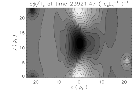
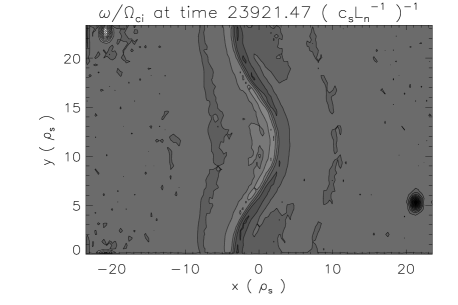
Figure 2: The normalised potential $e\phi/T_{e}$ and normalised vorticity $\omega/\Omega_{ci}$ at 23921.47 characteristic time units for the one stream. The minimum and maximum values of $e\phi/T_{e}$ are $\pm 0.019$ and the extrema for $\omega/\Omega_{ci}$ are -0.105 and 0.136. Maximum is white and minimum black in both plots. The vortices move in the negative $y$ direction at a speed of $0.2\max|v_{\star}|$.

Figure 3: Conservation of the generalised energy (dashed line) and enstrophy (dotted line) for the one stream. The change in generalised energy is $\bigtriangleup E/E_{0}=(E_{0}-E_{1})/E_{0}$ up to the end of the run and the change in generalised enstrophy is $\bigtriangleup U/U_{0}=(U_{0}-U_{1})/U_{0}$. The notation $E_{0}$ and $U_{0}$ is used for the initial values and $E_{1}$ and $U_{1}$ for the final values. Table 1 shows the conservation from times $0.48\times 10^{4}$ and $0.96\times 10^{4}$ $(c_{s}\max|L_{n}^{-1}|)^{-1}$ onwards.

	$\bigtriangleup E/E_{t}=(E_{t}-E_{1})/E_{t}$			$\bigtriangleup U/U_{t}=(U_{t}-U_{1})/U_{t}$
	$t=0.2$	$t=0.4$		$t=0.2$	$t=0.4$
One stream	$0.026$	$0.171$		$-0.048$	$-0.068$

Table 1: Conservation of the generalised energy $E$ and generalised enstrophy $U$ for the one stream. The time parameter $t$ is scaled such that $t=1$ is the end of the simulation.

In the statistical analysis, the higher moments of the distribution function may reveal important features of the statistics and the underlying dynamics of the process. Here, in the statistical analysis we will in addition consider the kurtosis and skewness. We define the kurtosis as the fourth moment divided by the square of the second moment $kurtosis=m_{4}/m_{2}^{2}$, note that sometimes $3$ is subtracted from the kurtosis yielding a zero kurtosis for a Gaussian distribution. A high value of the kurtosis is a key mark for a heavy tailed distribution which is flat at the centre. The skewness is defined as the third moment normalized by the $3/2$-power of the second moment, $skewness=m_{3}/m_{2}^{3/2}$ and describes the asymmetry of the PDF around its mean value.

In Figure 4, the kurtosis along the $x$ direction for the original time series is compared to the ARIMA modeled residual stochastic part of the time series. At some negative $x$ locations distributions with elevated tails are found in the potential for the original time traces however this behaviour is not found for the vorticity. Furthermore, comparing the kurtosis of the potential and vorticity of the ARIMA modeled time traces the region with elevated tails coincide, as an indication of Eq. (5).

Figure 5 displays the PDFs at several positions marked by black lines in Figure 4 along the $x$ direction. The time traces are normalized in order to be able to show several PDFs in the same graph according to $PDF(\tilde{\phi})=PDF[(\phi_{res}-\mu)/\mu]$, where $\mu$ is the mean value and $\phi_{res}$ is the residual after the ARIMA process. An analogous definition is adopted for the vorticity $\tilde{\omega}$. Here it can be seen that the PDFs of potential and kurtosis have exponential tails at the positions with higher kurtosis compared to the middle region which seems to exhibit Gaussian statistics. Note at some radial positions we find very large values of kurtosis signifying distributions with heavy tails and $\chi<1$. Moreover, the PDFs are nearly symmetric yielding small values of the skewness measure. In particular, Figure 2 shows that the time evolution of the electrostatic potential exhibits a structure of alternating negative and positive polarity vortices along the poloidal (or $y$) direction, indicating that the poloidal average for the nonlinear term is weak. At the same time the vortices are not symmetric about the $x=0$ axis and these asymmetries result in the vorticity-like statistics.

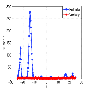
Figure 4: The kurtosis of the potential and vorticity time traces along the x direction in the one stream case are shown for the original time traces (graph on the left) compared to the ARIMA modeled time traces (graph on the right).

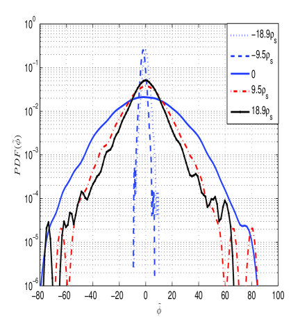
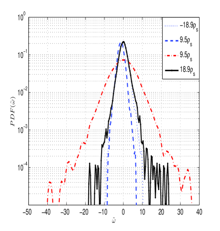
Figure 5: Numerical PDFs along the x direction of the potential (graph on the left) and vorticity (graph on the right) time traces in the one stream case. The various x positions sampled are indicated by black vertical lines in Figure 4.

IV.2 Two adjacent anti-parallel streams

The background density gradient (Figure 6) generates two streams flowing anti-parallel to each other with $\max|v_{\star}|$ centred at $x=\pm 3.5\rho_{s}$. The two streams flow adjacent to each other so that the edges of the streams are at $x=\pm 14\rho_{s}$ and $x=0$, where $v_{\star}$ becomes zero. Two cases with different $\max|v_{\star}|$ are studied: a slow-flowing and a fast-flowing system. For the slow-flowing streams the characteristic length and time give $\max|v_{\star}|=11.2\times 10^{4}$ cm s^-1. The fast-flowing streams have a $\max|v_{\star}|$ of 3.6 times that of the slow-flowing streams. Consequently the diamagnetic velocity gradient is larger for the fast-flowing streams.

As in the case of one stream (Section IV.1), the initialisation creates many vortices that merge to form monopolar vortices moving in each of the streams. In the case of the slow-flowing streams, a smaller gradient in the diamagnetic velocity shear exists between the two streams, compared to the shear in the case of the fast-flowing streams. As a result, there are more interactions between the vortices in the anti-parallel streams in the case of the slow-flowing streams. This manifests itself in Figure 7 by the fact that the two vortices situated inside the different streams move in the same direction, while the two vortices in Figure 8 move in opposite directions.

Positive vortices do not move in the direction of the stream where they are situated. Instead, they tend to move in the direction of the stream that is sampled by the edge of the vortex. This is clearly shown in Figures 7 and 8. The negative vortices are dragged in the direction of their neighbouring positive vortices, shown by the vortex at $x=0$ in Figure 7 and the one at $x=-11\rho_{s}$ in Figure 8. When the negative vortices are far enough from a positive vortex, their movement is determined by the flow direction sampled by their edge, as shown by the vortex at $x=15\rho_{s}$ in Figure 7. When vortices are far removed from the central flow streams and the vortices residing there, they exhibit small random movements, shown by the positive vortex at $x=-15\rho_{s}$ in Figure 7 and the negative vortex at $x=16\rho_{s}$ in Figure 8.

The generalised energy and enstrophy conservation follow the same pattern as for one stream (Section IV.1): after initialisation and large changes in energy and enstrophy the simulation produces a solution with less changes in these quantities. This is shown in Table 2 where the change measured from 40% of the duration to the end of the time-line is approximately half the change measured from 20% to the end. The energy and enstrophy change throughout the run as the two adjacent streams influence each other. There is less interaction between the two streams when the diamagnetic velocity gradient between them is larger. This manifests in slightly better conservation in the faster streams (Table 2).

Figure 6: Constant $x$ profile of diamagnetic velocity $v_{\star}$ normalised to $\max|v_{\star}|$ for two anti-parallel streams. For slow flows the characteristic time is $(c_{s}L_{n}^{-1})^{-1}=3.8\times 10^{-5}$ s and for fast flows it is $(c_{s}L_{n}^{-1})^{-1}=10^{-5}$ s.

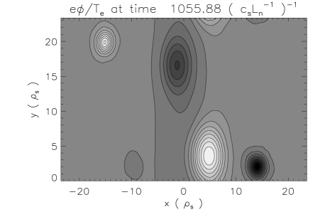
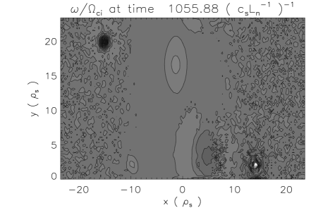
Figure 7: The normalised potential $e\phi/T_{e}$ and normalised vorticity $\omega/\Omega_{ci}$ at 1055.88 characteristic time units for the slow-flowing streams. The minimum and maximum values of $e\phi/T_{e}$ are $-1.7\times 10^{-2}$ and $1.4\times 10^{-2}$. The extrema for $\omega/\Omega_{ci}$ are $-9.3\times 10^{-2}$ and 0.13. Maximum is white and minimum black in both plots. The positive vortex at $x=5\rho_{s}$ moves in the negative $y$ direction at an approximate speed $3.4\max|v_{\star}|$, while the negative vortex at $x=0$ moves at approximate $2\max|v_{\star}|$ in the negative $y$ direction. It accelerates and decelerates every time the positive vortex passes it on its right hand side. The positive vortex at $x=-15\rho_{s}$ drifts slowly and randomly, while the negative vortex at $x=15\rho_{s}$ moves at speed $0.4\max|v_{\star}|$ in the positive $y$ direction.

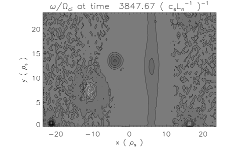
Figure 8: The normalised potential $e\phi/T_{e}$ and normalised vorticity $\omega/\Omega_{ci}$ at 3847.67 characteristic time units for the fast-flowing streams. The minimum and maximum values of $e\phi/T_{e}$ are $-1.8\times 10^{-2}$ and $10^{-2}$, while the extrema for $\omega/\Omega_{ci}$ are $-3.9\times 10^{-2}$ and 0.18. Maximum is white and minimum black in both plots. The negative vortex at $x=-11\rho_{s}$ moves at speed $0.9\max|v_{\star}|$ and the positive vortex at $x=-4\rho_{s}$ moves at $\max|v_{\star}|$, both in the positive $y$ direction. The positive vortex at $x=6\rho_{s}$ moves at speed $0.4\max|v_{\star}|$ in the negative $y$ direction while the negative vortex at $x=16\rho_{s}$ undergoes small and slow random movements.

	$\bigtriangleup E/E_{t}=(E_{t}-E_{1})/E_{t}$			$\bigtriangleup U/U_{t}=(U_{t}-U_{1})/U_{t}$
	$t=0.2$	$t=0.4$		$t=0.2$	$t=0.4$
Slow-flowing streams	$0.50$	$0.29$		$0.63$	$0.37$
Fast-flowing streams	$0.41$	$0.26$		$0.52$	$0.30$

Table 2: Conservation of the generalised energy $E$ and generalised enstrophy $U$ for two anti-parallel streams. The time parameter $t$ is scaled such that $t=1$ is the end of each simulation.

As a comparison to the statistical analysis of the one stream case, we will consider the time evolution of the stochastic part of the electrostatic potential and vorticity for both slow-flowing and fast-flowing anti-parallel streams. In Figure 9(a), the kurtosis of the potential and vorticity time traces are displayed corresponding to the simulation of the slow flow presented in Figure 7.

We find similarly good correspondence in kurtosis profiles between the potential and vorticity as was found in the case of one stream (Section IV.1) for the stochastic residual part whereas for the original time traces no such correspondence could be found. We have omitted the figures of the kurtosis of original time series due to space limitations here and in the rest of the paper, since these do not provide any additional useful information.

In Figure 10 and 11, the numerical PDFs of the stochastic part $\phi_{res}$ are shown for the CHM simulations of Figure 7. We find that at the edge of the stream the PDFs are close to Gaussian whereas at the stream centre other nonlinear features can be found. Here we will utilize Eq. (4) in the following cases: Laplacian distribution denotes the analytical model for $\chi=1.0$, whereas a Gaussian PDF is represented by $\chi=2.0$. The appearance of a Laplacian distribution at the stream (Figure 11) is suggestive of a vorticity conserving nonlinear system falcovich2011 ; anderson4 , whereas a Gaussian distribution is likely for a weakly nonlinear system anderson2 or dynamics impeded by a strong zonal flow anderson3 .

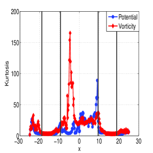
(a)                   (b)

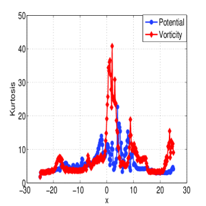
Figure 9: The kurtosis of the potential and vorticity of the ARIMA modeled time traces along the $x$ direction are shown for (a) the slow-flowing and (b) the fast-flowing anti-parallel cases.

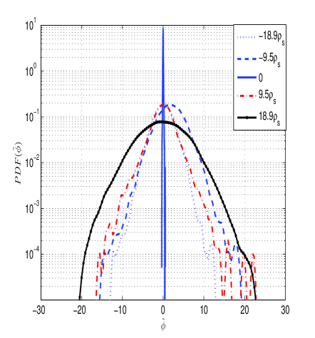
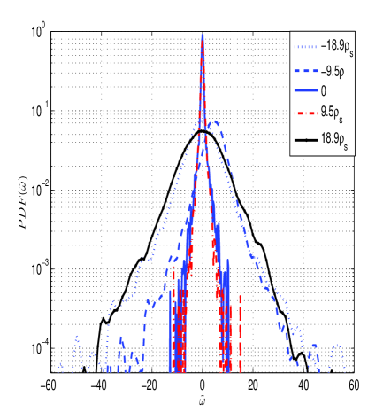
Figure 10: The PDFs of the potential (graph on left) and vorticity (graph on right) time traces along the $x$ direction in the slow-flowing anti-parallel case. The various $x$ positions sampled are indicated by black lines in Figure 9(a).

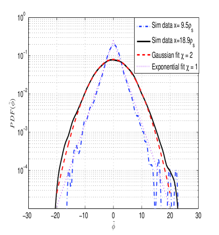
Figure 11: Fits to the two salient types of PDFs, the Gaussian and the Laplacian (exponential) distributions.

In Figure 9(b) the kurtosis of the time series generated by the fast-flowing anti-parallel streams corresponding to the simulation presented in Figure 8. The ARIMA modeled time trace of potential and vorticity follow each other reasonably well compared to the original time traces. Also here the skewness is small and the PDFs are Gaussian or exponential.

IV.3 Two streams with space between them

Figure 12 shows the background density gradient generating the two cases studied here: two streams flowing parallel to each other and two streams flowing anti-parallel to each other. For both cases there exists a space between the streams. The parallel streams are located at positions $x\in[-14,-4]$ and $x\in[4,14]$ with $\max|v_{\star}|$ at $x=\pm 9\rho_{s}$ and $v_{\star}=0$ outside these intervals. The anti-parallel streams are located at positions $x\in[-16,-6]$ and $x\in[6,16]$ with $\max|v_{\star}|$ at $x=\pm 11\rho_{s}$ and $v_{\star}=0$ outside these intervals. The characteristic length and time are the same in both cases, giving $\max|v_{\star}|=4.7\times 10^{4}$ cm s^-1.

Initial pairs of bipolar vortices merge to form monopolar vortices. In the case of two parallel flowing streams, all the vortices move in the flow direction of the two streams (Figure 13). These vortices exhibit the same behaviour as those in Section IV.2, namely they move in the direction of the flow sampled by their edges. Vortices outside the two streams are not influenced by the flow direction of the streams, e.g., the vortices at $x=\pm 20\rho_{s}$ in Figure 13.

In the case of the two anti-parallel flowing streams, monopolar vortices form inside the streams from bipolar vortices after initialisation. These vortices move in the opposite direction of the stream in which they reside. Monopolar vortices forming between the two anti-parallel streams at positions $x>0$ move in the flow direction their edges sample, i.e., the negative $y$ direction. At some stage during the simulation these vortices migrate in the negative $x$ direction, moving through the stream situated at $x=-10\rho_{s}$ and in the process destroying the vortices in that stream. The result is shown in Figure 14 where one vortex, situated at $x=-\rho_{s}$, moves between the streams in the negative $y$ direction while another moves in the opposite direction of the stream flow at $x=8\rho_{s}$.

Table 3 shows that the generalised energy conservation is good for the two streams flowing in the same direction, but bad for the anti-parallel streams. This shows that the amplitude of the fluctuations decrease more in the latter case. There is no discernible pattern in the conservation of the generalised enstrophy.

Figure 12: Constant $x$ profiles of diamagnetic velocity $v_{\star}$ normalised to $\max|v_{\star}|$ for two streams with a space between them. The characteristic time is $(c_{s}L_{n}^{-1})^{-1}=8.9\times 10^{-6}$ s for both parallel and anti-parallel streams.

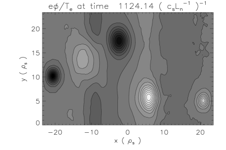
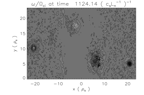
Figure 13: The normalised potential $e\phi/T_{e}$ and normalised vorticity $\omega/\Omega_{ci}$ at 1124.14 characteristic time units for two parallel streams. The minimum and maximum values of $e\phi/T_{e}$ are $-2.3\times 10^{-2}$ and $2.4\times 10^{-2}$, while the extrema for $\omega/\Omega_{ci}$ are 0.18 and 0.2. Maximum is white and minimum black in both plots. The negative vortex at $x=-3\rho_{s}$ moves at speed $0.7\max|v_{\star}|$ and the positive vortex at $x=6\rho_{s}$ moves at $1.2\max|v_{\star}|$, both in the negative $y$ direction.

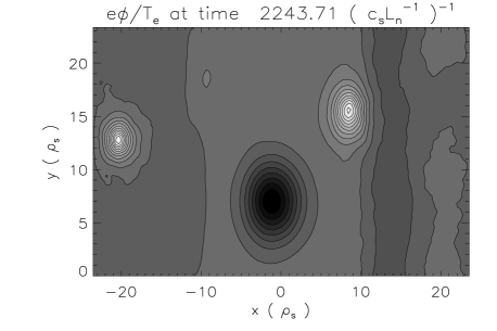
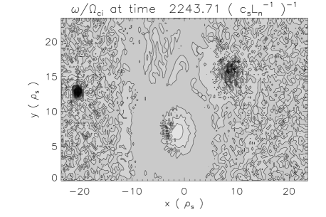
Figure 14: The normalised potential $e\phi/T_{e}$ and normalised vorticity $\omega/\Omega_{ci}$ at 2273.71 characteristic time units for anti-parallel streams. The minimum and maximum values of $e\phi/T_{e}$ are $-1.8\times 10^{-2}$ and $2.5\times 10^{-2}$, while the extrema for $\omega/\Omega_{ci}$ are -0.25 and $5.2\times 10^{-2}$. Maximum is white and minimum black in both plots. The negative vortex at $x=-\rho_{s}$ moves at speed $1.4\max|v_{\star}|$ in the negative $y$ direction and the positive vortex at $x=8\rho_{s}$ moves at speed $0.6\max|v_{\star}|$ in the positive $y$ direction. The positive vortex at $x=-21\rho_{s}$ hardly moves at all.

	$\bigtriangleup E/E_{t}=(E_{t}-E_{1})/E_{t}$			$\bigtriangleup U/U_{t}=(U_{t}-U_{1})/U_{t}$
	$t=0.2$	$t=0.4$		$t=0.2$	$t=0.4$
Parallel streams	$0.03$	$-0.003$		$0.007$	$-0.21$
Anti-parallel streams	$0.32$	$0.160$		$0.274$	$0.02$

Table 3: Conservation of the generalised energy $E$ and generalised enstrophy $U$ for two streams with a space between them. The time parameter $t$ is scaled such that $t=1$ is the end of each simulation.

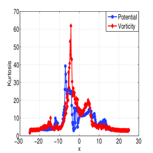
(a)                   (b)

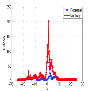
Figure 15: The kurtosis of the potential and vorticity of the ARIMA modeled time traces along the $x$ direction are shown in the (a) parallel and (b) anti-parallel cases.

Figure 15 presents the kurtosis generated with two imposed parallel or anti-parallel flows with a spacing between them. The statistics are obtained from the time evolution of the electrostatic potential in Figures 13 and 14 for the parallel and anti-parallel flows respectively. Note that the kurtosis of time traces of potential and vorticity follow each other reasonably well compared to the original time traces.

V Discussion and Summary

In this paper simulations of unforced Charney-Hasegawa-Mima (CHM) flows have been performed where we have imposed constant background density profiles on the CHM equation. In this manner we generated a single zonal flow, anti-parallel flows with slow and fast moving plasma adjacent to each other, as well as parallel and anti-parallel flows with a space between the flow streams.

In the single flow stream a chain of monopolar vortices form along the stream with their widths determined by the stream width and with polarities opposite from their neighbours. The vortex chain moves in the flow direction. When two anti-parallel zonal flows are placed adjacent to each other, monopolar vortices form in each stream but they are affected by the neighbouring stream and vortices in their close proximity. The smaller the flow velocity gradients are, the more interaction occurs. Vortices move in the direction their edges sample. In addition, negative polarity vortices in the presence of positive vortices are dragged along by the positive vortex. When two streams are placed a distance from each other, monopolar vortices form inside as well as between the streams. All vortices move in the flow direction when the streams flow in parallel. In the case of anti-parallel flow the vortex movement is in the opposite direction of the residing flow velocities. Vortex movement between the two flows are dictated by the flow direction the vortex edge samples.

After initialisation bipolar vortices form that merge and destroy each other until only monopolar vortices survive, which leads to enstrophy changes during the initial phase. The amplitudes of the vortices also change to a stable value during this phase, hence an initial change in energy. Once the initial phase is over, the energy and enstrophy conservation is good for the one stream. In the case of the two stream scenarios the energy and enstrophy are conserved to a lesser extent in some numerical runs and to a larger extent in others. This is because vortices keep on being created and destroyed as they interact in a random manner with each other and the sheared flow.

We have sampled time series at points in the radial direction (poloidally averaged) of the electrostatic potential and corresponding vorticity generated by the simulations. Our aim is to evaluate the intermittent characteristics of the time series by using a standard Box-Jenkins modeling. This mathematical procedure effectively removes deterministic autocorrelations from the time series, allowing for the statistical interpretation of the stochastic residual part. The numerically generated time traces are compared with predictions from a nonperturbative theory, the so-called instanton method for computing probability density functions (PDFs) in turbulence. More specifically the numerically generated time traces are analysed using the ARIMA model and fitted with analytical models accordingly. In the simulations presented here we find that an ARIMA(3,1,0) model presents an adequate description of the stochastic process.

The time series of the ARIMA modeled stochastic residual of cases described in section IV (A,B,C) of the potential and vorticity exhibit in general a uni-modal PDF with Gaussian features or a PDF with exponential tails. In summary, the PDF $\sim\exp\big{(}-const\ |\phi|^{\chi}\big{)}$ with $\chi=2.0$ or exponential statistics are found with ($\chi=1.0$). The different configurations are represented by an imposed slow and a fast zonal flow as well as parallel and anti-parallel flows. The rationale for using the ARIMA model is to uncover the stochastic process hidden in the numerically generated time trace. The ARIMA process is specifically designed to identify correlations in a time trace by utilizing a differencing procedure and thus provides us with an efficient model how to subtract the correlations in time from the full signal. The objective of this work is to identify the particular stochastic process that is generating the time trace. The one important restriction of this procedure is that the stochastic process has to be stationary with respect to the mean and variance. For an arbitrary stochastic process, there exist formal tests to check whether stationarity holds. In this particular example of CHM zonal flows with a constant background density profile generating the process, this is fulfilled except for a short interval at the start of the simulation.

One non-trivial aspect of the statistics of the electrostatic potential in the CHM system is conservation of energy and enstrophy that may lead to a Gibbsian equilibrium distribution. However with the imposed shear flow through the varying density gradient, non-vanishing triad interactions redistribute energy between the modes, contributing to a situation where the PDFs deviate from the Gaussian form at some radial locations. For a general discussion see Krommeskrommes_kinetic . The cascade processes or redistribution energy and enstrophy can also be directly seen in the simulations as deviations in the conserved quantities.

To this end, in general we find an emergent universal exponential scaling of the distribution functions (Laplace distribution with $\chi=1.0$) that accurately describes the statistics of the time series of the electric potential and vorticity. Analysing the profiles along the $x$ coordinate of the kurtosis of the potential and vorticity time series we find striking similarity suggestive of the relation in Eq. (5). Exceptions to the named distributions occur where strong nonlinear interactions are present in the dynamics where the PDFs are sub-exponential with $\chi<1.0$ and high values of the normalized fourth moment (kurtosis) is found.

References

- (1) S. Zweben, J. A. Boedo, O. Grulke, C. Hidalgo, B. LaBombard, R. J. Maqueda, P. Scarin and J. L. Terry, Plasma Phys. Contr. Fusion 49, S1 (2007)
- (2) P. A. Politzer, Phys. Rev. Lett. 84, 1192 (2000)
- (3) P. Beyer, S. Benkadda, X. Garbet and P. H. Diamond, Phys. Rev. Lett. 85, 4892 (2000)
- (4) J. F. Drake, P. N. Guzdar and A. B. Hassam, Phys. Rev. Lett. 61, 2205 (1988)
- (5) G. Y. Antar, S. I. Krasheninnikov, P. Devynck, R. P. Doerner, E. M. Hollman, J. A. Boedo, S. C. Luckhardt and R. W. Conn, Phys. Rev. Lett. 87, 065001 (2001)
- (6) B. A. Carreras, C. Hidalgo, E. Sanchez, M. A. Pedrosa, R. Balbin, I. Garcia-Cortes, B. van Milligen. D. E. Newman and V. E. Lynch, Phys. Plasmas 3(7), 1996
- (7) Nagashima, S.-I. Itoh, S. Inagaki, H. Arakawa, N. Kasuya, A. Fujisawa, K. Kamataki, T. Yamada, S. Shinohara, S. Oldenbürger, M. Yagi, Y. Takase, P. H. Diamond and K. Itoh, Phys. Plasmas 18, 070701 (2011)
- (8) G. Dif-Pradalier, P. H. Diamond, V. Grandgirard, Y. Sarazin, J. Abitebboul, X. Garbet, Ph. Ghendrih, A. Strugarek, S. ku and C. S. Chang, Phys. Rev. E 82, 025401 (2010)
- (9) P. H. Diamond, S.-I. Itoh, K. Itoh and T. S. Hahn, Plasma Phys. Contr. Fusion 47, R35 (2005)
- (10) P. H. Diamond, A. Hasegawa and K. Mima, Plasma Phys. Contr. Fusion 53, 124001 (2011)
- (11) J. W. Connor, T. Fukuda, X. Garbet, C. Gormezano, V. Mukhovatov, M. Wakatani, the ITB Database Group and the ITPA Topical Group on Transport and Internal Barrier Physics, Nucl. Fusion 44, R1 (2004)
- (12) K. Itoh, S.-I. Itoh, P. H. Diamond, T. S. Hahn, A. Fujisawa, G. R. Tynan, M. Yagi and Y. Nagashima, Phys. Plasmas 13, 055502 (2006)
- (13) J. W. Connor and T. J. Martin, Plasma Phys. Contr. Fusion 49, 1497 (2007)
- (14) A.-S. Smedman, U. Högstroöm and J. C. R. Hunt, Q. J. R. Meteorol. Soc. 130, 31 (2004)
- (15) T. V. Prabha, M. Y. Leclerc, A. Karipot, D. Y. Hollinger and E. Mursch-Radlgruber, Boundary-Layer Meteorol. 126 219 (2008)
- (16) H. F. Duarte, M. Y. Leclerc, G. Zhang, Theor. Appl. Climatol. 110 359 (2012)
- (17) W. Horton and Y.-H. Ichikawa, Chaos and Structures in Nonlinear Plasmas (World Scientific, Singapore, 1996), Sections 6.1 & 6.2, p.221
- (18) B. A. Carreras, K. Sidikman, P. H. Diamond, P. W. Terry and L. Garcia, Phys. Fluids B 4, 3115 (1992)
- (19) X. Garbet, Y. Sarazin and P. Ghendrih, Phys. Plasmas 9, 3893 (2002)
- (20) G. R. Tynan, C. Holland, J. H. Yu, A. James, D. Nishijima, M. Shimada and N. Taheri, Plasma Phys. Contr. Fusion 48, S51 (2006)
- (21) C. Connaughton, S. Nazarenko and B. Quinn, EPL 96, 25001 (2011)
- (22) J. G. Charney, Geofys. Publ. Kosjones Norsk Videnskap. Akad. Oslo, 17(2) 1-17 (1948)
- (23) A. Hasegawa and K. Mima, Phys. Rev. Lett. 39, 205 (1977)
- (24) A. Hasegawa and K. Mima, Phys. Fluids, 21, 87 (1978)
- (25) G. J. J. Botha, M. G. Haines and R. J. Hastie, Phys. Plasmas 6, 3838 (1999)
- (26) J. Nycander, J. Plasma Physics 39, 413 (1988)
- (27) W. Horton, Rev. Mod. Phys. 71, 735 (1999)
- (28) A. Hasegawa, C. G. Maclennan and Y. Kodama, Phys. Fluids, 22, 2122 (1979)
- (29) A. Arakawa, J. Comp. Physics 1, 119 (1966)
- (30) G. Box, G. Jenkins, G. Reinsel, Time series analysis; Forecasting and control, (Prentince Hall, 1994)
- (31) J. Zinn-Justin, Field Theory and Critical Phenomena (Clarendon, Oxford, 1989)
- (32) V. Gurarie and A. Migdal, Phys. Rev. E 54, 4908 (1996)
- (33) G. Falkovich, I. Kolokolov, V. Lebedev and A. Migdal, Phys. Rev. E 54, 4896 (1996)
- (34) E. Kim and P. H. Diamond, Phys. Rev. Lett. 88, 225002 (2002)
- (35) J. Anderson and E. Kim, Phys. Plasmas 15, 082312 (2008)
- (36) E. Kim and J. Anderson, Phys. Plasmas 15, 114506 (2008)
- (37) J. Anderson and P. Xanthopoulos, Phys. Plasmas 17, 110702 (2010)
- (38) G. Falcovich and V. Lebedev, Phys. Rev. E 83, 045301 (2011)
- (39) J. Anderson and E. Kim, Nucl. Fusion 49, 075027 (2009)
- (40) J. Anderson, F. D. Halpern, P. Xanthopoulos, P. Ricci and I. Furno, Phys. Plasmas 21, 122306 (2014)
- (41) J. A. Krommes, Phys. Reports, 360 1-352 (2002), See Section 3.7.2.