Statistics of Chaotic Resonances in an Optical Microcavity

Abstract

Distributions of eigenmodes are widely concerned in both bounded and open systems. In the realm of chaos, counting resonances can characterize the underlying dynamics (regular vs. chaotic), and is often instrumental to identify classical-to-quantum correspondence. Here, we study, both theoretically and experimentally, the statistics of chaotic resonances in an optical microcavity with a mixed phase space of both regular and chaotic dynamics. Information on the number of chaotic modes is extracted by counting regular modes, which couple to the former via dynamical tunneling. The experimental data are in agreement with a known semiclassical prediction for the dependence of the number of chaotic resonances on the number of open channels, while they deviate significantly from a purely random-matrix-theory-based treatment, in general. We ascribe this result to the ballistic decay of the rays, which occurs within Ehrenfest time, and importantly, within the timescale of transient chaos. The present approach may provide a general tool for the statistical analysis of chaotic resonances in open systems.

Introduction. The statistics of chaotic resonances has been a central topic of theoretical and experimental interest for decades Wirzba ; folk96 ; ElastRes96 ; Weidenm ; ColdAtomRes ; CondMatRes ; CaoWier ; PLS00 , as a doorway to better understand chaotic scattering in quantum mechanics BR ; Gasp89 ; Anlage ; squid . Counting chaotic resonances notably finds applications in optical resonators Star00 ; Hack05 ; SWM , where chaos can be used, for example, to enhance energy storage storage13 or enhance coupling Yang_dyntun ; xiao13 . In the realm of fundamental problems, an estimate of the number of states within a certain frequency interval is given by the fractal Weyl law LSZ ; ketzWeyl ; IShudoSchom ; Zwor_pre ; Zwor_prl . Predicted more than a decade ago, this theory is still awaiting experimental confirmation at optical frequencies. The delay is mainly due to two obstacles: (i) the theoretical problem of accounting for partial absorption Nonnenmacher ; Schonwetter ; and (ii) the experimental challenge of analyzing overlapping resonances WierMain . By introducing methods to overcome these hurdles, we theoretically and experimentally study the statistics of chaotic resonances in two-dimensional asymmetric optical microcavities, and thus present a significant result in the context of fractal Weyl laws at optical frequencies. An absorber is placed underneath the microcavity appositely to realize a virtually full opening, and therefore solve the problem of partial absorption. In order to handle overlapping resonances, we exploit the mixed classical phase space of the present cavity, and exclusively count high-$Q$ regular modes, easily recognized in the measured spectra due to their narrow linewidths, and that enables us to draw information on the low-$Q$ chaotic modes, coupled to the regular ones via dynamical tunneling davis81 .

Figure 1: (color online) (a) Sketch of the deformed microcavity with an inner absorber, characterized by the angle $\theta_{a}$. (b) Poincaré surface of section of the microcavity ($\hat{\phi}\equiv\phi/2\pi$) with deformation factor $\eta=11.7\%$. Blue orbits at the top are regular, black ones are chaotic. The red solid line indicates the angle of total internal reflection, while the dashed curve is given by an absorption angle such that $r\simeq 0.77$. Different shades of color indicate loss to the absorber (lighter) and by refraction into air (darker). (c) Schematic representation of the free-space coupled cavity system. (d) A typical transmission spectrum with the high-$Q$ regular modes highlighted.

Theoretical model. The dynamics inside the cavity is described by a non-Hermitian Hamiltonian $H=H_{0}+V$, where $H_{0}$ has eigenstates $|C_{\omega}\rangle$ (regular) and $|C_{n}\rangle$ (chaotic), while $V$ represents the coupling between them BTU ; Backer1 . Following a standard approach Fano ; AnYang , the electromagnetic field excited by the incident beam can be written as a superposition of one regular and several chaotic modes, $\psi(x,t)=a_{\omega}(t)c_{\omega}(x)e^{-i\omega t}+\sum_{n}b_{n}(t)c_{n}(x)e^{-i\omega_{n}t}$. The $a_{\omega}$ and $b_{n}$ are oscillator amplitudes driven by the laser beam, coupled to each other with strength $V_{n}$ (real), with damping rates $\gamma_{\omega}$ and $\gamma_{n}$, respectively. Then, in the overdamped regime ($|V_{n}|\ll\gamma_{n}$), the dynamical equations for the time-dependent envelopes take the form Yang_dyntun

$$\dot{b}_{n}+\gamma_{n}b_{n} =f_{n}E_{0}-V_{n}a_{\omega},$$ (1a)

$$\dot{a}_{\omega}+\left[\gamma_{\omega}+i(\omega_{0}-\omega)\right]a_{\omega} ={\textstyle\sum\limits_{n}}V_{n}b_{n},$$ (1b)

where $f_{n}$ is the coupling strength of the $n$-th chaotic mode with the laser beam of amplitude $E_{0}$ and frequency $\omega_{0}$. We are interested in the steady-state solution, obtained by setting $\dot{a}_{\omega}=\dot{b}_{n}=0$. The amplitude $a_{\omega}$ of the envelope of the regular mode is then found to be

$$a_{\omega}=\frac{E_{0}\sum\limits_{n}f_{n}\frac{V_{n}}{\gamma_{n}}}{\left[\gamma_{\omega}+i(\omega-\omega_{0})\right]+\sum\limits_{n}\frac{V_{n}^{2}}{\gamma_{n}}}.$$ (2)

We only sum over $n_{\gamma}$ chaotic modes with linewidth smaller than a certain value set by $\gamma$, and use the averages $\bar{f},\bar{V},\bar{\gamma}$ to approximate the summations as ${\textstyle\sum_{n}}f_{n}\frac{V_{n}}{\gamma_{n}}\sim n_{\gamma}\frac{\bar{f}\bar{V}}{\bar{\gamma}},{\textstyle\sum_{n}}\frac{V_{n}^{2}}{\gamma_{n}}\sim n_{\gamma}\frac{\bar{V}^{2}}{\bar{\gamma}}$ SI . The result is, at resonance ($\omega=\omega_{0}$),

$$|a_{\omega}|^{2}=\epsilon^{2}\frac{n_{\gamma}^{2}}{\Gamma^{2}+n_{\gamma}^{2}},$$ (3)

where $\epsilon=E_{0}\bar{f}/\bar{V}$, and $\Gamma=\gamma_{\omega}\bar{\gamma}/\bar{V}^{2}$.

Equation (16) is central to the present work, as it bridges between the number of excited regular modes (proportional to $|a_{\omega}|^{2}$), which we measure directly, and the number of chaotic modes $n_{\gamma}$, which we estimate. In the spirit of Weyl law, we test the prediction SchomTwor

$$n_{\gamma,\mathrm{Weyl}}=MN^{-1/\mu\tau_{d}}\left[1-\frac{1}{\tau_{d}}\frac{1}{1-e^{-\gamma}}\right],$$ (4)

for the dependence of $n_{\gamma}$ on the number of open channels $N$. Here $M$ is the total number of chaotic states, $\tau_{d}=M/N$ is the mean dwelling time of a ray in the cavity, and $\mu$ is of the order of the Lyapunov exponent of the chaotic dynamics SI . We focus on the role of the prefactor $N^{-1/\mu\tau_{d}}$, which accounts for the instantaneous-decay modes escaping from the system within the Ehrenfest time of quantum-to-classical correspondence SchomJacq . By removing the prefactor, the remainder of Eq. (4) is solely based on random matrix theory (RMT) ZycSom , and will also be tested against the observations.

Absorber in the optical cavity. In order to achieve the full opening required to test these predictions, we introduce an absorber in the cavity. In the analysis, the dielectric microcavity [Fig. 1(a)] has the deformed circle $\rho(\phi)$ as boundary SI , and encloses an absorber of shape $\rho(\phi)-R$. Figure 1(b) shows the classical phase space, together with the critical line of total internal reflection ($\sin\theta_{c}$), as well as the line given by the incidence angle $\theta_{a}$, below which the reflected ray hits the absorber ThetaNote . We assume that the rays hitting the absorber are completely absorbed. The rays that escape the cavity by refraction into the air with an angle of incidence $\theta\ll\theta_{c}$ are very lossy, and, as such, they are not expected to contribute to the excitation of the regular modes, consistently with Eqs. (14) and (16).

For that reason, we only take into account the states supported on a strip of the chaotic phase space with momentum above a certain threshold, $\sin\theta>\sin\theta_{\mathrm{th}}$, to be chosen below but close enough to the critical line of total internal reflection. Let us introduce the notation $\xi\equiv\sin\theta_{a}-\sin\theta_{\mathrm{th}}$ to indicate the strip of the phase space opened by the absorber. Using the picture of Ref. SchomTwor , there are effectively $N$ open channels out of the $M$ Planck cells available in the phase space, produced by the absorber (full opening, $N_{a}$) and the refraction out of the cavity (partial opening, $N_{r}$), so that the mean dwelling time of a ray is given by

$$\tau_{d}=\frac{M}{N_{a}+N_{r}},$$ (5)

with $N_{r}=\frac{M}{A}\int_{\sin\theta_{a}}^{\sin\theta_{c}}d\sin\theta T(\sin\theta)$, $T$ transmission coefficient according to Fresnel law, and $A$ area of the phase space in exam, while $N_{a}=M\xi/A$.

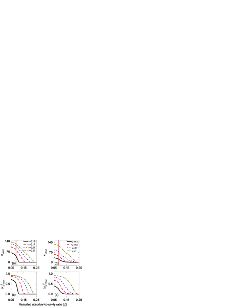
Figure 2: (color online) (a), (b) Number of chaotic states $n_{\gamma}$ vs. the rescaled absorber-to-cavity ratio $\xi$, obtained by RMT and Weyl law, respectively. (c), (d) The corresponding expectations for $|a_{\omega}|^{2}$. In (d), the smaller $\mu$, the more visible the tail of the excitation probability. The red vertical line corresponds to the critical angle, $\sin\theta_{c}\simeq 0.69$. Here $\sin\theta_{\mathrm{th}}=0.6$.

Recalling the original purpose of studying the statistics of chaotic resonances, we proceed by steps and first examine the RMT-based prediction $n_{\gamma,RMT}=M\left[1-\frac{1}{\tau_{d}}\frac{1}{1-e^{-\gamma}}\right]$, rewritten as (set $\hat{\xi}=1/\tau_{d}=\xi/A+N_{r}/M$)

$$n_{\gamma,RMT}=M\left[1-\frac{\hat{\xi}}{1-e^{-\gamma}}\right].$$ (6)

The theoretical expectation is portrayed in Fig. 2(a): $n_{\gamma,\mathrm{RMT}}$ changes relatively slowly for $\xi$ small such that $\theta_{a}<\theta_{c}$, when the loss is mainly due to refraction into air. Otherwise $n_{\gamma,\mathrm{RMT}}$ decreases more rapidly and linearly with $\xi$ in the region of total internal reflection, when the loss is entirely due to the absorber. Plugging Eq. (6) into Eq. (16), the probability of excitation of the high-$Q$ regular modes $|a_{\omega}|^{2}_{\mathrm{RMT}}$ starts to fall off as $\xi$ reaches some critical value, controlled by the parameter $\gamma$ [Fig. 2(c)]. The other parameter $\tilde{\Gamma}=\gamma_{\omega}\bar{\gamma}/M\bar{V}^{2}$ controls the slope of the curve. It is noted that the probability of excitation of the regular modes decreases dramatically when the loss is entirely due to the absorber, in which case the system is fully open.

On the other hand, the semiclassical estimate (4) becomes, as a function of $\hat{\xi}$,

$$n_{\gamma,\mathrm{Weyl}}=\frac{M^{1-\hat{\xi}/\mu}}{\hat{\xi}^{\hat{\xi}/\mu}}\left[1-\frac{\hat{\xi}}{1-e^{-\gamma}}\right].$$ (7)

The quantity $\mu$, of the order of the Lyapunov exponent of the chaotic region of the phase space SI , is what really characterizes (7), which resembles the linear RMT prediction (6) for large enough $\mu$, and otherwise becomes visibly nonlinear [Figs. 2(a) and 2(b)] when $\mu\ll 1$. This nonlinearity produces a characteristic tail in the curve expressed by Eq. (16) [Fig. 2(d)], meaning that the effect of the Ehrenfest time scale on the excitation of the regular modes is most evident slightly above the onset of chaos.

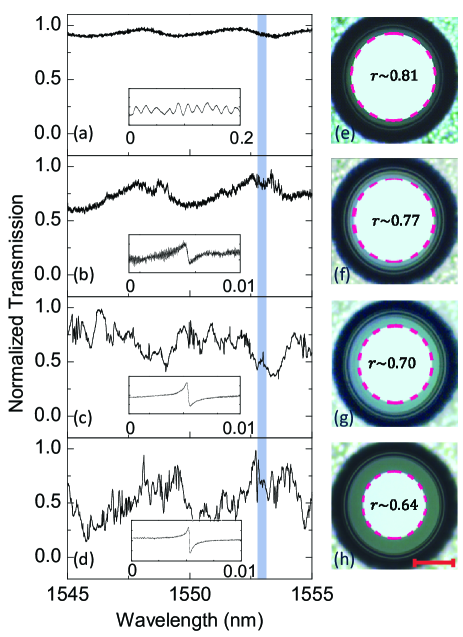
Figure 3: (color online) Normalized transmission and top-view optical images of the cavity with $r\simeq 0.81$ [(a) and (e)], $0.77$ [(b) and (f)], $0.70$ [(c) and (g)], and $0.64$ [(d) and (h)]. Inset of (a) shows background noise. Insets of (b)-(d) show the high-$Q$ modes. Reflection of the silica-to-silicon interface results in a brighter color for the silicon pillar in the optical image (boundary shown by red dashed curves). Scale bar is $50$ $\mathrm{\mu}$m.

Experimental setup and measurement. The experimental apparatus consists of a deformed toroidal microcavity xiao13 coupled to a laser beam (of wavelength $\lambda\simeq 1550$ or $635$ nm), as shown in Fig. 1(c). The microtoroid (refractive index $\simeq 1.44,1.46$ depending on $\lambda$) has principal (minor) diameters of $120$ $\mathrm{\mu}$m($5$ $\mathrm{\mu}$m), consistently with the two-dimensional model SI . Thus the effective Planck constant $h_{\mathrm{eff}}\sim\lambda/a\sim 10^{-2}$ ($a$: principal diameter) justifies the semiclassical analysis. The microcavity is fabricated through optical lithography, buffered HF wet etching, XeF2 gas etching, and CO2 pulse laser irradiation. The resulting silica microtoroid is supported by a silicon pillar of similar shape, which has a high refractive index ($\simeq 3.48,3.88$), and it acts as the absorber in the model. After each measurement of the free-space transmission spectrum [Fig. 1(d)], the top diameter of the silicon pillar, connected with the silica disk, is progressively reduced by a new isotropic XeF2 dry etching process. In this way we control the openness of the microcavity with the ratio $r$ between the top diameters of pillar and toroid. Finite element method simulations show that the light power decreases to less than $5\%$ of the input value, when propagating by a distance of $20$ $\mathrm{\mu}$m inside the $2$-$\mathrm{\mu}$m-thick silica waveguide bonding with a silicon wafer SI , as is reasonable to expect, given the high refractive index of the silicon. Thus the silicon pillar acts as a full absorber, consistently with the present model. On the other hand, high-$Q$ regular modes living inside the toroidal part, whose cross section has minor diameter of $5$ $\mathrm{\mu}$m, do not leak into the silicon pillar and therefore are not directly affected by the pillar size SI . The dependence of the free-space transmission spectra on the pillar size is shown in Fig. 3. When the pillar approaches the inner edge of the toroid [Figs. 3(a) and 3(e), $r\simeq 0.81$], no high-$Q$ regular modes are observed in the spectrum, since most of the probe laser field in the cavity radiates into the silicon and cannot tunnel to high-$Q$ regular modes. As we gradually reduce the size of the pillar [Fig. 3(f), $r\simeq 0.77$], increasingly many high-$Q$ modes appear in the spectrum [Fig. 3(b)]. When the absorber-to-cavity ratio $r$ is small enough [Figs. 3(g) and 3(h), $r\lesssim 0.7$], the transmission no longer changes sensibly [Figs. 3(c) and 3(d)], and the number of high-$Q$ modes in the spectrum also stabilizes.

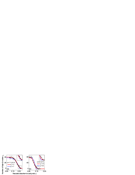
Figure 4: (color online) (a), (b) Number of high-$Q$ regular modes ($n_{\omega}$) observed experimentally in the microcavities of $\eta=11.7\%$, $6\%$ respectively, vs. rescaled absorber-to-cavity ratio $\xi$. Blue dashed and red solid curves are respectively RMT and Weyl-law best fits, whose goodness is assessed by $\chi^{2}$. Here $\sin\theta_{c}\simeq 0.69$ and $\sin\theta_{\mathrm{th}}=0.6$. Inset: area where the two curves differ most.

Statistics of chaotic resonances. As anticipated, we use the transmission spectra to test the theory, by counting the excited high-$Q$ regular modes for different sizes of the silicon pillar Note . The results are illustrated in Fig. 4, for two microcavities of distinct deformations. In the RMT-based approach [Eqs. (16) and (6)] we have two fitting parameters, $\gamma$ and $\tilde{\Gamma}$, while the total number of chaotic states is estimated theoretically as $M\simeq A/h_{\mathrm{eff}}$ ($A$ area of the phase space we consider). Figure 4(a) shows overall agreement between the experimental data (dots) and this theory (blue dashed curve), which however deviates from the tail visible at larger sizes of the absorber. The discrepancy becomes more apparent for the cavity with a lower deformation factor $\eta$ [Fig. 4(b)]. A quantitative test of the goodness of the fit yields a reduced $\chi^{2}\simeq 1.7,5.6$ for $\eta\simeq 11.7\%,6\%$ respectively chi-s ; SI , the latter deviating significantly from the optimal value of unity. The fitted maximum escape rate $\gamma\simeq 0.2,0.3$ is the inverse (in units of Poincaré time) of the minimum escape time $\tau_{esc}$ of the chaotic rays contributing to the excitation of the regular modes, from which $Q=2\pi\nu\tau_{esc}\sim 10^{3}$, on average ($\nu$ is the frequency of the laser beam). We find this estimate consistent with the typical order of $Q$ independently obtained from ray-dynamics simulations SI , which suggests the fitted parameter makes physical sense.

Next, we test the semiclassical correction (7), using the finite time Lyapunov exponent $\mu$ evaluated by direct iteration finLyap ; SI , with the estimated parameter $M$ and the fitted parameters $\gamma$ and $\Gamma$. It is found that the semiclassical correction (red solid curves) fits the experimental data better than the RMT-based estimate, especially at the smaller deformation, where the two predictions differ the most due to the smaller $\mu$ [cf. Fig. 2]. Here $\chi^{2}\simeq 1.3,1$, indicating good agreement. In particular, we are now able to account for the tail of the curve, which corresponds to the microcavity having the largest openings and thus with the maximum number of instantaneous decay states, where the semiclassical correction is decisive. More experimental and fitting results at different wavelengths and deformations support the above explanation SI .

Conclusion and discussion. Let us summarize the work done and the results obtained. By counting the high-$Q$ regular modes excited via dynamical tunneling as a function of the number of open channels, we have studied the statistics of the chaotic resonances in a dielectric microcavity with a full absorber.

As main result, the experimental data deviate from a purely RMT-based prediction, while they exhibit better agreement with a semiclassical expression that factors out the number of instantaneous decay modes. Importantly, the latter estimate depends on the Lyapunov exponent of the chaotic dynamics, and it accounts for a characteristic tail in the decay of the number of regular modes, which we interpret as a signature of the ballistic escape of the rays into the absorber, occurring within Ehrenfest time.

Although the theoretical analysis does not take into account either partial transport barriers MeissPBs ; KetzPBs , or the ”sticky” dynamics at the regular-chaotic border ketzWeyl ; IShudoSchom , which all cause long-time correlations to decay algebraically rather than exponentially, we argue in what follows that the current model is suitable for the resolution of our experiment. Figure 5 illustrates the survival probability in the chaotic region, obtained from extensive ray-dynamics simulations of the microcavity-shaped billiard: despite an overall power-law decay, a closer look at the short-time dynamics reveals that the decay is initially exponential, behavior known as transient chaos LaiTel .

The estimates for the dwelling time $\tau_{d}$, and the fitted value from the data of $\gamma$, maximum decay rate of the chaotic resonances, are both within the timescale of exponential decay. That suggests that the suppression by the absorber of the longest-lived resonances (that scale algebraically with $\gamma$ IShudoSchom ) alone does not affect the number of excited WGMs measured in the experiment, and therefore is not detected by the current apparatus.

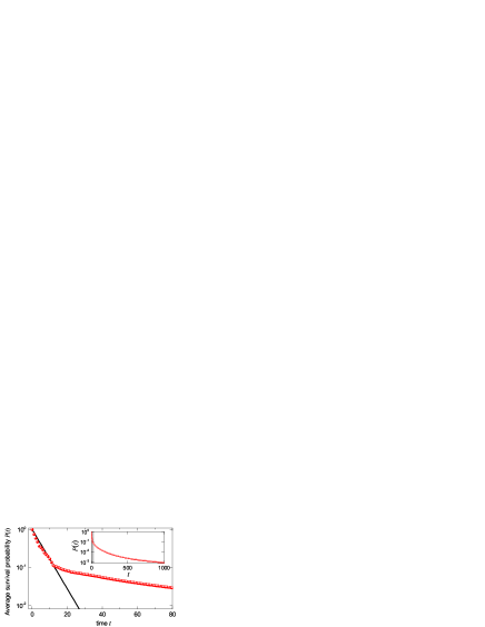
Figure 5: (color online) Survival probability in the chaotic region (logarithmic scale). Points: average survival probability $P(t)$ of a ray in the microcavity vs. $t$ (in units of Poincaré time) at $\eta=11.7\%,\xi=0.13$, from $10^{6}$ randomly-started trajectories. Line: $P(t)=\mathrm{exp}(-t/\tau_{d})$, $\tau_{d}=6$. Inset: the long-time simulation showing algebraic decay.

Acknowledgments— This project was supported by the 973 program (Grant No. 2013CB921904 and No. 2013CB328704) and the NSFC (Grants No. 61435001 and No. 11474011). D.L. acknowledges support from NSFC (Grant No. 11450110057-041323001). Z.-Y.L. was supported by the National Fund for Fostering Talents of Basic Science (Grant No. J1103205). L.W. fabricated the microcavities and performed measurements and numerical simulations. D.L. developed the theoretical model. Y.-F.X. supervised and coordinated the project. All authors contributed to the discussions and wrote the manuscript.

Supplemental Information to ‘Statistics of chaotic resonances in an optical microcavity’  

This Supplementary Material is organized as follows. In Sec. I, we describe the boundary shape of the cavity and its unidirectional emission. In Sec. II, the $Q$ factor magnitude distribution of the chaotic rays is estimated by ray-dynamics simulation. In Sec. III, we show geometry and field distribution of microtoroid by SEM images and finite element method modeling. In Sec. IV, power loss in the silica waveguide bonding with a thick silicon layer is studied. In Sec. V, we provide a cross-check that many high-$Q$ modes do exist in the deformed microcavity by exciting them directly through a tapered fiber. In Sec.VI, the process of obtaining the number of high-$Q$ regular modes is described. Sec. VII deals with the definition of the Ehrenfest time and rescaling of Lyapunov exponent in the Wey law. In Sec. VIII, we explain the $\chi^{2}$ test used to assess the goodness of our fits. In Sec. IX, more experimental and fitting results are shown. Sec. X contains tables with the quantities and parameters used in our final results. In Sec. XI, the phase space with a small deformation factor together with the survival probability of a ray in the chaotic region are shown. In Sec. XII, we study the relation between the decay rates of WGMs and their coupling to chaotic modes.

I Boundary shape of the cavity

The deformed microtoroid cavity in our experiment has a boundary shape given by the curve

$$\rho(\phi)=\left\{\begin{array}[c]{cc}\rho_{0}(1+\epsilon\sum_{i=2,3}a_{i}\cos^{i}\phi)&\mathrm{for}\cos\phi\geq 0,\\ \rho_{0}(1+\epsilon\sum_{i=2,3}b_{i}\cos^{i}\phi)&\mathrm{for}\cos\phi<0,\end{array}\right.$$ (1)

with $a_{2}=-0.1329,a_{3}=0.0948,b_{2}=-0.0642$, and $b_{3}=-0.0224$. The WGMs in the deformed microcavity have been demonstrated to possess ultrahigh quality factors in excess of $10^{8}$ in the $1550$ nm wavelength band and to exhibit highly directional emission towards the $180^{\circ}$ far-field direction, which emits tangentially along the cavity boundaries at polar angles $\phi=\pi/2$ and $\phi=3\pi/2$. The deformation is controlled by $\eta=(d_{\max}-d_{\min})/d_{\max}$, $d_{\max}$ and $d_{\min}$, respectively, the maximum and minimum diameters of the cavity. The parameter $\eta$ is related to $\epsilon$ through $\eta=\epsilon\left|a_{2}+a_{3}+b_{2}-b_{3}\right|/2$. The $\eta$ of cavity shape we used to draw the Poincaré surface of section in the main text is $11.7\%$.

II Estimating the $Q$ factor magnitude distribution of the chaotic rays

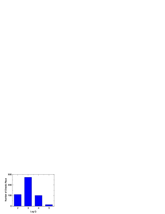
Figure 1: Statistics of the quality factor for the chaotic rays in the deformed microcavity, from a ray-dynamics simulation.

A ray-dynamics simulation is performed on the billiard with boundary set by Eq. 1 ($\epsilon$=1). A swarm of initial points, randomly chosen in the chaotic region of the phase space, is iterated $1000$ times. Each ray is considered to have escaped when it falls below the critical line of total internal reflection, and its quality factor $Q$ is measured as $Q=2\pi\tau\nu$, with $\tau$ lifetime of the ray and $\nu$ frequency of the light. The statistics shown in Fig. 1 indicates that $Q$ is mostly of the order of $10^{3}$, confirming the estimation from the experimental results.

III Geometry and field distribution of the microtoroid

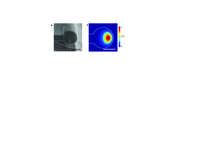
Figure 2: (a) SEM cross-section image of the microtoroid. It is an oblique view taken by an angle of $56^{\circ}$ with the horizontal direction. (b) COMSOL Multiphysics finite element method modeling of a fundamental TE mode. The white solid curve is the boundary of the cavity. The scale bar is 3 $\mathrm{\mu}$m.

The field localized at the boundary of the cavity (WGM) is shown in Fig. 2 (toroidal section). It can be seen that the toroid has little influence on the propagation of chaotic light fields into the disk part of the cavity since the optical WGMs mainly locate at the same plane with the disk. This observation supports our two-dimensional model of the microcavity.

IV Power loss in the silica waveguide bonding with a thick silicon layer

The finite-element simulation in Fig. 3 shows that the power decrease sharply when the light propagates in the $2$-$\mathrm{\mu}$m-thick silica waveguide above a silicon layer with a sufficient thickness. In particular, the power decrease by $95\%$ when propagating $20$ $\mathrm{\mu}$m (about $19$ wavelengths). The wavelength of the light used here is $1550$ $\mathrm{nm}$. As for $635$ $\mathrm{nm}$ wavelength, silicon has strong absorption, which may lead to a faster power decrease rate.

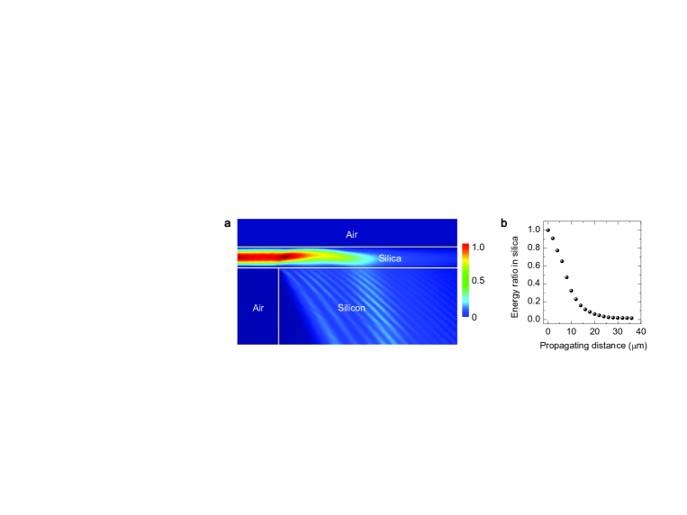
Figure 3: (a) Finite-element-method modeling the light propagating inside the $2$-$\mathrm{\mu}$m-thick silica waveguide bonding with a thick silicon layer. (b) Remaining energy ratio in silica vs. the propagating distance.

V Fiber taper and free-space coupling

In Fig. 4(a) we provide an independent cross-check that many high-$Q$ modes ($Q>10^{5}$) do exist in the deformed microcavity, by exciting them directly through a tapered fiber. Here the silicon pillar attached to the microtoroid has largest size, so that dynamical tunneling is inhibited and no WGM can be excited with the free-space coupling [Fig. 4(c)]. By reducing the size of the silicon pillar, as shown in Fig. 3 in the main text, high-$Q$ modes can be excited indirectly by a free-space beam.

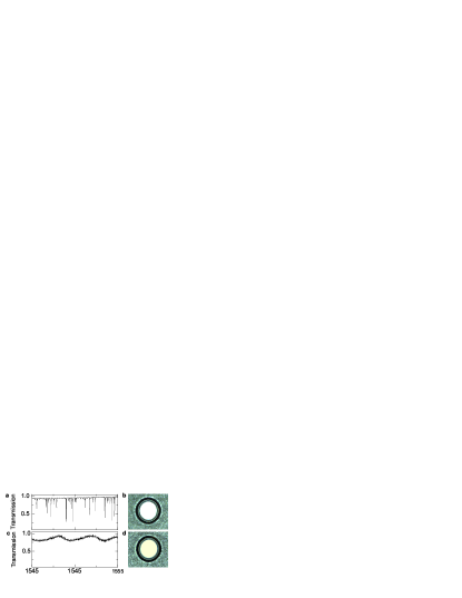
Figure 4: Normalized transmission and top-view images of the cavity coupled by fiber taper [(a) and (b)] and free-space laser beam [(c) and (d)]. The absorber-to-cavity ratio $r\simeq 0.83$.

VI counting modes in transmission spectra

From the transmission spectra collected by the photon receiver, we single out the modes that have relatively high $Q$ factors. In particular, we count those with $Q>10^{5}$. There are TE modes and TM modes, which have orthogonal polarization in the microcavity. A polarization controller is used to excite modes with one polarization, adjust the polarization to alternatively achieve the highest efficiencies for one kind of modes and suppress the other one. We counted the number of modes in the transmission spectra with both kind of polarizations and add them together to obtain the total number of high$-Q$ regular modes. The so called TE modes and TM modes are not perfectly orthogonal in the real microcavity, so that some modes may be counted twice, which is the source of the uncertainty in our data.

VII Ehrenfest time and Lyapunov exponent

We first give a brief explanation of how the semiclassical correction Eq. (4) of the main text was obtained in reference [39]. Our first goal is to estimate the fraction of trajectories that escape within the so called Ehrenfest time $\tau_{Ehr}$, that is the time of quantum-to-classical correspondence. For an open system, $\tau_{Ehr}$ is the time it takes for a density as large as the size of the channels to be reduced to one Planck cell by the chaotic motion:

$$\frac{N}{M}e^{-\hat{\mu}t}=\frac{1}{M},$$ (2)

verified for $\tau_{Ehr}=\hat{\mu}^{-1}\log N$ (here $\hat{\mu}$ is proportional to the Lyapunov exponent of the closed system). Equation (2) can also be thought of as the mean time it takes for a wavepacket the size of a Planck cell to escape, driven by classical dynamics. We notice $\tau_{Ehr}$ is proportional to the logarithm of the number of channels, meaning a faster escape implies a longer quantum-to-classical correspondence. Classically, the probability for an initial area $A_{0}$ of the phase space to survive for a time $t$ is

$$P(t)\sim A_{0}e^{-t/\tau_{d}},$$ (3)

so that the probability for an area to survive in the phase space within Ehrenfest time is simply $P(\tau_{Ehr})\sim A_{0}e^{-\tau_{Ehr}/\tau_{d}}$. Now take $A_{0}=M$, total area of our phase space in units of $h$. From the definitions we gave of $\tau_{Ehr}=\hat{\mu}^{-1}\log N$, we can express the survival probability at Ehrenfest time in terms of the number of open channels and Lyapunov exponent, as $N^{-1/\hat{\mu}\tau_{d}}$, and therefore the number of surviving modes as

$$M(\tau_{Ehr})=MN^{-1/\hat{\mu}\tau_{d}},$$ (4)

as seen in Eq. (4) of the main text. In some sense, this is the ‘real’ Weyl law here, since its ‘fractality’ lies in the non-integral power.

The classical estimate of the prefactor $MN^{-1/\tau_{d}}$ involves Ehrenfest time, defined for open systems as

$$\tau_{Ehr}=\frac{1}{\mu}\log\frac{\tau_{H}}{\tau_{d}}.$$ (5)

Here $\mu$ is the Lyapunov exponent of the closed system, $\tau_{d}$ is the dwelling time that we are already familiar with, while $\tau_{H}$ is the Heisenberg time

$$\tau_{H}=\frac{h}{\Delta E},$$ (6)

with $\Delta E$ mean level spacing, that is average distance (or difference) bewteen consecutive energy levels. We know, on the other hand, that $E=h\nu$, and we may therefore express Heisenberg time in terms of the frequency spacing

$$\tau_{H}=\frac{1}{\Delta\nu},$$ (7)

and Ehrenfest time as

$$\tau_{Ehr}=\frac{1}{\mu}\log\frac{N}{\Delta\Upsilon}.$$ (8)

Here $N$ is the number of open channels as we know, whereas $\Delta\Upsilon=MT\Delta\nu$, that is the mean frequency spacing times the Poincaré time (to make it dimensionless), times the number of states $M$. In plain words, $\Delta\Upsilon$ is the frequency range of our modes in units of the Poincaré time. At this point we can still write

$$\tau_{Ehr}=\frac{1}{\hat{\mu}}\log N,$$ (9)

provided that

$$\hat{\mu}=\frac{\log N}{\log N-\log\Delta\Upsilon}\mu.$$ (10)

Thus we have determined the rescaling to the Lyapunov exponent, following the definition of the Ehrenfest time.

We may give the rescaling factor an estimate, based on our experimental setup. Taking for example $T=\frac{a}{2c}~{}\simeq 4\cdot 10^{-13}$s ($a$ is the diameter of the cavity, $c$ the speed of light in the silica), $\lambda=6.35\cdot 10^{-7}$m (visible light), the mean wavelength spacing (from the spectra) as $\Delta\lambda\sim 10^{-10}$m, we estimate $\Delta\nu=\frac{c\Delta\lambda}{\lambda^{2}}\sim 10^{11}$Hz. Moreover, the total number of states is estimated as $M\simeq Aa/\lambda\simeq 40$, with $A$ area of the phase space in exam, while the mean number of open channels is estimated by the same expression with a smaller area, indicating the open strip of the phase space. Using the figures above, we get that

$$\hat{\mu}\simeq 1.3\mu.$$ (11)

This correction turns out to be within the uncertainties of the average finite-time Lyapunov exponent numerically computed for the open billiard, and therefore it has been neglected.

VIII $\chi^{2}$ test

The expression for the $\chi^{2}$ test used to assess the goodness of our fits is

$$\chi^{2}=\frac{1}{\nu}\sum\frac{(x_{\text{{ob}}}-x_{\text{{th}}})^{2}}{\sigma^{2}},$$ (12)

$x_{\text{{ob}}}$ being the observed datum, $x_{\text{{th}}}$ its theoretical expectation, $\sigma^{2}$ the experimental uncertainty, and $\nu$ the number of degrees of freedom. In general, $\chi^{2}\gg 1$ indicates a poor model fit, while $\chi^{2}>1$ indicates that the fit has not fully captured the data (or that the error variance has been underestimated). In principle, a value of $\chi^{2}=1$ indicates that the extent of the match between observations and estimates is in accord with the error variance. The limit of $\chi^{2}<1$ indicates that the model is over-fitting the data: either the model is improperly fitting noise, or the error variance has been overestimated.

IX More experimental and fitting results

In Fig. 5 we show more experimental and fitting results. Fig. 5(a)-(c) are in the infrared wavelength band and (d),(e) are in the visible wavelength band. All of them support our claim in the main text that the semiclassical correction (red solid curves) fits the experimental data better than the purely RMT-based estimate (blue dashed curves), especially at smaller deformation, where the two predictions differ the most.

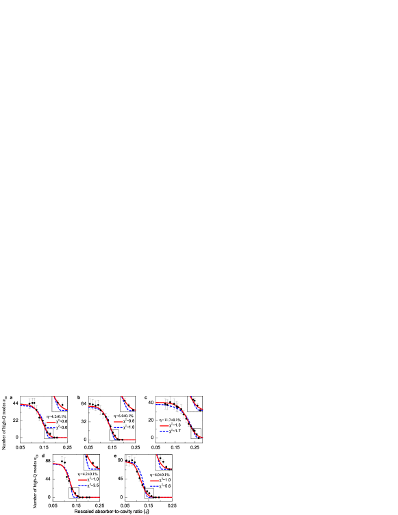
Figure 5: (color online) Number of high-$Q$ regular modes ($n_{\omega}$) observed in the transmission spectra of the microcavity (Dots), as a function of rescaled absorber-to-cavity ratio $\xi$. Blue dashed and red solid curves are respectively RMT- and semiclassical prediction best fits. Here $\sin\theta_{c}\simeq 0.69$ and $\sin\theta_{\mathrm{th}}=0.6$. Inset: the area where the two curves differ most.

X Table of parameters

We report the parameters used in our fittings in the following tables

Table 1: Quantities used in relation to the RMT-based expression (Eq.(6) of the main text). $\gamma$ is in unit of $T^{-1}$, with $T\simeq 4\cdot 10^{-13}$s Poincaré time.

$\Gamma$	$\gamma$	$\eta$	$\lambda(\mathrm{nm})$	$M$	$\tilde{\chi}^{2}$
5.2	0.15	4.2%	630	40	3.5
3.2	0.19	4.2%	1550	20	3.6
7.2	0.16	6.0%	630	40	5.6
3.6	0.18	6.0%	1550	20	1.8
4.7	0.31	11.7%	1550	25	1.7

Table 2: Quantities used in relation to the semiclassical prediction (Eq.(7) of the main text). Both $\gamma$ and $\mu$ are in units of $T^{-1}$, with $T\simeq 4\cdot 10^{-13}$s Poincaré time.

$\Gamma$	$\gamma$	$\eta$	$\lambda(\mathrm{nm})$	$M$	$\mu$	$\tilde{\chi}^{2}$
2.9	0.19	4.2%	630	40	0.13	1.0
2.0	0.23	4.2%	1550	20	0.13	0.8
5.0	0.20	6.0%	630	40	0.15	1.0
2.5	0.21	6.0%	1550	20	0.15	0.8
1.5	0.38	11.7%	1550	25	0.21	1.3

XI Phase space with a small deformation factor

The phase space reported in the main text [Fig. 1(b)] belongs to a microcavity with relatively large deformation factor, $\eta=11.7\%$. Here we report the classical phase space of the microcavity with the deformation factor $\eta=4.2\%$ (Fig. 6), together with the survival probability of a ray in the chaotic region, obtained by analogously to the result shown in Fig. 5 of the main text. One can see here as well an overall algebraic decay of the survival probability, and a short-time (transient) hyperbolic behavior.

Figure 6: (a) Poincaré surface of section of the microcavity with deformation factor $\eta=4.2\%$. Red solid line indicates the angle of total internal reflection. (b) (logarithmic scale) Points: average survival probability $P(t)$ of a ray in the microcavity vs. $t$ (in units of Poincaré time) at $\xi=0.1$, from $10^{6}$ randomly-started trajectories. Line: the ansatz $P(t)=\mathrm{exp}(-t/\tau_{d})$, $\tau_{d}=14$. Inset: the long-time simulation showing algebraic decay.

XII Decay rates of WGMs and coupling to chaotic modes

The approximations

$$\sum_{n}f_{n}\frac{V_{n}}{\gamma_{n}}\sim n_{\gamma}\frac{\bar{f}\bar{V}}{\bar{\gamma}},$$

$$\sum_{n}\frac{V_{n}^{2}}{\gamma_{n}}\sim n_{\gamma}\frac{\bar{V}^{2}}{\bar{\gamma}}.$$ (13)

leading to Eq. (3) in the main text for the probability of excitation of a WGM may be thought of as too rough. In particular, the second expression in (13) means that we are ignoring the fluctuations of both the coupling and the decay of the chaotic modes in consideration. In order to show that we are allowed to do so, we shall take a step back and rewrite the expression for the amplitude

$$a_{\omega}=\frac{E_{0}\sum_{n}f_{n}\frac{V_{n}}{\gamma_{n}}}{\left[\gamma_{\omega}+i(\omega-\omega_{0})\right]+\sum_{n}\frac{V_{n}^{2}}{\gamma_{n}}}.$$ (14)

Here we recognize the total decay rate of the WGM of frequency $\omega$ as

$$\gamma_{\omega}^{tot}=\gamma_{\omega}+\sum_{n}\frac{V_{n}^{2}}{\gamma_{n}}\simeq\gamma_{\omega}+n_{\omega}\frac{\bar{V}^{2}}{\bar{\gamma}},$$ (15)

where the first term indicates the intrinsic linewidth of the WGM, while the second represents the decay into the chaotic modes. That already suggests that the larger $n$ , the larger $\gamma_{tot}$. If we can really ignore the fluctuations $\gamma_{\omega}$ in $V$ and $\gamma$, we should be able to see that trend. The problem is that we do not count $n$ directly, and thus we need to express $\gamma_{tot}$ in terms of some measurable quantity. A good candidate would be then $n_{\omega}$, the number of excited WGMs. And that reminds us of another important approximation:

$$|a_{\omega}|^{2}=\epsilon^{2}\frac{n_{\gamma}^{2}}{\Gamma^{2}+n_{\gamma}^{2}}.$$ (16)

where $\kappa$ is unknown. The assumption is that the number of excited WGMs is simply proportional to the probability of excitation of one WGM, where, in reality, $\Gamma=\gamma_{\omega}\bar{\gamma}/\bar{V}^{2}$ should be a function of $\omega$, that is even the average coupling of each regular mode to the chaotic sea depends on where the mode is supported, in the phase space. It would appear from the literature on dynamical tunneling [e.g. A. Bäcker et al., Phys. Rev. Lett. 100, 104101 (2008)] that we are not allowed to ignore the dependence of $\Gamma$ on $\omega$ as we did, since the couplings $V$ stretch over several orders of magnitude, depending on the regular mode in question. Still, suppose for a moment we can go on making that approximation. Eq. (15) would become, in terms of $n_{\omega}$,

$$\gamma_{\omega}^{tot}=\gamma_{\omega}\left(1+\sqrt{\frac{n_{\omega}}{\kappa-n_{\omega}}}\right)$$ (17)

The advantage of this equation is that we have experimental data to fit it to. Figure 7 shows that Eq. (17) does qualitatively capture the behavior of the average linewidths of the WGMs, within some errors. The fitted value for $\gamma_{\omega}$ corresponds to an average intrinsic $Q$ factor of the order of $10^{5}$, which is realistic. Importantly, the overall enlargement of the average linewidths with the number of observed WGMs constitutes independent evidence for the approximations leading to Eq. (16) to be reasonable for our experiment.

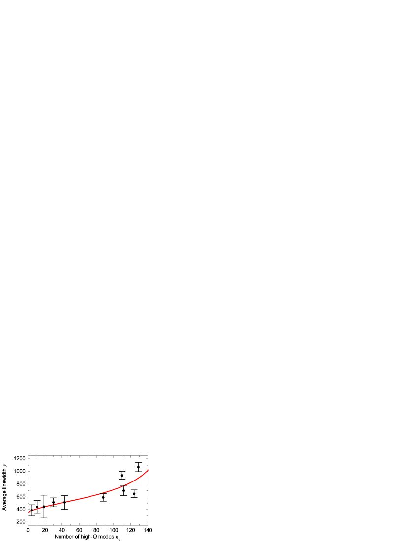
Figure 7: Points: average linewidth of the excited WGMs vs. their number. Each data point represents one experiment with a different size of the silicon pillar. As we know, the number of observed WGMs increases as the size of the pillar decreases. Line: Eq. (17), with $\gamma_{\omega}=326$, and $\kappa=171$.

References

- (1) C. Ellegaard, T. Guhr, K. Lindemann, J. Nygård, and M. Oxborrow, Symmetry Breaking and Spectral Statistics of Acoustic Resonances in Quartz Blocks, Phys. Rev. Lett. 77 , 4918 (1996).
- (2) G. E. Mitchell, A. Richter, and H. A. Weidenmüller, Random matrices and chaos in nuclear physics: Nuclear reactions, Rev. Mod. Phys. 82, 2845 (2010).
- (3) A. Frisch, M. Mark, K. Aikawa, F. Ferlaino, J. L. Bohn, C. Makrides, A. Petrov, and S. Kotochigova, Quantum chaos in ultracold collisions of gas-phase erbium atoms, Nature (London) 507, 475 (2014).
- (4) P. Carpena, P. Bernaola-Galvàn, P. Ch. Ivanov, and H. E. Stanley, Metalinsulator transition in chains with correlated disorder, Nature (London) 418, 955 (2002).
- (5) H. Cao and J. Wiersig, Dielectric microcavities: Model systems for wave chaos and non-Hermitian physics, Rev. Mod. Phys. 87, 61 (2015).
- (6) K. Pance, W. Lu, and S. Sridhar, Quantum Fingerprints of Classical Ruelle-Pollicott Resonances, Phys. Rev. Lett. 85, 2737 (2000).
- (7) A. Wirzba , Quantum mechanics and semiclassics of hyperbolic n-disk scattering systems, Phys. Rep. 309, 1-116 (1999).
- (8) J. A. Folk, S. R. Patel, S. F. Godijn, A. G. Huibers, S. M. Cronenwett, C. M. Marcus, K. Kampman, and A. C. Gossard, Statistics and Parametric Correlations of Coulomb Blockade Peak Fluctuations in Quantum Dots, Phys. Rev. Lett. 76, 1699 (1996).
- (9) M. V. Berry and M. Robnik, Semiclassical level spacings when regular and chaotic orbits coexist, J. Phys. A 17, 2413 (1984).
- (10) P. Gaspard and S. A. Rice, Semiclassical quantization of the scattering from a classically chaotic repellor, J. Chem. Phys. 90, 2242-2254 (1989).
- (11) P. So, S. M. Anlage, E. Ott, and R. N. Oerter, Wave Chaos Experiments With and Without Time Reversal Symmetry: GUE and GOE Statistics, Phys. Rev. Lett. 74, 2662 (1995)
- (12) E. N. Pozzo, D. Domínguez, and M. J. Sánchez, Quantum chaos in the mesoscopic device for the Josephson flux qubit, Phys. Rev. B 77, 024518 (2008).
- (13) O. A. Starykh, P. R. J. Jacquod, E. E. Narimanov, and A. D. Stone, Signature of dynamical localization in the resonance width distribution of wave-chaotic dielectric cavities, Phys. Rev. E 62, 2078 (2000).
- (14) G. Hackenbroich, Statistical theory of multimode random lasers, J. Phys. A 38, 10537 (2005).
- (15) H. Schomerus, J. Wiersig, and J. Main, Lifetime statistics in chaotic dielectric microresonators, Phys. Rev. A 79, 053806 (2009).
- (16) C. Liu, A. D. Falco, D. Molinari, Y. Khan, B. S. Ooi, T. F. Krauss, and A. Fratalocchi, Enhanced energy storage in chaotic optical resonators, Nat Photonics. 7, 473-478 (2013).
- (17) J. Yang, S.-B. Lee, S. Moon, S.-Y. Lee, S. W. Kim, T. T. A. Dao, J.-H. Lee, and K. An, Pump-Induced Dynamical Tunneling in a Deformed Microcavity Laser, Phys. Rev. Lett. 104, 243601 (2010).
- (18) Y.-F. Xiao, X.-F. Jiang, Q.-F. Yang, L. Wang, K. Shi, Y. Li, and Q. Gong, Tunneling-induced transparency in a chaotic microcavity, Laser Photonics Rev. 7, L51 (2013).
- (19) W. T. Lu, S. Sridhar, and M. Zworski, Fractal Weyl Laws for Chaotic Open Systems, Phys. Rev. Lett. 91, 154101 (2003).
- (20) M. J. Körber, M. Michler, A. Bäcker, and R. Ketzmerick, Hierarchical FractalWeyl Laws for Chaotic Resonance States in Open Mixed Systems, Phys. Rev. Lett. 111, 114102 (2013).
- (21) A. Ishii, A. Akaishi, A. Shudo, and H. Schomerus, Weyl law for open systems with sharply divided mixed phase space, Phys. Rev. E 85, 046203 (2012).
- (22) A. Potzuweit, T. Weich, S. Barkhofen, U. Kuhl, H.-J. Stöckmann, and M. Zworski, Weyl asymptotics: From closed to open systems, Phys. Rev. E 86, 066205 (2012).
- (23) S. Barkhofen, T. Weich, A. Potzuweit, H.-J. Stöckmann, U. Kuhl, and M. Zworski, Experimental observation of the spectral gap in microwave n-disk systems, Phys. Rev. Lett. 110, 164102 (2013).
- (24) S. Nonnenmacher and E. Schenck, Resonance distribution in open quantum chaotic systems, Phys. Rev. E 78, 045202 (2008).
- (25) M. Schönwetter and E. G. Altmann, Quantum signatures of classical multifractal measures, Phys. Rev. E 91, 012919 (2015).
- (26) J. Wiersig and J. Main, Fractal Weyl law for chaotic microcavities: Fresnel’s laws imply multifractal scattering, Phys. Rev. E 77, 036205 (2008).
- (27) M. J. Davis and E. J. Heller, Quantum dynamical tunneling in bound states, J. Chem. Phys 75, 246-254 (1981).
- (28) O. Bohigas, S. Tomsovic, and D. Ullmo, Manifestations of classical phase space structures in quantum mechanics, Phys. Rep. 223,43-133 (1993).
- (29) A. Bäcker, R. Ketzmerick, S. Löck, and L. Schilling, Regular-to-chaotic tunneling rates using a fictitious integrable system, Phys. Rev. Lett. 100, 104101(2008).
- (30) U. Fano, Effects of configuration interaction on intensities and phase shifts, Phys. Rev 124, 1866 (1961).
- (31) K. An and J. Yang, Mode-mode coupling theory of resonant pumping via dynamical tunneling processes in a deformed microcavity, in Trends in Nano- and Micro-Cavities, Bentham Science, Sharjah, U. A. E.(2011), pp.40-61.
- (32) See Supplemental Information for details.
- (33) H. Schomerus and J. Tworzydlo, Quantum-to-classical crossover of quasibound states in open quantum systems, Phys. Rev. Lett 93, 154102 (2004).
- (34) H. Schomerus and P. Jacquod, Quantum-to-classical correspondence in open chaotic systems, J. Phys. A 38, 10663 (2005).
- (35) K. Zyczkowski and H. J. Sommers, Truncations of random unitary matrices, J. Phys. A 33, 2045 (2000).
- (36) In what follows we neglect the dependence of on by taking the average value, which is determined by the ratio of the mean radius of the absorber to the cavity’s.
- (37) Since we do not have an estimate for the parameter , all the data sets are fitted up to a multiplicative constant.
- (38) J. R. Taylor, An introduction to error analysis, University Science Books, Sauselito, CA,(1997).
- (39) is computed over a short enough time for the dynamics to be still hyperbolic.
- (40) J. Meiss, Symplectic maps, variational principles, and transport, Rev. Mod. Phys. 64, 79 (1992).
- (41) M. Michler, A. Bäcker, R. Ketzmerick, H.-J. Stöckmann, and S. Tomsovic, Universal quantum localizing transition of a partial barrier in a chaotic sea, Phys. Rev. Lett. 109, 234101, (2012).
- (42) Y. C. Lai, and T. Tél, Transient Chaos, (Springer, New York, 2010).