Measuring higher-dimensional Entanglement

Abstract

We study local-realistic inequalities, Bell-type inequalities, for bipartite pure states of finite dimensional quantum systems – qudits. There are a number of proposed Bell-type inequalities for such systems. Our interest is in relating the value of Bell-type inequality function with a measure of entanglement. Interestingly, we find that one of these inequalities, the Son-Lee-Kim inequality, can be used to measure entanglement of a pure bipartite qudit state and a class of mixed two-qudit states. Unlike the majority of earlier schemes in this direction, where number of observables needed to characterize the entanglement increases with the dimension of the subsystems, this method needs only four observables. We also discuss the experimental feasibility of this scheme. It turns out that current experimental set ups can be used to measure the entanglement using our scheme.

I Introduction

In a much celebrated paper, J. S. Bell established that any realistic interpretation of quantum theory is bound to be nonlocal bell . Bell established this by means of an inequality which is violated by the singlet state of a pair of qubits. Later, it was shown that some other states also violate this inequality and thus forbid local-realistic description for them. All these led to a very natural question – whether this contradiction between quantum theory and local-realism is typical or it is restricted to some very special cases. Answer to this question came in 1991 when Nicolas Gisin gisin showed that any pure entangled state of a bipartite system violates a version of Bell’s inequality, Clauser-Horne-Shimony-Holt (CHSH) inequality chsh . Thus all pure bipartite states are nonlocal. The maximum quantum violation of this inequality is $2\sqrt{2}$. It is known as the Tsirelson’s bound tsirelson , which a two-qubit maximally entangled state attains for a particular measurement setting. This leads to another interesting question— is there any relation between violation of Bell’s inequality and amount of entanglement? In the case of two-qubit entangled states, it can be shown that there exist measurement settings for which value of the Bell-CHSH operator increases with the entanglement of the state. Is this also the case for two-qudit ($d>2$) entangled state? We answer this question also in affirmative.

Entanglement in higher dimensional systems is important from both fundamental and practical point of view. Higher dimensional entanglement provides important advantages in quantum communication than the conventional qubit entanglement. It provides more security against eavesdropping in cryptography durt , it can be used to increase the channel-capacity via superdense-coding chuang and is more robust against environmental noise pironio than the conventional two-qubit entanglement. However, for practical applications of these protocols, experimental preparation, detection and quantification of higher dimensional entangled state is of crucial importance. The violation of Bell-type inequalities can detect the presence of entanglement in such systems. Therefore, Bell-type inequalities in higher dimensional system have generated much interest in recent years peres ; cglmp ; slk ; korean ; dada ; hplo ; jphysA ; cdh . One of the approaches to obtain Bell-type inequality in higher dimension employs a projection of multilevel down to dichotomic one gisin ; peres . But sometimes it is also important to know whether it enables to probe genuine high-dimensionality or not cglmp ; slk ; cerf . In 2002, Collins, Gisin, Linden, Massar, and Popescu introduced cglmp an inequality (henceforth will be referred to as CGLMP inequality) which is known to be the only tight inequality massanes for higher dimensional systems. But, this inequality is not maximally violated for a maximally entangled state of such systems acin . Interestingly, in 2006, Son, Lee and Kim introduced another set of Bell-type inequalities for qudit systems (hereafter, the SLK inequality) slk which is maximally violated for a maximally entangled state of two-qudit. We show that for a particular measurement setting, the Bell-SLK function (defined below) is zero for product states. Thus, a nonzero value of this function immediately suggests that the measured state is entangled. Interestingly, for this setting, the value of the Bell-SLK function increases with the concurrence conc1 ; conc2 of the pure bipartite entangled states. Thus, the SLK test can serve as a measure of entanglement for pure bipartite states. The situation about mixed bipartite states of qudits is complicated. One needs a reliable entanglement measure for a general mixed state of qudits. Even for general bipartite qubit mixed states, the relation between entanglement and the value of CHSH function is not known. However, we find a relation between the entanglement of a class of mixed states, isotropic states, and the value of the Bell-SLK function for the state. We further explore the relationship between the entanglement, as measured using negativity, and the value of the Bell-SLK function for a maximally entangled state passed through noisy channels.

The widely adopted method for measuring entanglement of a state is the quantum state tomographic reconstruction tomography . In this method, a complete set of observables is measured on the system to reconstruct its state and thus to calculate the entanglement. Though, successfully implemented for lower-dimensional systems lowdimtomo1 , this method is not suitable for systems of higher dimension. This is because the number of observables to be measured increases dramatically with the dimension of the system highdimtomo1 . However, there are suggestions to characterize the state with less number of observables, but most of these methods are for two-qubit systems lowdimtomo2 . For higher dimensional systems, the alternative suggestions, though reduces the number of observables (in comparison to the traditional tomography), but the number is still high and increases with the dimension of the subsystems highdimtomo2 . In case of bipartite systems, the number of measurements needed is of the order of $d^{4}$ ($d$ is dimension of each subsystem) standatom . Moreover, the implementation of these observables in an experiment is also an issue to be taken proper considerationobexpfeasible . The measurement of the Bell-SLK function can be a method to measure entanglement of a pure bipartite state. Unlike the earlier schemes where number of observables needed depends on dimension of subsystems, this scheme needs measurement of only four observables to calculate the entanglement of any pure bipartite state. Moreover, this new scheme can be implemented in laboratories with the existing technology.

The paper is organized as follows. In Section II, we, discuss the SLK test and obtain a relation between the Bell-SLK function and the concurrence. We extend the study to mixed states in Section III. The way to measure the Bell-SLK function and hence the concurrence in laboratories is briefly discussed in Section IV. We conclude in Section V.

II The SLK inequality and concurrence

In the SLK test, two far separated observers Alice and Bob, can independently choose one of the two observables denoted by $A_{1}$, $A_{2}$ for Alice and $B_{1}$, $B_{2}$ for Bob. Measurement outcomes of the observables are elements of the set, $V=\{1,\omega,\cdots,\omega^{d-1}\}$, where $\omega=\exp{(2\pi i/d)}$. In a variant of SLK inequality korean , the Bell-SLK function, $I_{SLK}$, is given by

$$I_{SLK} = \frac{1}{\sqrt{2}}\sum\limits_{n=1}^{d-1}\big{(}\omega^{-n/4}C_{1,1}^{n}+\omega^{-3n/4}C_{2,1}^{n}$$ (1)

$$+\omega^{n/4}C_{1,2}^{n}+\omega^{-n/4}C_{2,2}^{n}\big{)}+c.c.,$$

$\omega=exp(2\pi i/d)$, c.c. is for complex conjugate, $C_{a,b}^{n}=\langle A_{a}^{n}B_{b}^{n}\rangle$. The assumption of local-realism implies $I_{SLK}\leq I_{SLK}^{\mbox{max}}\mbox{(LR)}$, where $I_{SLK}^{\mbox{max}}\mbox{(LR)}=\frac{1}{\sqrt{2}}\Big{(}3\cot\frac{\pi}{4d}-\cot\frac{3\pi}{4d}\Big{)}-2\sqrt{2}$ korean . By using Fourier transformation, we write Bell-SLK function in joint probability space as lcl ; korean

$$I_{SLK} = \sum\limits_{\alpha=0}^{d-1}f(\alpha)[P(A_{1}=B_{1}+\alpha)$$ (2)

$$+P(B_{1}=A_{2}+\alpha+1)+P(A_{2}=B_{2}+\alpha)$$

$$+P(B_{2}=A_{1}+\alpha)],$$

where sums inside the probabilities are modulo $d$ sums, and

$$f(\alpha)=\frac{1}{\sqrt{2}}\Big{(}\cot[\frac{\pi}{d}(\alpha+\frac{1}{4})]-1\Big{)}.$$ (3)

We now calculate the value of the Bell-SLK function for an arbitrary pure two-qudit state $|\psi\rangle=\sum_{i}c_{i}|ii\rangle$ and for the measurement settings originally given in dagomir . The nondegenerate eigenvectors of the operators $\hat{A_{a}}$, $a=1,2,$ and $\hat{B_{b}}$, $b=1,2,$ are respectively

$$|k\rangle_{A,a}=\frac{1}{\sqrt{d}}\sum\limits_{j=0}^{d-1}\omega^{(k+\delta_{a})j}|j\rangle,$$

$$|l\rangle_{B,b}=\frac{1}{\sqrt{d}}\sum\limits_{j=0}^{d-1}\omega^{(-l+\epsilon_{b})j}|j\rangle,$$ (4)

where $\delta_{1}=0,\delta_{2}=1/2,\epsilon_{1}=1/4$ and $\epsilon_{2}=-1/4.$ The joint probabilities in (2) can be calculated as

$$P(A_{1}=B_{1}+\alpha)=\frac{1}{d}\sum\limits_{p,q=0}^{d-1}c_{p}c_{q}\omega^{(\alpha+1/4)(p-q)},$$

$$P(B_{1}=A_{2}+\alpha+1)=\frac{1}{d}\sum\limits_{p,q=0}^{d-1}c_{p}c_{q}\omega^{-(\alpha+1/4)(p-q)},$$

$$P(A_{2}=B_{2}+\alpha)=\frac{1}{d}\sum\limits_{p,q=0}^{d-1}c_{p}c_{q}\omega^{(\alpha+1/4)(p-q)},$$

$$P(B_{2}=A_{1}+\alpha)=\frac{1}{d}\sum\limits_{p,q=0}^{d-1}c_{p}c_{q}\omega^{-(\alpha+1/4)(p-q)}.$$ (5)

Putting these probabilities in (2), we get

$$I_{SLK}=\frac{4}{d}\sum\limits_{\alpha=0}^{d-1}f(\alpha)\sum\limits_{p,q=0}^{d-1}c_{p}c_{q}\omega^{(\alpha+1/4)(p-q)}.$$ (6)

From the identity $\sum\limits_{k=0}^{d-1}(-1)^{k}\cot(\frac{2k+1}{4d})\pi=d$ Hassan , we can obtain another identity $\sum\limits_{k=0}^{d-1}\cot(\frac{4k+1}{4d})\pi=d$. Therefore, we get $\sum\limits_{\alpha=0}^{d-1}f(\alpha)=0$. We can then rewrite (6) as

$$I_{SLK} =\frac{4}{d}\sum\limits_{\alpha=0}^{d-1}f(\alpha)\sum_{\begin{subarray}{c}p\neq q\\ p>q\end{subarray}}2c_{p}c_{q}\cos\Big{(}\frac{2\pi}{d}(\alpha+\frac{1}{4})(p-q)\Big{)}$$ (7)

$$=\frac{4}{d}\sum\limits_{\alpha=0}^{d-1}\frac{1}{\sqrt{2}}\Big{(}\cot[\frac{\pi}{d}(\alpha+\frac{1}{4})]-1\Big{)}$$

$$\quad\quad\sum_{\begin{subarray}{c}p\neq q\\ p>q\end{subarray}}2c_{p}c_{q}\cos\Big{(}\frac{2\pi}{d}(\alpha+\frac{1}{4})(p-q)\Big{)}.$$

To evaluate it further, we now need to find following two sums

$$\sum\limits_{\alpha=0}^{d-1}\cos\Big{(}\frac{2\pi m}{d}(\alpha+\frac{1}{4})\Big{)},$$ (8)

and

$$\sum\limits_{\alpha=0}^{d-1}\cos\Big{(}\frac{2\pi m}{d}(\alpha+\frac{1}{4})\Big{)}\cot\Big{(}\frac{\pi}{d}(\alpha+\frac{1}{4})\Big{)},$$ (9)

where we have replaced $p-q$ by $m$ (an integer).

Using trigonometrical identity in Gradshteyn , we obtain

$$\sum\limits_{\alpha=0}^{d-1}\cos\Big{(}\frac{2\pi m}{d}(\alpha+\frac{1}{4})\Big{)}$$

$$=\cos\Big{(}\frac{\pi m}{2d}+\frac{(d-1)\pi m}{d}\Big{)}\sin\pi m\operatorname{cosec}\frac{\pi m}{d}$$

$$=0,$$ (10)

i.e, the first sum (8) is equal to zero.

To calculate the sum (9), we will need two sums that are not available in well known mathematics handbooks. Motivated by this, we have recently obtained a number of trigonometric functions sums cpsums . Here we need corollaries of the theorems in cpsums . So we only indicate how to obtain one sum. Other is obtained in the similar manner.

Proposition: With $a$ and $k$ being positive integer such that $a<k$, and $0<b<1$,

$$\sum\limits_{j=0}^{k-1}\cos{\frac{2\pi aj}{k}}\cot{(\frac{\pi j}{k}+\pi b)}$$

$$=k\cos{[b(2a-k)\pi]}\operatorname{cosec}{(bk\pi)},$$ (11)

Proof: To obtain the sum, we will use the method of residues. We take the complex function as Berndt

$$g_{1}(z)=\frac{e^{2\pi iaz}\cot{(\pi z+\pi b)}}{e^{2\pi ikz}-1}-\frac{e^{-2\pi iaz}\cot{(\pi z+\pi b)}}{e^{-2\pi ikz}-1}.$$ (12)

Let us now consider the integral $\frac{1}{2\pi i}\int_{C}g_{1}(z)dz$, where $C$ is a contour which is positively oriented indented rectangle with vertices at $\pm iR$ and $1\pm iR$, with $R>\epsilon$, and with semicircular indentations of radius $\epsilon<b$ to the left of both $0$ and $1$. Since the period of $g_{1}(z)$ is $1$, the integrals along the intended vertical sides of $C$ cancel. Here we have taken $a$ such that $0<a<k$. $g_{1}(z)$ tends to $0$ uniformly for $0\leqslant x\leqslant 1$ as $\lvert y\rvert\ \rightarrow\infty$. Hence, $\frac{1}{2\pi i}\int_{C}g_{1}(z)dz=0$. We, next, calculate the residue at different poles of $g_{1}(z)$. $g_{1}$ has simple poles at $z=0$ and $z=j/k,1\leqslant j\leqslant k-1$. The corresponding residues can be calculated as

$$\mbox{Res}(g_{1},0)=\frac{1}{\pi ik}\cot(\pi b),$$

$$\mbox{Res}(g_{1},j/k)=\sum\limits_{j=1}^{k-1}\frac{1}{\pi ik}\cos{\frac{2\pi aj}{k}}\cot{(\frac{\pi j}{k}+\pi b)}.$$ (13)

There is another pole inside the contour – simple pole at $z=-b+1$. The residue at this point is

$$\mbox{Res}(g_{1},-b+1)=\frac{i}{\pi}\cos{[b(2a-k)\pi]}\operatorname{cosec}{(bk\pi)}.$$ (14)

As the integral is zero, the sum of the residues must be zero. We, thus, get

$$\sum\limits_{j=0}^{k-1}\cos{\frac{2\pi aj}{k}}\cot{(\frac{\pi j}{k}+\pi b)}$$

$$=k\cos{[b(2a-k)\pi]}\operatorname{cosec}{(bk\pi)}.$$ (15)

This completes the proof footnote .

Similarly, we can obtain, with $a$ and $k$ being positive integer such that $a<k$, and $0<b<1$.

$$\sum\limits_{j=0}^{k-1}\sin{\frac{2\pi aj}{k}}\cot{(\frac{\pi j}{k}+\pi b)}$$

$$=-k\sin{[b(2a-k)\pi]}\operatorname{cosec}{(bk\pi)}.$$ (16)

Using above two results and sum and difference formula for cosines, we find.

$$\sum\limits_{\alpha=0}^{d-1}\cos\Big{(}\frac{2\pi m}{d}(\alpha+\frac{1}{4})\Big{)}\cot\Big{(}\frac{\pi}{d}(\alpha+\frac{1}{4})\Big{)}=d.$$ (17)

This sum is remarkably simple. We note that the value of this sum is independent of $m$. This is crucial in relating the value of the Bell-SLK function and entanglement.

Eqs. (3), (7), (10) and (17) together imply

$$I_{SLK}=4\sqrt{2}\sum_{\begin{subarray}{c}p\neq q\\ p>q\end{subarray}}c_{p}c_{q}.$$ (18)

This sum is proportional to the concurrence of the state. The concurrence, $\mathbb{C}$, for a two-qudit pure state is defined as conc1

$$\mathbb{C}=\sum_{\begin{subarray}{c}p\neq q\\ p>q\end{subarray}}c_{p}c_{q}\frac{2}{d-1}.$$ (19)

This is a generalization of the concurrence for a system of two qubits conc2 . Using this, we finally get

$$I_{SLK}=2\sqrt{2}(d-1)\mathbb{C}.$$ (20)

Thus, we obtain an interesting relation between concurrence and the value of the Bell-SLK function for a particular measurement setting. Value of this function is zero for product states whereas it increases linearly with the concurrence for pure entangled states bellfootnote . This gives a way to measure the entanglement of a pure entangled state. The entanglement can be calculated by measuring the Bell-SLK function for the state for the above, given in (4), measurement setting.

III Case of Mixed States

III.1 Isotropic States

As discussed earlier, the case of mixed states even for bipartite qubit systems is far from simple. In the case of mixed bipartite qudit states, one needs a proper measure of entanglement. For bipartite mixed states, the concurrence $\mathbb{C}(\rho)$ is calculated by the ‘convex-roof extension’ of the pure-state concurrence, i.e., by minimizing the average value of the concurrence (mentioned in Eq. (19)) over all ensemble decompositions of the mixed state $\rho$:

$$\mathbb{C}(\rho)=\inf\limits_{\{p_{i},|\psi_{i}\rangle\}}\Bigg{\{}\sum_{i}p_{i}\mathbb{C}(|\psi_{i}\rangle)\Bigg{|}\sum_{i}p_{i}|\psi_{i}\rangle\langle\psi_{i}|=\rho\Bigg{\}}.$$

Interestingly, in rungta_caves , this concurrence has been shown to be an entanglement monotone. However, due to extremization involved in the calculation, the concurrence in the closed form has been obtained only for a special class of mixed state, namely, for the isotropic states. For a two-qudit system, isotropic states are convex mixtures of the maximally entangled state,

$$|\Psi^{+}\rangle=\frac{1}{\sqrt{d}}\sum\limits_{j=0}^{d-1}|jj\rangle,$$ (21)

with a maximally mixed state $I=I\otimes I/d^{2}$. These states can be written as

$$\rho_{F}=\frac{1-F}{d^{2}-1}\big{(}I-|\Psi^{+}\rangle\langle\Psi^{+}|\big{)}+F|\Psi^{+}\rangle\langle\Psi^{+}|,$$ (22)

where $F$ is the fidelity of $\rho_{F}$ and $|\Psi^{+}\rangle$ satisfying $0\leqslant F\leqslant 1$. These states are separable for $F\leqslant 1/d$ rungta_horodecki .

In the following, we calculate the Bell-SLK function for these states. The Bell-SLK function $I_{SLK}$ (given in Eq. (2)) consists of four probabilities. Here, we calculate one of the probabilities, $P(A_{1}=B_{1}+\alpha)$, other probabilities can be calculated similarly.

$$P(A_{1}=B_{1}+\alpha)$$

$$=\mbox{Tr}\big{[}\hat{P}(A_{1}=B_{1}+\alpha)\rho_{F}\big{]}$$

$$=\frac{1-F}{d^{2}-1}\mbox{Tr}\big{[}\hat{P}(A_{1}=B_{1}+\alpha)I\big{]}+$$

$$\frac{d^{2}F-1}{d^{2}-1}\mbox{Tr}\big{[}\hat{P}(A_{1}=B_{1}+\alpha)|\Psi^{+}\rangle\langle\Psi^{+}|\big{]};$$ (23)

where $\hat{P}(A_{1}=B_{1}+\alpha)$ stands for appropriate projector. The first part of the above sum can be calculated as

$$\mbox{Tr}\big{[}\hat{P}(A_{1}=B_{1}+\alpha)I\big{]}$$

$$=\frac{1}{d^{2}}\sum_{i,j,p,q,l,m,n}\omega^{(l+\alpha)(i-j)}\omega^{(-l+1/4)(p-q)}$$

$$\langle m|i\rangle\langle j|m\rangle\langle n|p\rangle\langle q|n\rangle$$

$$=d$$ (24)

whereas the second part as

$$\mbox{Tr}\big{[}\hat{P}(A_{1}=B_{1}+\alpha)|\Psi^{+}\rangle\langle\Psi^{+}|\big{]}$$

$$=\langle\Psi^{+}|\hat{P}(A_{1}=B_{1}+\alpha)|\Psi^{+}\rangle$$

$$=\frac{1}{d^{3}}\sum_{i,j,l,r,s,p,q}\omega^{(l+\alpha)(r-s)}\omega^{(-l+1/4)(p-q)}$$

$$\langle i|r\rangle\langle i|p\rangle\langle s|j\rangle\langle q|j\rangle$$

$$=\frac{1}{d^{2}}\sum_{i,j}\omega^{(\alpha+1/4)(i-j)}.$$ (25)

The other three joint probabilities when calculated, come out to be equal to the probability calculated above. The Bell-SLK function, $I_{SLK}$ can now be obtained, by putting for these probabilities in Eq. (2), as:

$$I_{SLK} = \bigg{(}\frac{1-F}{d^{2}-1}\bigg{)}4d\sum\limits_{\alpha=0}^{d-1}f(\alpha)+$$ (26)

$$\bigg{(}\frac{d^{2}F-1}{d^{2}-1}\bigg{)}\frac{4}{d^{2}}\sum\limits_{i,j,\alpha=0}^{d-1}f(\alpha)\omega^{(\alpha+1/4)(i-j)}.$$

Using the fact that $\sum\limits_{\alpha=0}^{d-1}f(\alpha)=0$ (This has been shown in Section II.), the Bell-SLK function reads

$$I_{SLK}=\bigg{(}\frac{d^{2}F-1}{d^{2}-1}\bigg{)}\frac{4}{d^{2}}\sum\limits_{i,j,\alpha=0}^{d-1}f(\alpha)\omega^{(\alpha+1/4)(i-j)}.$$ (27)

Proceeding now in a manner similar as in section (II), we get the Bell-SLK function as

$$I_{SLK}=\frac{2\sqrt{2}}{d+1}(d^{2}F-1).$$ (28)

The concurrence $\mathbb{C}(\rho_{F})$ for isotropic states (with some normalization) has been calculated in rungta_caves as

$$\mathbb{C}(\rho_{F})=\begin{cases}0,&F\leqslant 1/d,\\ \frac{dF-1}{d-1},&1/d\leqslant F\leqslant 1.\end{cases}$$ (29)

Using Eq.(29) in Eq. (28), we can be rewrite the later equation to read as

$$I_{SLK}=\begin{cases}\frac{2\sqrt{2}}{d+1}(d^{2}F-1),&F\leqslant 1/d,\\ \frac{2\sqrt{2}}{d+1}\big{(}(d-1)(d\mathbb{C}(\rho_{F})+1)\big{)},&1/d\leqslant F\leqslant 1.\end{cases}$$ (30)

Thus, we get an interesting relation between the Bell-SLK function and the concurrence for isotropic states. It can easily be checked that for $F\leqslant 1/d$, i.e. for the separable isotropic states, the value of the Bell-SLK function is upper bounded by the $\frac{2\sqrt{2}}{d+1}(d-1)$. A value larger than this bound, immediately suggests that the isotropic states undergoing the said Bell-SLK measurements are entangled and their entanglement increases with the value of the Bell-SLK function.

III.2 Maximally Entangled state through a noisy channel

In this section, we will consider another class of mixed states that are obtained when particles in a maximally entangled state pass through noisy channels. This is often a real laboratory situation. As we have already mentioned there is no closed from of concurrence for a general mixed state of two qudits; so here we use another measure of entanglement, called negativity vidal . The negativity of a state $\rho$ is defined as

$$\mathcal{N}(\rho)=\frac{||\rho^{T_{B}}||_{1}-1}{d-1},$$ (31)

where $||\cdot||_{1}$ represents the trace norm and $\rho^{T_{B}}$ is the partial transpose of the state $\rho$ with respect to the subsystem $B$. For a pure state $|\psi\rangle=\sum_{i}c_{i}|ii\rangle$ the negativity can be written as soojoon

$$\mathcal{N}\big{(}|\psi\rangle\langle\psi|\big{)}=\sum_{\begin{subarray}{c}p\neq q\\ p>q\end{subarray}}c_{p}c_{q}\frac{2}{d-1},$$ (32)

where $c_{i}$ are the Schmidt coefficients. So it is same as concurrence for a pure state. Therefore, we can write (20) also as

$$I_{SLK}=2\sqrt{2}(d-1)\mathcal{N}.$$ (33)

Let’s say a party prepares a maximally entangled state and sends it to two distant parties by some noisy channels. The state will no longer be a pure state. Since we can compute negativity for a mixed state, we can explore the relationship between negativity and the value of the Bell-SLK function. We can also find how robust is the measurement of entanglement of a pure state using the Bell-SLK function. We will study this situation in $d=3$ taking two well known channels – the amplitude damping and the phase damping channels.

III.2.1 Amplitude damping

Let us consider a maximally entangled state $|\psi\rangle=\frac{1}{\sqrt{3}}(|00\rangle+|11\rangle+|22\rangle)$. Two qutrits are sent to distant parties through amplitude damping channels. For a qutrit, amplitude damping channel can be represented in terms of Kraus operators as ramzan

$K_{0}=\begin{pmatrix}1&0&0\\ 0&\sqrt{1-p}&0\\ 0&0&\sqrt{1-p}\end{pmatrix}$,

$K_{1}=\begin{pmatrix}0&\sqrt{p}&0\\ 0&0&0\\ 0&0&0\end{pmatrix}$, $K_{2}=\begin{pmatrix}0&0&\sqrt{p}\\ 0&0&0\\ 0&0&0\end{pmatrix}$,
where $p$ is the channel parameter. For simplicity we take same channel on both sides. We find that, without noise, the value of $I_{SLK}$ is $5.657$ and negativity is $\mathcal{N}=1$. At $90\%$ purity (purity varies with the channel parameter, $p$) $I_{SLK}=5.359$ and negativity is $\mathcal{N}=0.922$. So the value of negativity is about $8\%$ lower. However, it turns out that there is still a relationship between the value of the Bell-SLK function and entanglement for such states. From the value of the Bell-SLK function we can infer the entanglement of the state in terms of negativity. This is clear from Figure1 that looking at the $I_{SLK}$ curve, we can find state’s negativity at any purity.

Figure 1: Change in the Bell-SLK function and negativity with purity for a maximally entangled two-qutrit state passed through the amplitude damping channel.

III.2.2 Phase damping

Let us now consider the case when the two qutrits in a maximally entangled state pass through phase damping channels separately. The Kraus operators for the phase damping channel are ramzan

$K_{0}=\sqrt{1-p}\begin{pmatrix}1&0&0\\ 0&1&0\\ 0&0&1\end{pmatrix}$ and $K_{1}=\sqrt{p}\begin{pmatrix}1&0&0\\ 0&\omega&0\\ 0&0&\omega^{2}\end{pmatrix}$,
where $\omega=e^{\frac{2\pi i}{3}}$ and $p$ is the channel parameter. We do the same analysis as for the amplitude damping channel. At $90\%$ purity $I_{SLK}=5.209$ and $\mathcal{N}=0.922$. Both values decrease by about $8\%$, as compared to the starting pure state. However, as before, from Figure2, we notice an interesting relationship between entanglement and the value of the Bell-SLK function. If we measure the $I_{SLK}$ value for the state, we can easily determine the entanglement of the state in terms of negativity.

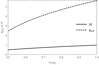
Figure 2: Change in the Bell-SLK function and negativity with purity for a maximally entangled two-qutrit state passed through the phase damping channel.

IV An Experimental scheme

Interestingly, this SLK test can be performed in laboratories with the present day’s technology dada ; hplo . One technique to encode a state of a qudit is to use the orbital angular momentum (OAM) states of photons zeilinger1 . Higher dimensional bipartite entanglement is generated through spontaneous parametric down conversion (SPDC) zeilinger2 ; dada . In dada , Dada et al. have employed the same measurement setting as in Eq. (II) to obtain the violation of CGLMP inequality for bipartite qudit systems with dimensions up to twelve. One can use the same experimental set up to measure the Bell-SLK function (instead of the CGLMP function as done in dada ) in order to find the amount of entanglement present in a pure bipartite state. In this case, four observables are to be measured. However, in this experimental set up, the measurement of each observable requires $(d-1)$ experimental settings. The number of settings varies linearly with respect to the dimension $d$. In principle, it might be possible to reduce the number of settings to measure an observable with $d$ outcomes. In hplo , Lo et al. employ a different experimental set up.They simulate qudits using multiple pairs of polarization-entangled photons. They also measure four observables with $(d-1)$ experimental settings for each observable and demonstrate the violation of CGLMP inequality up to $d=16$. Though violation of the CGLMP inequality can detect the presence of entanglement, but this violation cannot be used to measure the amount of entanglement present in the bipartite state, at least, for the employed setting. This is because, for these settings, CGLMP inequality is not maximally violated for a maximally entangled state of two qudits acin . It is also known acin that CGLMP inequality is violated maximally by a partially entangled state. Therefore, it is unlikely that CGLMP function measurement can help in measuring the amount of entanglement in a two-qudit state. As is known, the choice of measurement setting is important. There are measurement settings, for which even maximally entangled state may not violate an inequality. One of the key mathematical reason for the relation (20) to exist is that the sum (17) is independent of $m$. In the case of CGLMP inequality, the function $f(\alpha)$ is different, therefore a different sum occurs. That sum is not independent of $m$. Therefore, such a relation does not exist for the CGLMP inequality. However the measurement of the Bell-SLK function can help us in finding the amount of entanglement in a pure two-qudit state.

V Conclusion

In conclusion, we have studied Bell-type inequalities for bipartite qudit systems. There are many such local-realistic inequalities present in the literature. We have argued that one such inequality, namely the SLK inequality, can be useful in measuring the entanglement present in such systems. This also addresses an important question in entanglement theory: How to measure amount of entanglement for a bipartite state experimentally. The earlier methods for measuring entanglement requires number of observables to increase with dimension of the subsystems. In contrast, the scheme presented here requires only four observables to be measured to find the amount of entanglement present in a bipartite pure state. The scheme also works for a class of bipartite mixed qudit states – isotropic states. We have also considered the case of mixed states which are obtained after applying phase or amplitude damping channels on two qutrits which are in maximally entangled state. It appears that for such states one can also measure entanglement, as characterized by negativity. We have also discussed the experimental feasibility of our scheme. Current state-of-the-art allows experimental measurement of these observables (as in Eq. (II)) with $d-1$ settings to measure $d$ possible outcomes of each observable hplo . Improvements in the experimental set up may allow the measurement of each observable with fewer settings.

VI Acknowledgment

S.K.C. acknowledges support from the Council of Scientific and Industrial Research, Government of India (Scientists’ Pool Scheme).

References

- (1) J. S. Bell Physics 1 195 (1964); J. S. Bell Rev. Mod. Phys. 38 447 (1966).
- (2) N. Gisin Phys. Lett. A 154 201 (1991).
- (3) J. F. Clauser, M. A. Horne, A. Shimony, R. A. Holt, Phys. Rev. Lett. 23 880 (1969).
- (4) B. S. Tsirelson Lett. Math. Phys. 4 93 (1980).
- (5) H. Bechmann-Pasquinucci and A. Peres Phys. Rev. Lett. 85 3313 (2000); D. Bruss and C. Macchiavello Phys. Rev. Lett. 88 127901 (2002); T. Durt, N. J. Cerf, N. Gisin and M. Zukowski Phys. Rev. A 67 012311 (2003); T. Durt, D. Kaszlikowski, J. L. Chen and L. C. Kwek Phys. Rev. A 69 032313 (2004).
- (6) C. Wang, F.-G. Deng, Y.-S. Li, X.-S. Liu and G. L. Long Phys. Rev. A 71 044305 (2005).
- (7) M. L. Almeida, S. Pironio, J. Barrett, G. Toth, and A. Acin, Phys. Rev. Lett. 99 040403 (2007); L. Sheridan and V. Scarani Phys. Rev. A 82 030301 (2010).
- (8) N. Gisin and A. Peres Phys. Lett. A 162 15 (1992).
- (9) D. Collins, N. Gisin, N. Linden, S. Massar, and S. Popescu Phys. Rev. Lett. 88 040404 (2002).
- (10) W. Son, J. Lee and M. S. Kim Phys. Rev. Lett. 96 060406 (2006).
- (11) S.-W. Lee, J. Ryu, and J. Lee Journal of the Korean Physical Society, Vol. 48 No. 6, 1307 (2006).
- (12) A. C. Dada, J. Leach, G. S. Buller, M. J. Padgett and E. Andersson Nature Physics 7 677 (2011).
- (13) H.-P. Lo et al. Sci. Rep. 6, 22088 (2016).
- (14) C. Bernhard, B. Bessire, A. Montina, M. Pfaffhauser, A. Stefanov and S. Wolf J. Phys A: Math. Theor. 47 424013 (15pp) (2014).
- (15) J.-L. Chen, D.-L. Deng, and M.-G. Hu, Phys. Rev. A 77 060306(R) (2008).
- (16) N. J. Cerf, S. Massar and S. Pironio Phys. Rev. Lett. 89, 080402 (2002).
- (17) L. Masanes, Quantum Inf. Comput. Vol. 3, No. 4, 345 (2003).
- (18) A. Acin, T. Durt, N. Gisin and J. I. Latorre Phys. Rev. A 65 052325 (2002).
- (19) P. Rungta, V. Buzek, C. M. Caves, M. Hillery, and G. J. Milburn, Phys. Rev. A 64 042315 (2001).
- (20) W. K. Wootters, Phys. Rev. Lett. 80 2245 (1998).
- (21) D. F. V. James, P. G. Kwiat, W. J. Munro, and A. G. White Phys. Rev. A 64 052312 (2001); M. Cramer et al. Nat. Commun. 1 149 (2010); M. Mohammadi, A. M. Brańczyk, and D. F. V. James Phys. Rev. A 87 012117 (2013); T. Jullien et al. Nat. Lett. 514 603 (2014).
- (22) A. G. White, D. F. V. James, P. H. Eberhard, and P. G. Kwiat Phys. Rev. Lett 83 3103 (1999); J. M. G. Sancho and S. F. Huelga Phys. Rev. A 61 042303 (2000); W. Laskowski, D. Richart, C. Schwemmer, T. Paterek, and H. Weinfurter Phys. Rev. Lett 108 240501 (2012).
- (23) J. T. Barreiro et al. Nat. Phys. 9 559 (2013).
- (24) P. Horodecki Phys. Rev. Lett 90 167901 (2003); F. Mintert, M. Kuś, and A. Buchleitner Phys. Rev. Lett 95 260502 (2005); S. P. Walborn, P. H. Souto Ribeiro, L. Davidovich, F. Mintert and A. Buchleitner Nat. Lett. 440 1022 (2006).
- (25) D. Giovannini, J. Romero, J. Leach, A. Dudley, A. Forbes, and M. J. Padgett Phys. Rev. Lett 110 143601 (2013); J. Chen, H. Dawkins, Z. Ji, N. Johnston, D. Kribs, F. Shultz, and B. Zeng Phys. Rev. A 88 012109 (2013); F. Tonolini, S. Chan, M. Agnew, A. Lindsay and J. Leach Sci. Rep. 4 6542 (2014).
- (26) If a priori, it is known that the state is pure, then we need only measurements to reconstruct the state thew .
- (27) D. Gross, Y.-K. Liu, S. T. Flammia, S. Becker, J. Eisert Phys. Rev. Lett. 105 150401 (2010); S. T Flammia, D. Gross, Y. -K. Liu, J. Eisert New J. Phys. 14 095022 (2012); T. B. Jackson, M. Sc. Thesis, Univ. of Guelph (2013), Chap. 2.
- (28) S.-W. Lee, Y. W. Cheong, and J. Lee, Phys. Rev. A 76 032108 (2007).
- (29) T. Durt, D. Kaszlikowski, and M. Zukowski, Phys. Rev. A 64 024101 (2001).
- (30) H. A. Hassan, J. Math. Anal. Appl. 339, 811 (2008).
- (31) I. S. Gradshteyn, and I. M. Ryzhik, Table of integrals, series, and products. 7th ed. Academic Press, page 36.
- (32) C. Datta and P. Agrawal, Mathematics 5, 13 (2017).
- (33) B.C. Berndt and B. P. Yeap, Advances in Applied Mathematics 29 358 (2002).
- (34) The proof of the theorem can be extened for any nonintegral real value of . The same result will hold. We note that the sum itself is not defined when is an integer, as one of its term diverges. However, this is not the case here, because here which is not an integer.
- (35) In , the SLK inequality reduces to familiar CHSH chsh inequality, so this relation holds for CHSH inequality also.
- (36) P. Rungta, and C.M. Caves, Phys. Rev. A 67 012307 (2003).
- (37) P. Rungta, W.J. Munro, K. Nemoto, P. Deuar, G.J. Milburn, and C.M. Caves, in Directions in Quantum Optics: A Collection of Papers Dedicated to the Memory of Dan Walls, edited by H.J. Carmichael, R.J. Glauber, and M.O. Scully (Springer, Berlin, 2001), p. 149; M. Horodecki and P. Horodecki, Phys. Rev. A 59, 4206 (1999).
- (38) G. Vidal, and R. F. Werner, Phys. Rev. A 65, 032314 (2002).
- (39) S. Lee, D. P. Chi, S. D. Oh, and J. Kim, Phys. Rev. A 68, 062304 (2003).
- (40) M. Ramzan, and M. K. Khan, Quant. Inf. Process. 11, 443 (2012); G. Jaeger, and K. Ann, J. Mod. Opt. 54, 2327 (2007).
- (41) A.Vaziri, G.Weihs, and A. Zeilinger J. Opt. B Quantum Semiclassical Opt. Vol. 4, 47 (2002).
- (42) A. Mair, A. Vaziri, G. Weihs, and A. Zeilinger, Nature (London) 412, 313 (2001).
- (43) R. T. Thew, K. Nemoto, A. G. White, and W. J. Munro, Phys. Rev. A 66 012303 (2002).