Statistical Properties of Convex Clustering

Abstract

In this manuscript, we study the statistical properties of convex clustering. We establish that convex clustering is closely related to single linkage hierarchical clustering and $k$-means clustering. In addition, we derive the range of the tuning parameter for convex clustering that yields a non-trivial solution. We also provide an unbiased estimator of the degrees of freedom, and provide a finite sample bound for the prediction error for convex clustering. We compare convex clustering to some traditional clustering methods in simulation studies.

and

1 Introduction

Let $\mathbf{X}\in\mathbb{R}^{n\times p}$ be a data matrix with $n$ observations and $p$ features. We assume for convenience that the rows of $\mathbf{X}$ are unique. The goal of clustering is to partition the $n$ observations into $K$ clusters, $D_{1},\ldots,D_{K}$, based on some similarity measure. Traditional clustering methods such as hierarchical clustering, $k$-means clustering, and spectral clustering take a greedy approach (see, e.g., Hastie, Tibshirani and Friedman, 2009).

In recent years, several authors have proposed formulations for convex clustering (Pelckmans et al., 2005; Hocking et al., 2011; Lindsten, Ohlsson and Ljung, 2011; Chi and Lange, 2014a). Chi and Lange (2014a) proposed efficient algorithms for convex clustering. In addition, Radchenko and Mukherjee (2014) studied the theoretical properties of a closely related problem to convex clustering, and Zhu et al. (2014) studied the condition needed for convex clustering to recover the correct clusters.

Convex clustering of the rows, $\mathbf{X}_{1.},\ldots,\mathbf{X}_{n.}$, of a data matrix $\mathbf{X}$ involves solving the convex optimization problem

$$\underset{\mathbf{U}\in\mathbb{R}^{n\times p}}{\mathrm{minimize}}\;\frac{1}{2}\sum_{i=1}^{n}\|\mathbf{X}_{i.}-\mathbf{U}_{i.}\|^{2}_{2}+\lambda\mathrm{Q}_{q}(\mathbf{U}),$$ (1)

where $\mathrm{Q}_{q}(\mathbf{U})=\sum_{i<i^{\prime}}\|\mathbf{U}_{i.}-\mathbf{U}_{i^{\prime}.}\|_{q}$ for $q\in\{1,2,\infty\}$. The penalty $\mathrm{Q}_{q}(\mathbf{U})$ generalizes the fused lasso penalty proposed in Tibshirani et al. (2005), and encourages the rows of $\hat{\mathbf{U}}$, the solution to (1), to take on a small number of unique values. On the basis of $\hat{\mathbf{U}}$, we define the estimated clusters as follows.

Definition 1.

The $i$th and $i^{\prime}$th observations are estimated by convex clustering to belong to the same cluster if and only if $\hat{\mathbf{U}}_{i.}=\hat{\mathbf{U}}_{i^{\prime}.}$.

The tuning parameter $\lambda$ controls the number of unique rows of $\hat{\mathbf{U}}$, i.e., the number of estimated clusters. When $\lambda=0$, $\hat{\mathbf{U}}=\mathbf{X}$, and so each observation belongs to its own cluster. As $\lambda$ increases, the number of unique rows of $\hat{\mathbf{U}}$ will decrease. For sufficiently large $\lambda$, all rows of $\hat{\mathbf{U}}$ will be identical, and so all observations will be estimated to belong to a single cluster. Note that (1) is strictly convex, and therefore the solution $\hat{\mathbf{U}}$ is unique.

To simplify our analysis of convex clustering, we rewrite (1). Let $\mathbf{x}=\mathrm{vec}(\mathbf{X})\in\mathbb{R}^{np}$ and let $\mathbf{u}=\mathrm{vec}(\mathbf{U})\in\mathbb{R}^{np}$, where the $\mathrm{vec}(\cdot)$ operator is such that $x_{(i-1)p+j}=X_{ij}$ and $u_{(i-1)p+j}=U_{ij}$. Construct $\mathbf{D}\in\mathbb{R}^{\left[p\cdot{n\choose 2}\right]\times np}$, and define the index set $\mathcal{C}(i,i^{\prime})$ such that the $p\times np$ submatrix $\mathbf{D}_{\mathcal{C}(i,i^{\prime})}$ satisfies $\mathbf{D}_{\mathcal{C}(i,i^{\prime})}\mathbf{u}=\mathbf{U}_{i.}-\mathbf{U}_{i^{\prime}.}$. Furthermore, for a vector $\mathbf{b}\in\mathbb{R}^{p\cdot{n\choose 2}}$, we define

$$\mathrm{P}_{q}(\mathbf{b})=\sum_{i<i^{\prime}}\|\mathbf{b}_{\mathcal{C}(i,i^{\prime})}\|_{q}.$$ (2)

Thus, we have $\mathrm{P}_{q}(\mathbf{D}\mathbf{u})=\sum_{i<i^{\prime}}\|\mathbf{D}_{\mathcal{C}(i,i^{\prime})}\mathbf{u}\|_{q}=\sum_{i<i^{\prime}}\|\mathbf{U}_{i.}-\mathbf{U}_{i^{\prime}.}\|_{q}=\mathrm{Q}_{q}(\mathbf{U})$. Problem (1) can be rewritten as

$$\underset{\mathbf{u}\in\mathbb{R}^{np}}{\mathrm{minimize}}\;\frac{1}{2}\|\mathbf{x-u}\|_{2}^{2}+\lambda\mathrm{P}_{q}(\mathbf{D}\mathbf{u}).$$ (3)

When $q=1$, (3) is an instance of the generalized lasso problem studied in Tibshirani and Taylor (2011). Let $\hat{\mathbf{u}}$ be the solution to (3). By Definition 1, the $i$th and $i^{\prime}$th observations belong to the same cluster if and only if $\mathbf{D}_{\mathcal{C}(i,i^{\prime})}\hat{\mathbf{u}}=0$. In what follows, we work with (3) instead of (1) for convenience.

Let $\mathbf{D}^{\dagger}\in\mathbb{R}^{np\times\left[p\cdot{n\choose 2}\right]}$ be the Moore-Penrose pseudo-inverse of $\mathbf{D}$. We state some properties of $\mathbf{D}$ and $\mathbf{D}^{\dagger}$ that will prove useful in later sections.

Lemma 1.

The matrices $\mathbf{D}$ and $\mathbf{D}^{\dagger}$ have the following properties.

1. $\mathrm{rank}(\mathbf{D})=p(n-1)$.

2. $\mathbf{D}^{\dagger}=\frac{1}{n}\mathbf{D}^{T}$.

3. $(\mathbf{D}^{T}\mathbf{D})^{\dagger}\mathbf{D}^{T}=\mathbf{D}^{\dagger}$ and $(\mathbf{DD}^{T})^{\dagger}\mathbf{D}=(\mathbf{D}^{T})^{\dagger}$.

4. $\mathbf{D}(\mathbf{D}^{T}\mathbf{D})^{\dagger}\mathbf{D}^{T}=\frac{1}{n}\mathbf{D}\mathbf{D}^{T}$ is a projection matrix onto the column space of $\mathbf{D}$.

5. Define $\Lambda_{\min}(\mathbf{D})$ and $\Lambda_{\max}(\mathbf{D})$ as the minimum non-zero singular value and maximum singular value of the matrix $\mathbf{D}$, respectively. Then, $\Lambda_{\min}(\mathbf{D})=\Lambda_{\max}(\mathbf{D})=\sqrt{n}$.

In this manuscript, we study the statistical properties of convex clustering. In Section 2, we study the dual problem of (3) and use it to establish that convex clustering is closely related to single linkage hierarchical clustering. In addition, we establish a connection between $k$-means clustering and convex clustering. In Section 3, we present some properties of convex clustering. More specifically, we characterize the range of the tuning parameter $\lambda$ in (3) such that convex clustering yields a non-trivial solution. We also provide a finite sample bound for the prediction error, and an unbiased estimator of the degrees of freedom for convex clustering. In Section 4, we conduct numerical studies to evaluate the empirical performance of convex clustering relative to some existing proposals. We close with a discussion in Section 5.

2 Convex Clustering, Single Linkage Hierarchical Clustering, and $k$-means Clustering

In Section 2.1, we study the dual problem of convex clustering (3). Through its dual problem, we establish a connection between convex clustering and single linkage hierarchical clustering in Section 2.2. We then show that convex clustering is closely related to $k$-means clustering in Section 2.3.

2.1 Dual Problem of Convex Clustering

We analyze convex clustering (3) by studying its dual problem. Let $s,q\in\{1,2,\infty\}$ satisfy $\frac{1}{s}+\frac{1}{q}=1$. For a vector $\mathbf{b}\in\mathbb{R}^{p\cdot{n\choose 2}}$, let $\mathrm{P}^{*}_{q}(\mathbf{b})$ denote the dual norm of $\mathrm{P}_{q}(\mathbf{b})$, which takes the form

$$\mathrm{P}_{q}^{*}(\mathbf{b})=\underset{i<i^{\prime}}{\max}\;\|\mathbf{b}_{\mathcal{C}(i,i^{\prime})}\|_{s}.$$ (4)

We refer the reader to Chapter 6 in Boyd and Vandenberghe (2004) for an overview of the concept of duality.

Lemma 2.

The dual problem of convex clustering (3) is

$$\underset{\boldsymbol{\nu}\in\mathbb{R}^{\left[p\cdot{n\choose 2}\right]}}{\mathrm{minimize}}\;\frac{1}{2}\|\mathbf{x}-\mathbf{D}^{T}\boldsymbol{\nu}\|_{2}^{2}\quad\quad\mathrm{subject\;to}\;\mathrm{P}^{*}_{q}(\boldsymbol{\nu})\leq\lambda,$$ (5)

where $\boldsymbol{\nu}\in\mathbb{R}^{\left[p\cdot{n\choose 2}\right]}$ is the dual variable. Furthermore, let $\hat{\mathbf{u}}$ and $\hat{\boldsymbol{\nu}}$ be the solutions to (3) and (5), respectively. Then,

$$\mathbf{D}\hat{\mathbf{u}}=\mathbf{D}\mathbf{x}-\mathbf{D}\mathbf{D}^{T}\hat{\boldsymbol{\nu}}.$$ (6)

While (3) is strictly convex, its dual problem (5) is not strictly convex, since $\mathbf{D}$ is not of full rank by Lemma 1(i). Therefore, the solution $\hat{\boldsymbol{\nu}}$ to (5) is not unique. Lemma 1(iv) indicates that $\frac{1}{n}\mathbf{DD}^{T}$ is a projection matrix onto the column space of $\mathbf{D}$. Thus, the solution $\mathbf{D}\hat{\mathbf{u}}$ in (6) can be interpreted as the difference between $\mathbf{Dx}$, the pairwise difference between rows of $\mathbf{X}$, and the projection of a dual variable onto the column space of $\mathbf{D}$.

We now consider a modification to the convex clustering problem (3). Recall from Definition 1 that the $i$th and $i$’th observations are in the same estimated cluster if $\mathbf{D}_{\mathcal{C}(i,i^{\prime})}\hat{\mathbf{u}}=\mathbf{0}$. This motivates us to estimate $\boldsymbol{\gamma}=\mathbf{Du}$ directly by solving

$$\underset{\boldsymbol{\gamma}\in\mathbb{R}^{\left[p\cdot{n\choose 2}\right]}}{\mathrm{minimize}}\;\frac{1}{2}\|\mathbf{Dx}-\boldsymbol{\gamma}\|_{2}^{2}+\lambda\mathrm{P}_{q}(\boldsymbol{\gamma}).$$ (7)

We establish a connection between (3) and (7) by studying the dual problem of (7).

Lemma 3.

The dual problem of (7) is

$$\underset{\boldsymbol{\nu}^{\prime}\in\mathbb{R}^{\left[p\cdot{n\choose 2}\right]}}{\mathrm{minimize}}\;\frac{1}{2}\|\mathbf{Dx}-\boldsymbol{\nu}^{\prime}\|_{2}^{2}\quad\quad\mathrm{subject\;to\;}\mathrm{P}^{*}_{q}(\boldsymbol{\nu}^{\prime})\leq\lambda,$$ (8)

where $\boldsymbol{\nu}^{\prime}\in\mathbb{R}^{\left[p\cdot{n\choose 2}\right]}$ is the dual variable. Furthermore, let $\hat{\boldsymbol{\gamma}}$ and $\hat{\boldsymbol{\nu}}^{\prime}$ be the solutions to (7) and (8), respectively. Then,

$$\hat{\boldsymbol{\gamma}}=\mathbf{Dx}-\hat{\boldsymbol{\nu}}^{\prime}.$$ (9)

Comparing (6) and (9), we see that the solutions to convex clustering (3) and the modified problem (7) are closely related. In particular, both $\mathbf{D}\hat{\mathbf{u}}$ in (6) and $\hat{\boldsymbol{\gamma}}$ in (9) involve taking the difference between $\mathbf{Dx}$ and some function of a dual variable that has $\mathrm{P}^{*}_{q}(\cdot)$ norm less than or equal to $\lambda$. The main difference is that in (6), the dual variable is projected into the column space of $\mathbf{D}$.

Problem (7) is quite simple, and in fact it amounts to a thresholding operation on $\mathbf{Dx}$ when $q=1$ or $q=2$, i.e., the solution $\hat{\boldsymbol{\gamma}}$ is obtained by performing soft thresholding on $\mathbf{D}\mathbf{x}$, or group soft thresholding on $\mathbf{D}_{\mathcal{C}(i,i^{\prime})}\mathbf{x}$ for all $i<i^{\prime}$, respectively (Bach et al., 2011). When $q=\infty$, an efficient algorithm was proposed by Duchi and Singer (2009).

2.2 Convex Clustering and Single Linkage Hierarchical Clustering

In this section, we establish a connection between convex clustering and single linkage hierarchical clustering. Let $\hat{\boldsymbol{\gamma}}^{q}$ be the solution to (7) with $\mathrm{P}_{q}(\cdot)$ norm and let $s,q\in\{1,2,\infty\}$ satisfy $\frac{1}{s}+\frac{1}{q}=1$. Since (7) is separable in $\boldsymbol{\gamma}_{\mathcal{C}(i,i^{\prime})}$ for all $i<i^{\prime}$, by Lemma 2.1 in Haris, Witten and Simon (2015), it can be verified that

$$\hat{\boldsymbol{\gamma}}_{\mathcal{C}(i,i^{\prime})}^{q}=\mathbf{0}\quad\mathrm{if\;and\;only\;if}\quad\|\mathbf{X}_{i.}-\mathbf{X}_{i^{\prime}.}\|_{s}\leq\lambda.$$ (10)

It might be tempting to conclude that a pair of observations $(i,i^{\prime})$ belong to the same cluster if $\hat{\boldsymbol{\gamma}}_{\mathcal{C}(i,i^{\prime})}^{q}=\mathbf{0}$. However, by inspection of (10), it could happen that $\hat{\boldsymbol{\gamma}}_{\mathcal{C}(i,i^{\prime})}^{q}=\mathbf{0}$ and $\hat{\boldsymbol{\gamma}}_{\mathcal{C}(i^{\prime},i^{\prime\prime})}^{q}=\mathbf{0}$, but $\hat{\boldsymbol{\gamma}}_{\mathcal{C}(i,i^{\prime\prime})}^{q}\neq\mathbf{0}$.

To overcome this problem, we define the $n\times n$ adjacency matrix $\mathbf{A}^{q}(\lambda)$ as

$$\left[\mathbf{A}^{q}(\lambda)\right]_{ii^{\prime}}=\begin{cases}1&\text{if }i=i^{\prime},\\ 1&\text{if }\hat{\boldsymbol{\gamma}}_{\mathcal{C}(i,i^{\prime})}^{q}=\mathbf{0},\\ 0&\text{if }\hat{\boldsymbol{\gamma}}_{\mathcal{C}(i,i^{\prime})}^{q}\neq\mathbf{0}.\end{cases}$$ (11)

Subject to a rearrangement of the rows and columns, $\mathbf{A}^{q}(\lambda)$ is a block-diagonal matrix with some number of blocks, denoted as $R$. On the basis of $\mathbf{A}^{q}(\lambda)$, we define $R$ estimated clusters: the indices of the observations in the $r$th cluster are the same as the indices of the observations in the $r$th block of $\mathbf{A}^{q}(\lambda)$.

We now present a lemma on the equivalence between single linkage hierarchical clustering and the clusters identified by (7) using (11). The lemma follows directly from the definition of single linkage clustering (see, for instance, Chapter 3.2 of Jain and Dubes, 1988).

Lemma 4.

Let $\hat{E}_{1},\ldots,\hat{E}_{R}$ index the blocks within the adjacency matrix $\mathbf{A}_{q}(\lambda)$. Let $s$ satisfy $\frac{1}{s}+\frac{1}{q}=1$. Let $\hat{D}_{1},\ldots,\hat{D}_{K}$ denote the clusters that result from performing single linkage hierarchical clustering on the dissimilarity matrix defined by the pairwise distance between the observations $\|\mathbf{X}_{i.}-\mathbf{X}_{i^{\prime}}\|_{s}$, and cutting the dendrogram at the height of $\lambda>0$. Then $K=R$, and there exists a permutation $\pi:\{1,\ldots,K\}\rightarrow\{1,\ldots,K\}$ such that $D_{k}=E_{\pi(k)}$ for $k=1,\ldots,K$.

In other words, Lemma 4 implies that single linkage hierarchical clustering and (7) yield the same estimated clusters. Recalling the connection between (3) and (7) established in Section 2.1, this implies a close connection between convex clustering and single linkage hierarchical clustering.

2.3 Convex Clustering and $k$-Means Clustering

We now establish a connection between convex clustering and $k$-means clustering. $k$-means clustering seeks to partition the $n$ observations into $K$ clusters by minimizing the within cluster sum of squares. That is, the clusters are given by the partition $\hat{D}_{1},\ldots,\hat{D}_{K}$ of $\{1,\ldots,n\}$ that solves the optimization problem

$$\underset{\boldsymbol{\mu}_{1},\ldots,\boldsymbol{\mu}_{K}\in\mathbb{R}^{p},D_{1},\ldots,D_{K}}{\mathrm{minimize}}\;\sum_{k=1}^{K}\sum_{i\in D_{k}}\|\mathbf{X}_{i.}-\boldsymbol{\mu}_{k}\|_{2}^{2}.$$ (12)

We consider convex clustering (1) with $q=0$,

$$\underset{\mathbf{U}\in\mathbb{R}^{n\times p}}{\mathrm{minimize}}\;\frac{1}{2}\sum_{i=1}^{n}\|\mathbf{X}_{i.}-\mathbf{U}_{i.}\|^{2}_{2}+\lambda\sum_{i<i^{\prime}}\mathbb{I}(\mathbf{U}_{i.}\neq\mathbf{U}_{i^{\prime}.}),$$ (13)

where $\mathbb{I}(\mathbf{U}_{i.}\neq\mathbf{U}_{i^{\prime}.})$ is an indicator function that equals one if $\mathbf{U}_{i.}\neq\mathbf{U}_{i^{\prime}.}$. Note that (13) is no longer a convex optimization problem.

We now establish a connection between (12) and (13). For a given value of $\lambda$, (13) is equivalent to

$$\underset{\mathbf{U}\in\mathbb{R}^{n\times p},K,\boldsymbol{\mu}_{1},\ldots,\boldsymbol{\mu}_{K}\in\mathbb{R}^{p},E_{1},\ldots,E_{K}}{\mathrm{minimize}}\;\frac{1}{2}\sum_{k=1}^{K}\sum_{i\in E_{k}}\|\mathbf{X}_{i.}-\boldsymbol{\mu}_{k}\|^{2}_{2}+\lambda\sum_{i<i^{\prime}}\sum_{k=1}^{K}\mathbb{I}(i\in E_{k},i^{\prime}\notin E_{k}),$$ (14)

subject to the constraint that $\{\boldsymbol{\mu}_{1},\ldots,\boldsymbol{\mu}_{K}\}$ are the unique rows of $\mathbf{U}$ and $E_{k}=\{i:\mathbf{U}_{i.}=\boldsymbol{\mu}_{k}\}$. Note that $\mathbb{I}(i\in E_{k},i^{\prime}\notin E_{k})$ is an indicator function that equals to one if $i\in E_{k}$ and $i^{\prime}\notin E_{k}$. Thus, we see from (12) and (14) that $k$-means clustering is equivalent to convex clustering with $q=0$, up to a penalty term $\lambda\sum_{i<i^{\prime}}\sum_{k=1}^{K}\mathbb{I}(i\in E_{k},i^{\prime}\notin E_{k})$.

To interpret the penalty term, we consider the case when there are two clusters $E_{1}$ and $E_{2}$. The penalty term reduces to $\lambda|E_{1}|\cdot(n-|E_{1}|)$, where $|E_{1}|$ is the cardinality of the set $E_{1}$. The term $\lambda|E_{1}|\cdot(n-|E_{1}|)$ is minimized when $|E_{1}|$ is either 1 or $n-1$, encouraging one cluster taking only one observation. Thus, compared to $k$-means clustering, convex clustering with $q=0$ has the undesirable behavior of producing clusters whose sizes are highly unbalanced.

3 Properties of Convex Clustering

We now study the properties of convex clustering (3) with $q\in\{1,2\}$. In Section 3.1, we establish the range of the tuning parameter $\lambda$ in (3) such that convex clustering yields a non-trivial solution with more than one cluster. We provide finite sample bounds for the prediction error of convex clustering in Section 3.2. Finally, we provide unbiased estimates of the degrees of freedom for convex clustering in Section 3.3.

3.1 Range of $\lambda$ that Yields Non-trivial Solution

In this section, we establish the range of the tuning parameter $\lambda$ such that convex clustering (3) yields a solution with more than one cluster.

Lemma 5.

Let

$$\lambda_{\mathrm{upper}}:=\begin{cases}\underset{\boldsymbol{\omega}}{\min}\;\left\|\frac{1}{n}\mathbf{Dx}+\left(\mathbf{I}-\frac{1}{n}\mathbf{D}\mathbf{D}^{T}\right){\boldsymbol{\omega}}\right\|_{\infty}&\mathrm{for\;}q=1,\\ \underset{\boldsymbol{\omega}}{\min}\;\left\{\underset{i<i^{\prime}}{\max}\;\left\{\left\|\left(\frac{1}{n}\mathbf{Dx}+\left(\mathbf{I}-\frac{1}{n}\mathbf{D}\mathbf{D}^{T}\right){\boldsymbol{\omega}}\right)_{\mathcal{C}(i,i^{\prime})}\right\|_{2}\right\}\right\}&\mathrm{for\;}q=2.\end{cases}$$ (15)

Convex clustering (3) with $q=1$ or $q=2$ yields a non-trivial solution of more than one cluster if and only if $\lambda<\lambda_{\mathrm{upper}}$.

By Lemma 5, we see that calculating $\lambda_{\mathrm{upper}}$ boils down to solving a convex optimization problem. This can be solved using a standard solver such as CVX in MATLAB. In the absence of such a solver, a loose upper bound on $\lambda_{\mathrm{upper}}$ is given by $\|\frac{1}{n}\mathbf{Dx}\|_{\infty}$ for $q=1$, or $\underset{i<i^{\prime}}{\max}\;\|\frac{1}{n}\mathbf{D}_{\mathcal{C}(i,i^{\prime})}\mathbf{x}\|_{2}$ for $q=2$.

Therefore, to obtain the entire solution path of convex clustering, we need only consider values of $\lambda$ that satisfy $\lambda\leq\lambda_{\mathrm{upper}}$.

3.2 Bounds on Prediction Error

In this section, we assume the model $\mathbf{x}=\mathbf{u}+\boldsymbol{\epsilon}$, where $\boldsymbol{\epsilon}\in\mathbb{R}^{np}$ is a vector of independent sub-Gaussian noise terms with mean zero and variance $\sigma^{2}$, and $\mathbf{u}$ is an arbitrary $np$-dimensional mean vector. We refer the reader to pages 24-25 in Boucheron, Lugosi and Massart (2013) for the properties of sub-Gaussian random variables. We now provide finite sample bounds for the prediction error of convex clustering (3). Let $\lambda$ be the tuning parameter in (3) and let $\lambda^{\prime}=\frac{\lambda}{np}$.

Lemma 6.

Suppose that $\mathbf{x}=\mathbf{u}+\boldsymbol{\epsilon}$, where $\boldsymbol{\epsilon}\in\mathbb{R}^{np}$ and the elements of $\boldsymbol{\epsilon}$ are independent sub-Gaussian random variables with mean zero and variance $\sigma^{2}$. Let $\hat{\mathbf{u}}$ be the estimate obtained from (3) with $q=1$. If $\lambda^{\prime}\geq 4\sigma\sqrt{\frac{\log\left(p\cdot{n\choose 2}\right)}{n^{3}p^{2}}}$, then

$$\frac{1}{2np}\|\hat{\mathbf{u}}-\mathbf{u}\|^{2}_{2}\leq\frac{3\lambda^{\prime}}{2}\|\mathbf{Du}\|_{1}+\sigma^{2}\left[\frac{1}{n}+\sqrt{\frac{\log(np)}{n^{2}p}}\right]$$

holds with probability at least $1-\frac{2}{p\cdot{n\choose 2}}-\exp\left\{-\min\left(c_{1}\log(np),c_{2}\sqrt{p\log(np)}\right)\right\}$, where $c_{1}$ and $c_{2}$ are positive constants appearing in Lemma 10.

We see from Lemma 6 that the average prediction error is bounded by the oracle quantity $\|\mathbf{Du}\|_{1}$ and a second term that decays to zero as $n,p\rightarrow\infty$. Convex clustering with $q=1$ is prediction consistent only if $\lambda^{\prime}\|\mathbf{Du}\|_{1}={o}\left(1\right)$. We now provide a scenario for which $\lambda^{\prime}\|\mathbf{Du}\|_{1}={o}\left(1\right)$ holds.

Suppose that we are in the high-dimensional setting in which $p>n$ and the true underlying clusters differ only with respect to a fixed number of features (Witten and Tibshirani, 2010). Also, suppose that each element of $\mathbf{Du}$ — that is, $U_{ij}-U_{i^{\prime}j}$ — is of order $O(1)$. Therefore, $\|\mathbf{Du}\|_{1}=O(n^{2})$, since by assumption only a fixed number of features have different means across clusters. Assume that $\sqrt{\frac{n\log\left(p\cdot{n\choose 2}\right)}{p^{2}}}={o}(1)$. Under these assumptions, convex clustering with $q=1$ is prediction consistent.

Next, we present a finite sample bound on the prediction error for convex clustering with $q=2$.

Lemma 7.

Suppose that $\mathbf{x}=\mathbf{u}+\boldsymbol{\epsilon}$, where $\boldsymbol{\epsilon}\in\mathbb{R}^{np}$ and the elements of $\boldsymbol{\epsilon}$ are independent sub-Gaussian random variables with mean zero and variance $\sigma^{2}$. Let $\hat{\mathbf{u}}$ be the estimate obtained from (3) with $q=2$. If $\lambda^{\prime}\geq 4\sigma\sqrt{\frac{\log\left(p\cdot{n\choose 2}\right)}{n^{3}p}}$, then

$$\frac{1}{2np}\|\hat{\mathbf{u}}-\mathbf{u}\|^{2}_{2}\leq\frac{3\lambda^{\prime}}{2}\sum_{i<i^{\prime}}\|\mathbf{D}_{\mathcal{C}(i,i^{\prime})}\mathbf{u}\|_{2}+\sigma^{2}\left[\frac{1}{n}+\sqrt{\frac{\log(np)}{n^{2}p}}\right]$$

holds with probability at least $1-\frac{2}{p\cdot{n\choose 2}}-\exp\left\{-\min\left(c_{1}\log(np),c_{2}\sqrt{p\log(np)}\right)\right\}$, where $c_{1}$ and $c_{2}$ are positive constants appearing in Lemma 10.

Under the scenario described above, $\|\mathbf{D}_{\mathcal{C}(i,i^{\prime})}\mathbf{u}\|_{2}=O(1)$, and therefore $\sum_{i<i^{\prime}}\|\mathbf{D}_{\mathcal{C}(i,i^{\prime})}\mathbf{u}\|_{2}=O(n^{2})$. Convex clustering with $q=2$ is prediction consistent if $\sqrt{\frac{n\log\left(p\cdot{n\choose 2}\right)}{p}}={o}(1)$.

3.3 Degrees of Freedom

Convex clustering recasts the clustering problem as a penalized regression problem, for which the notion of degrees of freedom is established (Efron, 1986). Under this framework, we provide an unbiased estimator of the degrees of freedom for clustering. Recall that $\hat{\mathbf{u}}$ is the solution to convex clustering (3). Suppose that $\mathrm{Var}(\mathbf{x})=\sigma^{2}\mathbf{I}$. Then, the degrees of freedom for convex clustering is defined as $\frac{1}{\sigma^{2}}\sum_{\mathrm{j=1}}^{np}\mathrm{Cov}(\hat{u}_{j},x_{j})$ (see, e.g., Efron, 1986). An unbiased estimator of the degrees of freedom for convex clustering with $q=1$ follows directly from Theorem 3 in Tibshirani and Taylor (2012).

Lemma 8.

Assume that $\mathbf{x}\sim\mathrm{MVN}(\mathbf{u},\sigma^{2}\mathbf{I})$, and let $\hat{\mathbf{u}}$ be the solution to (3) with $q=1$. Furthermore, let $\hat{\mathcal{B}}_{1}=\{j:(\mathbf{D}\hat{\mathbf{u}})_{j}\neq 0\}$. We define the matrix $\mathbf{D}_{-\hat{\mathcal{B}}_{1}}$ by removing the rows of $\mathbf{D}$ that correspond to $\hat{\mathcal{B}}_{1}$. Then

$$\begin{split}\hat{\mathrm{df}}_{1}&=\mathrm{tr}\left(\mathbf{I}-\mathbf{D}_{-\hat{\mathcal{B}}_{1}}^{T}(\mathbf{D}_{-\hat{\mathcal{B}}_{1}}\mathbf{D}_{-\hat{\mathcal{B}}_{1}}^{T})^{\dagger}\mathbf{D}_{-\hat{\mathcal{B}}_{1}}\right)\\ \end{split}$$ (16)

is an unbiased estimator of the degrees of freedom of convex clustering with $q=1$.

The following corollary follows directly from Corollary 1 in Tibshirani and Taylor (2011).

Corollary 1.

Assume that $\mathbf{x}\sim\mathrm{MVN}(\mathbf{u},\sigma^{2}\mathbf{I})$, and let $\hat{\mathbf{u}}$ be the solution to (3) with $q=1$. The fit $\hat{\mathbf{u}}$ has degrees of freedom

$$\mathrm{df}_{1}(\hat{\mathbf{u}})=\mathrm{E}\left[\mathrm{number\;of\;unique\;elements\;in\;}\hat{\mathbf{u}}\right].$$

There is an interesting interpretation of the degrees of freedom estimator for convex clustering with $q=1$. Suppose that there are $K$ estimated clusters, and all elements of the estimated means corresponding to the $K$ estimated clusters are unique. Then the degrees of freedom is $Kp$, the product of the number of estimated clusters and the number of features.

Next, we provide an unbiased estimator of the degrees of freedom for convex clustering with $q=2$.

Lemma 9.

Assume that $\mathbf{x}\sim\mathrm{MVN}(\mathbf{u},\sigma^{2}\mathbf{I})$, and let $\hat{\mathbf{u}}$ be the solution to (3) with $q=2$. Furthermore, let $\hat{\mathcal{B}}_{2}=\{(i,i^{\prime}):\|\mathbf{D}_{\mathcal{C}(i,i^{\prime})}\hat{\mathbf{u}}\|_{2}\neq 0\}$. We define the matrix $\mathbf{D}_{-\hat{\mathcal{B}}_{2}}$ by removing rows of $\mathbf{D}$ that correspond to $\hat{\mathcal{B}}_{2}$. Let $\mathbf{P}=\left(\mathbf{I}-\mathbf{D}^{T}_{-\hat{\mathcal{B}}_{2}}(\mathbf{D}_{-\hat{\mathcal{B}}_{2}}\mathbf{D}^{T}_{-\hat{\mathcal{B}}_{2}})^{\dagger}\mathbf{D}_{-\hat{\mathcal{B}}_{2}}\right)$ be the projection matrix onto the complement of the space spanned by the rows of $\mathbf{D}_{-\hat{\mathcal{B}}_{2}}$. Then

$$\hat{\mathrm{df}}_{2}=\mathrm{tr}\left(\left[\mathbf{I}+\lambda\mathbf{P}\sum_{(i,i^{\prime})\in\hat{\mathcal{B}}_{2}}\left(\frac{\mathbf{D}^{T}_{\mathcal{C}(i,i^{\prime})}\mathbf{D}_{\mathcal{C}(i,i^{\prime})}}{\|\mathbf{D}_{\mathcal{C}(i,i^{\prime})}\hat{\mathbf{u}}\|_{2}}-\frac{\mathbf{D}^{T}_{\mathcal{C}(i,i^{\prime})}\mathbf{D}_{\mathcal{C}(i,i^{\prime})}\hat{\mathbf{u}}\hat{\mathbf{u}}^{T}\mathbf{D}^{T}_{\mathcal{C}(i,i^{\prime})}\mathbf{D}_{\mathcal{C}(i,i^{\prime})}}{\|\mathbf{D}_{\mathcal{C}(i,i^{\prime})}\hat{\mathbf{u}}\|_{2}^{3}}\right)\right]^{-1}\mathbf{P}\right)$$ (17)

is an unbiased estimator of the degrees of freedom of convex clustering with $q=2$.

When $\lambda=0$, $\|\mathbf{D}_{\mathcal{C}(i,i^{\prime})}\hat{\mathbf{u}}\|_{2}\neq 0$ for all $i<i^{\prime}$. Therefore, $\mathbf{P}=\mathbf{I}\in\mathbb{R}^{np\times np}$ and the degrees of freedom estimate is equal to $\mathrm{tr}(\mathbf{I})=np$. When $\lambda$ is sufficiently large that $\hat{\mathcal{B}}_{2}$ is an empty set, one can verify that $\mathbf{P}=\mathbf{I}-\mathbf{D}^{T}(\mathbf{D}\mathbf{D}^{T})^{\dagger}\mathbf{D}$ is a projection matrix of rank $p$, using the fact that $\mathrm{rank}(\mathbf{D})=p(n-1)$ from Lemma 1(i). Therefore $\hat{\text{df}}_{2}=\mathrm{tr}(\mathbf{P})=p$.

We now assess the accuracy of the proposed unbiased estimators of the degrees of freedom. We simulate Gaussian clusters with $K=2$ as described in Section 4.1 with $n=p=20$ and $\sigma=0.5$. We perform convex clustering with $q=1$ and $q=2$ across a fine grid of tuning parameters $\lambda$. For each $\lambda$, we compare the quantities (16) and (17) to

$$\frac{1}{\sigma^{2}}\sum_{j=1}^{np}(\hat{u}_{j}-u_{j})(x_{j}-u_{j}),$$ (18)

which is an unbiased estimator of the true degrees of freedom, $\frac{1}{\sigma^{2}}\sum_{j=1}^{np}\mathrm{Cov}(\hat{u}_{j},x_{j})$, averaged over 500 data sets. In addition, we plot the point-wise intervals of the estimated degrees of freedom (mean $\pm$ 2 $\times$ standard deviation). Note that (18) cannot be computed in practice, since it requires knowledge of the unknown quantity $\mathbf{u}$. Results are displayed in Figure 1. We see that the estimated degrees of freedom are quite close to the true degrees of freedom.

Figure 1: We compare the true degrees of freedom of convex clustering ($x$-axis), given in (18), to the proposed unbiased estimators of the degrees of freedom ($y$-axis), given in Lemmas 8 and 9. Panels (a) and (b) contain the results for convex clustering with $q=1$ and $q=2$, respectively. The red line is the mean of the estimated degrees of freedom for convex clustering over 500 data sets, obtained by varying the tuning parameter $\lambda$. The shaded bands indicate the point-wise intervals of the estimated degrees of freedom (mean $\pm$ 2 $\times$ standard deviation), over 500 data sets. The black line indicates $y=x$.

4 Simulation Studies

We compare convex clustering with $q=1$ and $q=2$ to the following proposals:

1. Single linkage hierarchical clustering with the dissimilarity matrix defined by the Euclidean distance between two observations.

2. The $k$-means clustering algorithm (Lloyd, 1982).

3. Average linkage hierarchical clustering with the dissimilarity matrix defined by the Euclidean distance between two observations.

We implement convex clustering (3) with $q=\{1,2\}$ using the R package cvxclustr (Chi and Lange, 2014b). In order to obtain the entire solution path for convex clustering, we use a fine grid of $\lambda$ values for (3), in a range guided by Lemma 5. We apply the other methods by allowing the number of clusters to vary over a range from $1$ to $n$ clusters. To evaluate and quantify the performance of the different clustering methods, we use the Rand index (Rand, 1971). A high value of the Rand index indicates good agreement between the true and estimated clusters.

We consider two different types of clusters in our simulation studies: Gaussian clusters and non-convex clusters.

4.1 Gaussian Clusters

We generate Gaussian clusters with $K=2$ and $K=3$ by randomly assigning each observation to a cluster with equal probability. For $K=2$, we create the mean vectors $\boldsymbol{\mu}_{1}=\mathbf{1}_{p}$ and $\boldsymbol{\mu}_{2}=-\mathbf{1}_{p}$. For $K=3$, we create the mean vectors $\boldsymbol{\mu}_{1}=-3\cdot\mathbf{1}_{p}$, $\boldsymbol{\mu}_{2}=\mathbf{0}_{p}$, and $\boldsymbol{\mu}_{3}=3\cdot\mathbf{1}_{p}$. We then generate the $n\times p$ data matrix $\mathbf{X}$ according to $\mathbf{X}_{i.}\sim\mathrm{MVN}(\boldsymbol{\mu}_{k},\sigma^{2}\mathbf{I})$ for $i\in D_{k}$. We consider $n=p=30$ and $\sigma=\{1,2\}$. The Rand indices for $K=2$ and $K=3$, averaged over 200 data sets, are summarized in Figures 2 and 3, respectively.

Recall from Section 2.2 that there is a connection between convex clustering and single linkage clustering. However, we note that the two clustering methods are not equivalent. From Figure 2(a), we see that single linkage hierarchical clustering performs very similarly to convex clustering with $q=2$ when the signal-to-noise ratio is high. However, from Figure 2(b), we see that single linkage hierarchical clustering outperforms convex clustering with $q=2$ when the signal-to-noise ratio is low.

We also established a connection between convex clustering and $k$-means clustering in Section 2.3. From Figure 2(a), we see that $k$-means clustering and convex clustering with $q=2$ perform similarly when two clusters are estimated and the signal-to-noise ratio is high, since in this case the penalty term dominates the first term in (14). In contrast, when the signal-to-noise ratio is low, the first term dominates the penalty term in (14). Therefore, when convex clustering with $q=2$ estimates two clusters, one cluster is of size one and the other is of size $n-1$, as discussed in Section 2.3. Figure 2(b) illustrates this phenomenon when both methods estimate two clusters: convex clustering with $q=2$ has a Rand index of approximately 0.5 while $k$-means clustering has a Rand index of one.

All methods outperform convex clustering with $q=1$. Moreover, $k$-means clustering and average linkage hierarchical clustering outperform single linkage hierarchical clustering and convex clustering when the signal-to-noise ratio is low. This suggests that the minimum signal needed for convex clustering to identify the correct clusters may be larger than that of average linkage hierarchical clustering and $k$-means clustering. We see similar results for the case when $K=3$ in Figure 3.

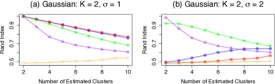
Figure 2: Simulation results for Gaussian clusters with $K=2$, $n=p=30$, averaged over 200 data sets, for two noise levels $\sigma=\{1,2\}$. Colored lines correspond to single linkage hierarchical clustering (), average linkage hierarchical clustering (), $k$-means clustering (), convex clustering with $q=1$ (), and convex clustering with $q=2$ ().

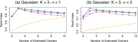
Figure 3: Simulation results for Gaussian clusters with $K=3$, $n=p=30$, averaged over 200 data sets, for two noise levels $\sigma=\{1,2\}$. Line types are as described in Figure 2.

4.2 Non-Convex Clusters

We consider two types of non-convex clusters: two circles clusters (Ng, Jordan and Weiss, 2002) and two half-moon clusters (Hocking et al., 2011; Chi and Lange, 2014a). For two circles clusters, we generate 50 data points from each of the two circles that are centered at $(0,0)$ with radiuses two and 10, respectively. We then add Gaussian random noise with mean zero and standard deviation 0.1 to each data point. For two half-moon clusters, we generate 50 data points from each of the two half-circles that are centered at $(0,0)$ and $(30,3)$ with radius 30, respectively. We then add Gaussian random noise with mean zero and standard deviation one to each data point. Illustrations of both types of clusters are given in Figure 4. The Rand indices for both types of clusters, averaged over 200 data sets, are summarized in Figure 5.

We see from Figure 5 that convex clustering with $q=2$ and single linkage hierarchical clustering have similar performance, and that they outperform all of the other methods. Single linkage hierarchical clustering is able to identify non-convex clusters since it is an agglomerative algorithm that merges the closest pair of observations not yet belonging to the same cluster into one cluster. In contrast, average linkage hierarchical clustering and $k$-means clustering are known to perform poorly on identifying non-convex clusters (Ng, Jordan and Weiss, 2002; Hocking et al., 2011). Again, convex clustering with $q=1$ has the worst performance.

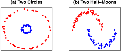
Figure 4: Illustrations of two circles clusters and two half-moons clusters with $n=100$.

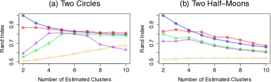
Figure 5: Simulation results for the two circles and two half-moons clusters with $n=100$, averaged over 200 data sets. Line types are as described in Figure 2.

4.3 Selection of the Tuning Parameter $\lambda$

Convex clustering (3) involves a tuning parameter $\lambda$, which determines the estimated number of clusters. Some authors have suggested a hold-out validation approach to select tuning parameters for clustering problems (see, for instance, Tan and Witten, 2014; Chi, Allen and Baraniuk, 2014). In this section, we present an alternative approach for selecting $\lambda$ using the unbiased estimators of the degrees of freedom derived in Section 3.3.

The Bayesian Information Criterion (BIC) developed in Schwarz (1978) has been used extensively for model selection. However, it is known that the BIC does not perform well unless the number of observations is far larger than the number of parameters (Chen and Chen, 2008, 2012). For convex clustering (3), the number of observations is equal to the number of parameters. Thus, we consider the extended BIC (Chen and Chen, 2008, 2012), defined as

$$\mathrm{eBIC}_{q,\gamma}=np\cdot\log\left(\frac{\mathrm{RSS}_{q}}{np}\right)+\hat{\mathrm{df}}_{q}\cdot\log(np)+2\gamma\cdot\hat{\mathrm{df}}_{q}\cdot\log(np),$$ (19)

where $\mathrm{RSS}_{q}=\|\mathbf{x}-\hat{\mathbf{u}}_{q}\|_{2}^{2}$, $\hat{\mathbf{u}}_{q}$ is the convex clustering estimate for a given value of $q$ and $\lambda$, $\gamma\in[0,1]$, and $\hat{\mathrm{df}}_{q}$ is given in Section 3.3. Note that we suppress the dependence of $\hat{\mathbf{u}}_{q}$ and $\hat{\mathrm{df}}_{q}$ on $\lambda$ for notational convenience. We see that when $\gamma=0$, the extended BIC reduces to the classical BIC.

To evaluate the performance of the extended BIC in selecting the number of clusters, we generate Gaussian clusters with $K=2$ and $K=3$ as described in Section 4.1, with $n=p=20$, and $\sigma=0.5$. We perform convex clustering with $q=2$ over a fine grid of $\lambda$, and select the value of $\lambda$ for which the quantity $\mathrm{eBIC}_{q,\gamma}$ is minimized. We consider $\gamma\in\{0,0.5,0.75,1\}$. Table 1 reports the proportion of datasets for which the correct number of clusters was identified, as well as the average Rand index.

From Table 1, we see that the extended BIC is able to select the true number of clusters accurately for $K=2$. When $K=3$, the classical BIC ($\gamma=0$) fails to select the true number of clusters. In contrast, the extended BIC with $\gamma=1$ has the best performance.

Table 1: Simulation study to evaluate the performance of the extended BIC for tuning parameter selection for convex clustering with $q=2$. Results are reported over 100 simulated data sets. We report the proportion of data sets for which the correct number of clusters was identified, and the average Rand index.

	$\mathrm{eBIC}_{2,\gamma}$	Correct number of clusters	Rand index
Gaussian clusters, $K=2$	$\gamma=0$	0.94	0.9896
	$\gamma=0.5$	0.98	0.9991
	$\gamma=0.75$	0.99	0.9995
	$\gamma=1$	0.99	0.9995
Gaussian clusters, $K=3$	$\gamma=0$	0.06	0.7616
	$\gamma=0.5$	0.59	0.9681
	$\gamma=0.75$	0.70	0.9768
	$\gamma=1$	0.84	0.9873

5 Discussion

Convex clustering recasts the clustering problem into a penalized regression problem. By studying its dual problem, we show that there is a connection between convex clustering and single linkage hierarchical clustering. In addition, we establish a connection between convex clustering and $k$-means clustering. We also establish several statistical properties of convex clustering. Through some numerical studies, we illustrate that the performance of convex clustering may not be appealing relative to traditional clustering methods, especially when the signal-to-noise ratio is low.

Many authors have proposed a modification to the convex clustering problem (1),

$$\underset{\mathbf{U}\in\mathbb{R}^{n\times p}}{\mathrm{minimize}}\;\frac{1}{2}\sum_{i=1}^{n}\|\mathbf{X}_{i.}-\mathbf{U}_{i.}\|^{2}_{2}+\lambda\mathrm{Q}_{q}(\mathbf{W},\mathbf{U}),$$ (20)

where $\mathbf{W}$ is an $n\times n$ symmetric matrix of positive weights, and $\mathrm{Q}_{q}(\mathbf{W},\mathbf{U})=\sum_{i<i^{\prime}}W_{ii^{\prime}}\|\mathbf{U}_{i.}-\mathbf{U}_{i^{\prime}.}\|_{q}$ (Pelckmans et al., 2005; Hocking et al., 2011; Lindsten, Ohlsson and Ljung, 2011; Chi and Lange, 2014a). For instance, the weights can be defined as $W_{ii^{\prime}}=\exp\left(-\phi\|\mathbf{X}_{i.}-\mathbf{X}_{i^{\prime}.}\|_{2}^{2}\right)$ for some constant $\phi>0$. This yields better empirical performance than (1) (Hocking et al., 2011; Chi and Lange, 2014a). We leave an investigation of the properties of (20) to future work.

Appendix A: Proof of Lemmas 2—3

Proof of Lemma 2:

Proof.

We rewrite problem (3) as

$$\underset{\mathbf{u}\in\mathbb{R}^{np},\boldsymbol{\eta}_{1}\in\mathbb{R}^{\left[p\cdot{n\choose 2}\right]}}{\mathrm{minimize}}\;\frac{1}{2}\|\mathbf{x-u}\|_{2}^{2}+\lambda\mathrm{P}_{q}(\boldsymbol{\eta}_{1})\quad\quad\text{subject to }\boldsymbol{\eta}_{1}=\mathbf{Du},$$

with the Lagrangian function

$$\mathcal{L}(\mathbf{u},\boldsymbol{\eta}_{1},\boldsymbol{\nu})=\frac{1}{2}\|\mathbf{x}-\mathbf{u}\|_{2}^{2}+\lambda\mathrm{P}_{q}(\boldsymbol{\eta}_{1})+\boldsymbol{\nu}^{T}(\mathbf{Du}-\boldsymbol{\eta}_{1}),$$ (A-1)

where $\boldsymbol{\nu}\in\mathbb{R}^{\left[p\cdot{n\choose 2}\right]}$ is the Lagrangian dual variable. In order to derive the dual problem, we need to minimize the Lagrangian function over the primal variables $\mathbf{u}$ and $\boldsymbol{\eta}_{1}$. Recall from (4) that $\mathrm{P}^{*}_{q}(\cdot)$ is the dual norm of $\mathrm{P}_{q}(\cdot)$. It can be shown that

$$\underset{\boldsymbol{\eta}_{1}\in\mathbb{R}^{\left[p\cdot{n\choose 2}\right]}}{\mathrm{inf}}\;\mathcal{L}(\mathbf{u},\boldsymbol{\eta}_{1},\boldsymbol{\nu})=\begin{cases}\frac{1}{2}\|\mathbf{x}-\mathbf{u}\|_{2}^{2}+\boldsymbol{\nu}^{T}\mathbf{Du}&\text{if}\quad\mathrm{P}^{*}_{q}(\boldsymbol{\nu})\leq\lambda,\\ -\infty&\mathrm{otherwise,}\end{cases}$$

and

$$\underset{\boldsymbol{\eta}_{1}\in\mathbb{R}^{\left[p\cdot{n\choose 2}\right]},\mathbf{u}\in\mathbb{R}^{np}}{\mathrm{inf}}\;\mathcal{L}(\mathbf{u},\boldsymbol{\eta}_{1},\boldsymbol{\nu})=\begin{cases}-\frac{1}{2}\|\mathbf{x}-\mathbf{D}^{T}\boldsymbol{\nu}\|_{2}^{2}+\frac{1}{2}\|\mathbf{x}\|_{2}^{2}&\text{if}\quad\mathrm{P}^{*}_{q}(\boldsymbol{\nu})\leq\lambda.\\ -\infty&\mathrm{otherwise.}\end{cases}$$

Therefore, the dual problem for (3) is

$$\underset{\boldsymbol{\nu}\in\mathbb{R}^{\left[p\cdot{n\choose 2}\right]}}{\mathrm{minimize}}\;\frac{1}{2}\|\mathbf{x}-\mathbf{D}^{T}\boldsymbol{\nu}\|_{2}^{2}\quad\quad\mathrm{subject\;to}\;\mathrm{P}^{*}_{q}(\boldsymbol{\nu})\leq\lambda.$$ (A-2)

We now establish an explicit relationship between the solution to convex clustering and its dual problem. Differentiating the Lagrangian function (A-1) with respect to $\mathbf{u}$ and setting it equal to zero, we obtain

$$\hat{\mathbf{u}}=\mathbf{x}-\mathbf{D}^{T}\hat{\boldsymbol{\nu}},$$

where $\hat{\boldsymbol{\nu}}$ is the solution to the dual problem, which satisfies $\mathrm{P}_{q}^{*}(\hat{\boldsymbol{\nu}})\leq\lambda$ by (A-2). Multiplying both sides by $\mathbf{D}$, we obtain the relationship (6). ∎

Proof of Lemma 3:

Proof.

We rewrite (7) as

$$\underset{\boldsymbol{\gamma}\in\mathbb{R}^{\left[p\cdot{n\choose 2}\right]},\boldsymbol{\eta}_{2}\in\mathbb{R}^{\left[p\cdot{n\choose 2}\right]}}{\mathrm{minimize}}\;\frac{1}{2}\|\mathbf{Dx}-\boldsymbol{\gamma}\|_{2}^{2}+\lambda\mathrm{P}_{q}(\boldsymbol{\eta}_{2})\qquad\text{subject to }\boldsymbol{\eta}_{2}=\boldsymbol{\gamma},$$

with the Lagrangian function

$$\mathcal{L}(\boldsymbol{\gamma},\boldsymbol{\eta}_{2},\boldsymbol{\nu}^{\prime})=\frac{1}{2}\|\mathbf{Dx}-\boldsymbol{\gamma}\|_{2}^{2}+\lambda\mathrm{P}_{q}(\boldsymbol{\eta}_{2})+(\boldsymbol{\nu}^{\prime})^{T}(\boldsymbol{\gamma}-\boldsymbol{\eta}_{2}),$$ (A-3)

where $\boldsymbol{\nu}^{\prime}\in\mathbb{R}^{\left[p\cdot{n\choose 2}\right]}$ is the Lagrangian dual variable. In order to derive the dual problem, we minimize the Lagrangian function over the primal variables $\boldsymbol{\gamma}$ and $\boldsymbol{\eta}_{2}$. It can be shown that

$$\underset{\boldsymbol{\eta}_{2}\in\mathbb{R}^{\left[p\cdot{n\choose 2}\right]}}{\mathrm{inf}}\;\mathcal{L}(\boldsymbol{\gamma},\boldsymbol{\eta}_{2},\boldsymbol{\nu}^{\prime})=\begin{cases}\frac{1}{2}\|\mathbf{Dx}-\boldsymbol{\gamma}\|_{2}^{2}+(\boldsymbol{\nu}^{\prime})^{T}\boldsymbol{\gamma}&\text{if}\quad\mathrm{P}^{*}_{q}(\boldsymbol{\nu}^{\prime})\leq\lambda,\\ -\infty&\mathrm{otherwise,}\end{cases}$$

and

$$\underset{\boldsymbol{\eta}_{2}\in\mathbb{R}^{\left[p\cdot{n\choose 2}\right]},\boldsymbol{\gamma}\in\mathbb{R}^{\left[p\cdot{n\choose 2}\right]}}{\mathrm{inf}}\;\mathcal{L}(\boldsymbol{\gamma},\boldsymbol{\eta}_{2},\boldsymbol{\nu}^{\prime})=\begin{cases}-\frac{1}{2}\|\mathbf{Dx}-\boldsymbol{\nu}^{\prime}\|_{2}^{2}+\frac{1}{2}\|\mathbf{Dx}\|_{2}^{2}&\text{if}\quad\mathrm{P}^{*}_{q}(\boldsymbol{\nu}^{\prime})\leq\lambda.\\ -\infty&\mathrm{otherwise.}\end{cases}$$

Therefore, the dual problem for (7) is

$$\underset{\boldsymbol{\nu}^{\prime}\in\mathbb{R}^{\left[p\cdot{n\choose 2}\right]}}{\mathrm{minimize}}\;\frac{1}{2}\|\mathbf{Dx}-\boldsymbol{\nu}^{\prime}\|_{2}^{2}\quad\quad\text{subject to }\mathrm{P}^{*}_{q}(\boldsymbol{\nu}^{\prime})\leq\lambda.$$ (A-4)

We now establish an explicit relationship between the solution to (7) and its dual problem. Differentiating the Lagrangian function (A-3) with respect to $\boldsymbol{\gamma}$ and setting it equal to zero, we obtain

$$\hat{\boldsymbol{\gamma}}=\mathbf{Dx}-\hat{\boldsymbol{\nu}}^{\prime},$$

where $\hat{\boldsymbol{\nu}}^{\prime}$ is the solution to the dual problem, which we know from (A-4) satisfies $\mathrm{P}_{q}^{*}(\hat{\boldsymbol{\nu}}^{\prime})\leq\lambda$. ∎

Appendix B: Proof of Lemma 5

Proof of Lemma 5:

Proof.

Since $\mathbf{D}$ is not of full rank by Lemma 1(i), the solution to (5) in the absence of constraint is not unique, and takes the form

$$\begin{split}\hat{\boldsymbol{\nu}}&=(\mathbf{DD}^{T})^{\dagger}\mathbf{Dx}+(\mathbf{I}-\mathbf{D}(\mathbf{D}^{T}\mathbf{D})^{\dagger}\mathbf{D}^{T})\boldsymbol{\omega}\\ &=(\mathbf{D}^{T})^{\dagger}\mathbf{x}+(\mathbf{I}-\mathbf{DD}^{\dagger})\boldsymbol{\omega}\\ &=\frac{1}{n}\mathbf{Dx}+(\mathbf{I}-\frac{1}{n}\mathbf{D}\mathbf{D}^{T})\boldsymbol{\omega},\end{split}$$ (B-1)

for $\boldsymbol{\omega}\in\mathbb{R}^{\left[p\cdot{n\choose 2}\right]}$. The second equality follows from Lemma 1(iii) and the last equality follows from Lemma 1(ii).

Let $\hat{\mathbf{u}}$ be the solution to (3). Substituting $\hat{\boldsymbol{\nu}}$ given in (B-1) into (6), we obtain

$$\begin{split}\mathbf{D}\hat{\mathbf{u}}&=\mathbf{Dx}-\mathbf{DD}^{T}\hat{\boldsymbol{\nu}}\\ &=\mathbf{Dx}-\frac{1}{n}\mathbf{DD}^{T}\mathbf{Dx}-\mathbf{DD}^{T}\boldsymbol{\omega}+\frac{1}{n}\mathbf{DD}^{T}\mathbf{DD}^{T}\boldsymbol{\omega}\\ &=\mathbf{Dx}-\mathbf{Dx}-\mathbf{DD}^{T}\boldsymbol{\omega}+\mathbf{DD}^{T}\boldsymbol{\omega}\\ &=\mathbf{0}.\end{split}$$

Recall from Definition 1 that all observations are estimated to belong to the same cluster if $\mathbf{D}\hat{\mathbf{u}}=\mathbf{0}$. For any $\hat{\boldsymbol{\nu}}$ in (B-1), picking $\lambda=\mathrm{P}^{*}_{q}(\hat{\boldsymbol{\nu}})$ guarantees that the constraint on the dual problem (5) is inactive, and therefore that convex clustering has a trivial solution of $\mathbf{D}\hat{\mathbf{u}}=\mathbf{0}$.

Since $\hat{\boldsymbol{\nu}}$ is not unique, $\mathrm{P}^{*}_{q}(\hat{\boldsymbol{\nu}})$ is not unique. In order to obtain the smallest tuning parameter $\lambda$ such that $\mathbf{D}\hat{\mathbf{u}}=\mathbf{0}$, we take

$$\lambda_{\mathrm{upper}}:=\underset{\boldsymbol{\omega}\in\mathbb{R}^{\left[p\cdot{n\choose 2}\right]}}{\min}\mathrm{P}^{*}_{q}\left(\frac{1}{n}\mathbf{Dx}+\left(\mathbf{I}-\frac{1}{n}\mathbf{D}\mathbf{D}^{T}\right){\boldsymbol{\omega}}\right).$$

Any tuning parameter $\lambda\geq\lambda_{\mathrm{upper}}$ results in an estimate for which all observations belong to a single cluster. The proof is completed by recalling the definition of the dual norm $\mathrm{P}_{q}^{*}(\cdot)$ in (4). ∎

Appendix C: Proof of Lemmas 6—7

To prove Lemmas 6 and 7, we need a lemma on the tail bound for quadratic forms of independent sub-Gaussian random variables.

Lemma 10.

(Hanson and Wright, 1971) Let $\mathbf{z}$ be a vector of independent sub-Gaussian random variables with mean zero and variance $\sigma^{2}$. Let $\mathbf{M}$ be a symmetric matrix. Then, there exists some constants $c_{1},c_{2}>0$ such that for any $t>0$,

$$\mathrm{Pr}\left(\mathbf{z}^{T}\mathbf{Mz}\geq t+\sigma^{2}\mathrm{tr}(\mathbf{M})\right)\leq\exp\left\{-\min\left(\frac{c_{1}t^{2}}{\sigma^{4}\|\mathbf{M}\|_{\mathrm{F}}},\frac{c_{2}t}{\sigma^{2}\|\mathbf{M}\|_{\mathrm{sp}}}\right)\right\},$$

where $\|\cdot\|_{\mathrm{F}}$ and $\|\cdot\|_{\mathrm{sp}}$ are the Frobenius norm and spectral norm, respectively.

In order to simplify our analysis, we start by reformulating (3) as in Liu, Yuan and Ye (2013). Let $\mathbf{D}=\mathbf{A}\Lambda\mathbf{V}_{\beta}^{T}$ be the singular value decomposition of $\mathbf{D}$, where $\mathbf{A}\in\mathbb{R}^{\left[p\cdot{n\choose 2}\right]\times p(n-1)}$, $\Lambda\in\mathbb{R}^{p(n-1)\times p(n-1)}$, and $\mathbf{V}_{\beta}\in\mathbb{R}^{np\times p(n-1)}$. Construct $\mathbf{V}_{\alpha}\in\mathbb{R}^{np\times p}$ such that $\mathbf{V}=[\mathbf{V}_{\alpha},\mathbf{V}_{\beta}]\in\mathbb{R}^{np\times np}$ is an orthogonal matrix, that is, $\mathbf{V}^{T}\mathbf{V}=\mathbf{VV}^{T}=\mathbf{I}$. Note that $\mathbf{V}_{\alpha}^{T}\mathbf{V}_{\beta}=0$.

Let $\boldsymbol{\beta}=\mathbf{V}_{\beta}^{T}\mathbf{u}\in\mathbb{R}^{p(n-1)}$ and $\boldsymbol{\alpha}=\mathbf{V}_{\alpha}^{T}\mathbf{u}\in\mathbb{R}^{p}$. Also, let $\lambda^{\prime}=\frac{\lambda}{np}$. Optimization problem (3) then becomes

$$\underset{\boldsymbol{\alpha}\in\mathbb{R}^{p},\boldsymbol{\beta}\in\mathbb{R}^{p(n-1)}}{\mathrm{minimize}}\;\frac{1}{2np}\|\mathbf{x}-\mathbf{V}_{\alpha}\boldsymbol{\alpha}-\mathbf{V}_{\beta}\boldsymbol{\beta}\|^{2}+\lambda^{\prime}\mathrm{P}_{q}(\mathbf{Z}\boldsymbol{\beta}),$$ (C-1)

where $\mathbf{Z}=\mathbf{A}\Lambda\in\mathbb{R}^{\left[p\cdot{n\choose 2}\right]\times p(n-1)}$. Note that $\mathrm{rank}(\mathbf{Z})=p(n-1)$ and therefore, there exists a pseudo-inverse $\mathbf{Z}^{\dagger}\in\mathbb{R}^{p(n-1)\times\left[p\cdot{n\choose 2}\right]}$ such that $\mathbf{Z}^{\dagger}\mathbf{Z}=\mathbf{I}$. Recall from Section 1 that the set $\mathcal{C}(i,i^{\prime})$ contains the row indices of $\mathbf{D}$ such that $\mathbf{D}_{\mathcal{C}(i,i^{\prime})}\mathbf{u}=\mathbf{U}_{i.}-\mathbf{U}_{i^{\prime}.}$. Let the submatrices $\mathbf{Z}_{\mathcal{C}{(i,i^{\prime})}}$ and $\mathbf{Z}^{\dagger}_{\mathcal{C}(i,i^{\prime})}$ denote the rows of $\mathbf{Z}$ and the columns of $\mathbf{Z}^{\dagger}$, respectively, corresponding to the indices in the set $\mathcal{C}(i,i^{\prime})$. By Lemma 1(v),

$$\small\Lambda_{\min}(\mathbf{Z})=\Lambda_{\min}(\mathbf{D})=\frac{1}{\Lambda_{\max}(\mathbf{Z}^{\dagger})}=\sqrt{n}\qquad\text{and}\qquad\Lambda_{\max}(\mathbf{Z})=\Lambda_{\max}(\mathbf{D})=\frac{1}{\Lambda_{\min}(\mathbf{Z}^{\dagger})}=\sqrt{n}.$$ (C-2)

Let $\hat{\boldsymbol{\alpha}}$ and $\hat{\boldsymbol{\beta}}$ denote the solution to (C-1).

Proof of Lemma 6:

Proof.

We establish a finite sample bound for the prediction error of convex clustering with $q=1$ by analyzing (C-1). First, note that $\hat{\mathbf{u}}=\mathbf{V}_{\alpha}\hat{\boldsymbol{\alpha}}+\mathbf{V}_{\beta}\hat{\boldsymbol{\beta}}$ and ${\mathbf{u}}=\mathbf{V}_{\alpha}{\boldsymbol{\alpha}}+\mathbf{V}_{\beta}{\boldsymbol{\beta}}$. Thus, $\frac{1}{2np}\|\hat{\mathbf{u}}-\mathbf{u}\|^{2}=\frac{1}{2np}\|\mathbf{V}_{\alpha}(\hat{\boldsymbol{\alpha}}-\boldsymbol{\alpha})+\mathbf{V}_{\beta}(\hat{\boldsymbol{\beta}}-\boldsymbol{\beta})\|^{2}$. Recall from (2) that $\mathrm{P}_{1}(\mathbf{Z}\boldsymbol{\beta})=\|\mathbf{Z}\boldsymbol{\beta}\|_{1}$. By the definition of $\hat{\boldsymbol{\alpha}}$ and $\hat{\boldsymbol{\beta}}$, we have

$$\frac{1}{2np}\|\mathbf{x}-(\mathbf{V}_{\alpha}\hat{\boldsymbol{\alpha}}+\mathbf{V}_{\beta}\hat{\boldsymbol{\beta}})\|^{2}+\lambda^{\prime}\|\mathbf{Z}\hat{\boldsymbol{\beta}}\|_{1}\leq\frac{1}{2np}\|\mathbf{x}-(\mathbf{V}_{\alpha}\boldsymbol{\alpha}+\mathbf{V}_{\beta}\boldsymbol{\beta})\|^{2}+\lambda^{\prime}\|\mathbf{Z}\boldsymbol{\beta}\|_{1},$$

implying

$$\frac{1}{2np}\|\mathbf{V}_{\alpha}(\hat{\boldsymbol{\alpha}}-\boldsymbol{\alpha})+\mathbf{V}_{\beta}(\hat{\boldsymbol{\beta}}-\boldsymbol{\beta})\|^{2}+\lambda^{\prime}\|\mathbf{Z}\hat{\boldsymbol{\beta}}\|_{1}\leq\frac{1}{np}\mathrm{G}(\hat{\boldsymbol{\alpha}},\hat{\boldsymbol{\beta}})+\lambda^{\prime}\|\mathbf{Z}\boldsymbol{\beta}\|_{1},$$ (C-3)

where $\mathrm{G}(\hat{\boldsymbol{\alpha}},\hat{\boldsymbol{\beta}})=\boldsymbol{\epsilon}^{T}\left[\mathbf{V}_{\alpha}(\hat{\boldsymbol{\alpha}}-\boldsymbol{\alpha})+\mathbf{V}_{\beta}(\hat{\boldsymbol{\beta}}-\boldsymbol{\beta})\right]$. Recall that $\mathbf{V}_{\alpha}^{T}\mathbf{V}_{\alpha}=\mathbf{I}$ and $\mathbf{V}_{\alpha}^{T}\mathbf{V}_{\beta}=\mathbf{0}$. By the optimality condition of (C-1),

$$\begin{split}\hat{\boldsymbol{\alpha}}&=\mathbf{V}_{\alpha}^{T}(\mathbf{x}-\mathbf{V}_{\beta}\hat{\boldsymbol{\beta}})\\ &=\mathbf{V}_{\alpha}^{T}\left(\mathbf{V}_{\alpha}\boldsymbol{\alpha}+\mathbf{V}_{\beta}\boldsymbol{\beta}+\boldsymbol{\epsilon}-\mathbf{V}_{\beta}\hat{\boldsymbol{\beta}}\right)\\ &=\boldsymbol{\alpha}+\mathbf{V}^{T}_{\alpha}\boldsymbol{\epsilon}.\end{split}$$

Therefore, substituting $\hat{\boldsymbol{\alpha}}-\boldsymbol{\alpha}=\mathbf{V}^{T}_{\alpha}\boldsymbol{\epsilon}$ into $\mathrm{G}(\hat{\boldsymbol{\alpha}},\hat{\boldsymbol{\beta}})$, we obtain

$$\small\begin{split}\frac{1}{np}\left|\mathrm{G}(\hat{\boldsymbol{\alpha}},\hat{\boldsymbol{\beta}})\right|&=\frac{1}{np}\left|\boldsymbol{\epsilon}^{T}\left[\mathbf{V}_{\alpha}(\hat{\boldsymbol{\alpha}}-\boldsymbol{\alpha})+\mathbf{V}_{\beta}(\hat{\boldsymbol{\beta}}-\boldsymbol{\beta})\right]\right|\\ &=\frac{1}{np}\left|\boldsymbol{\epsilon}^{T}\mathbf{V}_{\alpha}\mathbf{V}^{T}_{\alpha}\boldsymbol{\epsilon}+\boldsymbol{\epsilon}^{T}\mathbf{V}_{\beta}(\hat{\boldsymbol{\beta}}-\boldsymbol{\beta})\right|\\ &\leq\frac{1}{np}\boldsymbol{\epsilon}^{T}\mathbf{V}_{\alpha}\mathbf{V}_{\alpha}^{T}\boldsymbol{\epsilon}+\frac{1}{np}\left|\boldsymbol{\epsilon}^{T}\mathbf{V}_{\beta}(\hat{\boldsymbol{\beta}}-\boldsymbol{\beta})\right|\\ &=\frac{1}{np}\boldsymbol{\epsilon}^{T}\mathbf{V}_{\alpha}\mathbf{V}_{\alpha}^{T}\boldsymbol{\epsilon}+\frac{1}{np}\left|\boldsymbol{\epsilon}^{T}\mathbf{V}_{\beta}\mathbf{Z}^{\dagger}\mathbf{Z}(\hat{\boldsymbol{\beta}}-\boldsymbol{\beta})\right|\\ &\leq\frac{1}{np}\boldsymbol{\epsilon}^{T}\mathbf{V}_{\alpha}\mathbf{V}_{\alpha}^{T}\boldsymbol{\epsilon}+\frac{1}{np}\|\boldsymbol{\epsilon}^{T}\mathbf{V}_{\beta}\mathbf{Z}^{\dagger}\|_{\infty}\|\mathbf{Z}(\hat{\boldsymbol{\beta}}-\boldsymbol{\beta})\|_{1}.\\ \end{split}$$

We now establish bounds for $\frac{1}{np}\boldsymbol{\epsilon}^{T}\mathbf{V}_{\alpha}\mathbf{V}_{\alpha}^{T}\boldsymbol{\epsilon}$ and $\frac{1}{np}\|\boldsymbol{\epsilon}^{T}\mathbf{V}_{\beta}\mathbf{Z}^{\dagger}\|_{\infty}$ that hold with high probability.

Bound for $\frac{1}{np}\boldsymbol{\epsilon}^{T}\mathbf{V}_{\alpha}\mathbf{V}_{\alpha}^{T}\boldsymbol{\epsilon}$:

First, note that $\mathbf{V}_{\alpha}\mathbf{V}_{\alpha}^{T}$ is a projection matrix of rank $p$, and therefore $\|\mathbf{V}_{\alpha}\mathbf{V}_{\alpha}^{T}\|_{\mathrm{sp}}=1$ and $\|\mathbf{V}_{\alpha}\mathbf{V}_{\alpha}^{T}\|_{\mathrm{F}}=p$. By Lemma 10 and taking $\mathbf{z}=\boldsymbol{\epsilon}$ and $\mathbf{M}=\mathbf{V}_{\alpha}\mathbf{V}_{\alpha}^{T}$, we have that

$$\mathrm{Pr}\left(\boldsymbol{\epsilon}^{T}\mathbf{V}_{\alpha}\mathbf{V}_{\alpha}^{T}\boldsymbol{\epsilon}\geq t+\sigma^{2}p\right)\leq\exp\left\{-\min\left(\frac{c_{1}t^{2}}{\sigma^{4}p},\frac{c_{2}t}{\sigma^{2}}\right)\right\},$$

where $c_{1}$ and $c_{2}$ are constants in Lemma 10. Picking $t=\sigma^{2}\sqrt{p\log(np)}$, we have

$$\mathrm{Pr}\left(\frac{1}{np}\boldsymbol{\epsilon}^{T}\mathbf{V}_{\alpha}\mathbf{V}_{\alpha}^{T}\boldsymbol{\epsilon}\geq\sigma^{2}\left[\frac{1}{n}+\sqrt{\frac{\log(np)}{n^{2}p}}\right]\right)\leq\exp\left\{-\min\left(c_{1}\log(np),c_{2}\sqrt{p\log(np)}\right)\right\}.$$ (C-4)

Bound for $\frac{1}{np}\|\boldsymbol{\epsilon}^{T}\mathbf{V}_{\beta}\mathbf{Z}^{\dagger}\|_{\infty}$:

Let $e_{j}$ be a vector of length $p\cdot{n\choose 2}$ with a one in the $j$th entry and zeroes in the remaining entries. Let $v_{j}=e_{j}^{T}(\mathbf{Z}^{\dagger})^{T}\mathbf{V}_{\beta}^{T}\boldsymbol{\epsilon}$. Using the fact that $\Lambda_{\max}(\mathbf{V}_{\beta})=1$ and $\Lambda_{\max}(\mathbf{Z}^{\dagger})=\frac{1}{\sqrt{n}}$ (C-2), we know that each $v_{j}$ is a sub-Gaussian random variable with zero mean and variance at most $\frac{\sigma^{2}}{n}$. Therefore, by the union bound,

$$\mathrm{Pr}\left(\underset{j}{\max}\;|v_{j}|\geq z\right)\leq p\cdot{n\choose 2}\cdot\mathrm{Pr}\left(|v_{j}|\geq z\right)\leq 2p\cdot{n\choose 2}\exp\left(-\frac{nz^{2}}{2\sigma^{2}}\right).$$

Picking $z=2\sigma\sqrt{\frac{\log\left(p\cdot{n\choose 2}\right)}{n}}$, we obtain

$$\mathrm{Pr}\left(\|\boldsymbol{\epsilon}^{T}\mathbf{V}_{\beta}\mathbf{Z}^{\dagger}\|_{\infty}\geq 2\sigma\sqrt{\frac{\log(p\cdot{n\choose 2})}{n}}\right)\leq\frac{2}{p\cdot{n\choose 2}}.$$ (C-5)

Combining the two upper bounds: Setting $\lambda^{\prime}>4\sigma\sqrt{\frac{\log\left(p\cdot{n\choose 2}\right)}{n^{3}p^{2}}}$ and combining the results from (C-4) and (C-5), we obtain

$$\frac{1}{np}\mathrm{G}(\hat{\boldsymbol{\alpha}},\hat{\boldsymbol{\beta}})\leq\sigma^{2}\left[\frac{1}{n}+\sqrt{\frac{\log(np)}{n^{2}p}}\right]+\frac{\lambda^{\prime}}{2}\|\mathbf{Z}(\hat{\boldsymbol{\beta}}-\boldsymbol{\beta})\|_{1}$$ (C-6)

with probability at least $1-\frac{2}{p\cdot{n\choose 2}}-\exp\left\{-\min\left(c_{1}\log(np),c_{2}\sqrt{p\log(np)}\right)\right\}$. Substituting (C-6) into (C-3), we obtain

$$\small\begin{split}&\quad\frac{1}{2np}\|\mathbf{V}_{\alpha}(\hat{\boldsymbol{\alpha}}-\boldsymbol{\alpha})+\mathbf{V}_{\beta}(\hat{\boldsymbol{\beta}}-\boldsymbol{\beta})\|^{2}+\lambda^{\prime}\|\mathbf{Z}\hat{\boldsymbol{\beta}}\|_{1}\\ &\leq\sigma^{2}\left[\frac{1}{n}+\sqrt{\frac{\log(np)}{n^{2}p}}\right]+\frac{\lambda^{\prime}}{2}\|\mathbf{Z}(\hat{\boldsymbol{\beta}}-\boldsymbol{\beta})\|_{1}+\lambda^{\prime}\|\mathbf{Z}\boldsymbol{\beta}\|_{1}.\end{split}$$

We get Lemma 6 by an application of the triangle inequality and by rearranging the terms. ∎

Proof of Lemma 7:

Proof.

We establish a finite sample bound for the prediction error of convex clustering with $q=2$ by analyzing (C-1). Recall from (2) that $\mathrm{P}_{2}(\mathbf{Z}\boldsymbol{\beta})=\sum_{i<i^{\prime}}\|\mathbf{Z}_{\mathcal{C}(i,i^{\prime})}\boldsymbol{\beta}\|_{2}$. By the definition of $\hat{\boldsymbol{\alpha}}$ and $\hat{\boldsymbol{\beta}}$, we have

$$\frac{1}{2np}\|\mathbf{x}-(\mathbf{V}_{\alpha}\hat{\boldsymbol{\alpha}}+\mathbf{V}_{\beta}\hat{\boldsymbol{\beta}})\|^{2}+\lambda^{\prime}\sum_{i<i^{\prime}}\|\mathbf{Z}_{\mathcal{C}(i,i^{\prime})}\hat{\boldsymbol{\beta}}\|_{2}\leq\frac{1}{2np}\|\mathbf{x}-(\mathbf{V}_{\alpha}\boldsymbol{\alpha}+\mathbf{V}_{\beta}\boldsymbol{\beta})\|^{2}+\lambda^{\prime}\sum_{i<i^{\prime}}\|\mathbf{Z}_{\mathcal{C}(i,i^{\prime})}\boldsymbol{\beta}\|_{2},$$

implying

$$\frac{1}{2np}\|\mathbf{V}_{\alpha}(\hat{\boldsymbol{\alpha}}-\boldsymbol{\alpha})+\mathbf{V}_{\beta}(\hat{\boldsymbol{\beta}}-\boldsymbol{\beta})\|^{2}+\lambda^{\prime}\sum_{i<i^{\prime}}\|\mathbf{Z}_{\mathcal{C}(i,i^{\prime})}\hat{\boldsymbol{\beta}}\|_{2}\leq\frac{1}{np}\mathrm{G}(\hat{\boldsymbol{\alpha}},\hat{\boldsymbol{\beta}})+\lambda^{\prime}\sum_{i<i^{\prime}}\|\mathbf{Z}_{\mathcal{C}(i,i^{\prime})}\boldsymbol{\beta}\|_{2},$$ (C-7)

where $\mathrm{G}(\hat{\boldsymbol{\alpha}},\hat{\boldsymbol{\beta}})=\boldsymbol{\epsilon}^{T}\left[\mathbf{V}_{\alpha}(\hat{\boldsymbol{\alpha}}-\boldsymbol{\alpha})+\mathbf{V}_{\beta}(\hat{\boldsymbol{\beta}}-\boldsymbol{\beta})\right]$. Again, by the optimality condition of (C-1), we have that $\hat{\boldsymbol{\alpha}}-\boldsymbol{\alpha}=\mathbf{V}^{T}_{\alpha}\boldsymbol{\epsilon}$. Substituting this into $\frac{1}{np}\mathrm{G}(\hat{\boldsymbol{\alpha}},\hat{\boldsymbol{\beta}})$, we obtain

$$\small\begin{split}\frac{1}{np}\left|\mathrm{G}(\hat{\boldsymbol{\alpha}},\hat{\boldsymbol{\beta}})\right|&=\frac{1}{np}\left|\boldsymbol{\epsilon}^{T}\left[\mathbf{V}_{\alpha}(\hat{\boldsymbol{\alpha}}-\boldsymbol{\alpha})+\mathbf{V}_{\beta}(\hat{\boldsymbol{\beta}}-\boldsymbol{\beta})\right]\right|\\ &=\frac{1}{np}\left|\boldsymbol{\epsilon}^{T}\mathbf{V}_{\alpha}\mathbf{V}^{T}_{\alpha}\boldsymbol{\epsilon}+\boldsymbol{\epsilon}^{T}\mathbf{V}_{\beta}(\hat{\boldsymbol{\beta}}-\boldsymbol{\beta})\right|\\ &\leq\frac{1}{np}\boldsymbol{\epsilon}^{T}\mathbf{V}_{\alpha}\mathbf{V}_{\alpha}^{T}\boldsymbol{\epsilon}+\frac{1}{np}\left|\boldsymbol{\epsilon}^{T}\mathbf{V}_{\beta}(\hat{\boldsymbol{\beta}}-\boldsymbol{\beta})\right|\\ &=\frac{1}{np}\boldsymbol{\epsilon}^{T}\mathbf{V}_{\alpha}\mathbf{V}_{\alpha}^{T}\boldsymbol{\epsilon}+\frac{1}{np}\left|\boldsymbol{\epsilon}^{T}\mathbf{V}_{\beta}\mathbf{Z}^{\dagger}\mathbf{Z}(\hat{\boldsymbol{\beta}}-\boldsymbol{\beta})\right|\\ &=\frac{1}{np}\boldsymbol{\epsilon}^{T}\mathbf{V}_{\alpha}\mathbf{V}_{\alpha}^{T}\boldsymbol{\epsilon}+\frac{1}{np}\left|\sum_{i<i^{\prime}}(\boldsymbol{\epsilon}^{T}\mathbf{V}_{\beta}\mathbf{Z}_{\mathcal{C}(i,i^{\prime})}^{\dagger})(\mathbf{Z}_{\mathcal{C}(i,i^{\prime})}(\hat{\boldsymbol{\beta}}-\boldsymbol{\beta}))\right|\\ &\leq\frac{1}{np}\boldsymbol{\epsilon}^{T}\mathbf{V}_{\alpha}\mathbf{V}_{\alpha}^{T}\boldsymbol{\epsilon}+\frac{1}{np}\sum_{i<i^{\prime}}\left|(\boldsymbol{\epsilon}^{T}\mathbf{V}_{\beta}\mathbf{Z}_{\mathcal{C}(i,i^{\prime})}^{\dagger})(\mathbf{Z}_{\mathcal{C}(i,i^{\prime})}(\hat{\boldsymbol{\beta}}-\boldsymbol{\beta}))\right|\\ &\leq\frac{1}{np}\boldsymbol{\epsilon}^{T}\mathbf{V}_{\alpha}\mathbf{V}_{\alpha}^{T}\boldsymbol{\epsilon}+\frac{1}{np}\sum_{i<i^{\prime}}\|\boldsymbol{\epsilon}^{T}\mathbf{V}_{\beta}\mathbf{Z}_{\mathcal{C}(i,i^{\prime})}^{\dagger}\|_{2}\|\mathbf{Z}_{\mathcal{C}(i,i^{\prime})}(\hat{\boldsymbol{\beta}}-\boldsymbol{\beta})\|_{2}\\ &\leq\frac{1}{np}\boldsymbol{\epsilon}^{T}\mathbf{V}_{\alpha}\mathbf{V}_{\alpha}^{T}\boldsymbol{\epsilon}+\frac{1}{np}\cdot\underset{i<i^{\prime}}{\max}\;\|\boldsymbol{\epsilon}^{T}\mathbf{V}_{\beta}\mathbf{Z}^{\dagger}_{\mathcal{C}(i,i^{\prime})}\|_{2}\sum_{i<i^{\prime}}\|\mathbf{Z}_{\mathcal{C}(i,i^{\prime})}(\hat{\boldsymbol{\beta}}-\boldsymbol{\beta})\|_{2},\\ \end{split}$$

where the second inequality follows from an application of the triangle inequality and the third inequality from an application of the Cauchy-Schwarz inequality. We now establish bounds for $\frac{1}{np}\boldsymbol{\epsilon}^{T}\mathbf{V}_{\alpha}\mathbf{V}_{\alpha}^{T}\boldsymbol{\epsilon}$ and $\frac{1}{np}\cdot\underset{i<i^{\prime}}{\max}\;\|\boldsymbol{\epsilon}^{T}\mathbf{V}_{\beta}\mathbf{Z}^{\dagger}_{\mathcal{C}(i,i^{\prime})}\|_{2}$ that hold with large probability.

Bound for $\frac{1}{np}\boldsymbol{\epsilon}^{T}\mathbf{V}_{\alpha}\mathbf{V}_{\alpha}^{T}\boldsymbol{\epsilon}$:

This is established in the proof of Lemma 6 in (C-4), i.e.,

$$\mathrm{Pr}\left(\frac{1}{np}\boldsymbol{\epsilon}^{T}\mathbf{V}_{\alpha}\mathbf{V}_{\alpha}^{T}\boldsymbol{\epsilon}\geq\sigma^{2}\left[\frac{1}{n}+\sqrt{\frac{\log(np)}{n^{2}p}}\right]\right)\leq\frac{1}{np}.$$

Bound for $\frac{1}{np}\cdot\underset{i<i^{\prime}}{\max}\;\|\boldsymbol{\epsilon}^{T}\mathbf{V}_{\beta}\mathbf{Z}^{\dagger}_{\mathcal{C}(i,i^{\prime})}\|_{2}$:

First, note that there are $p$ indices in each set $\mathcal{C}(i,i^{\prime})$. Therefore,

$$\|\boldsymbol{\epsilon}^{T}\mathbf{V}_{\beta}\mathbf{Z}^{\dagger}_{\mathcal{C}(i,i^{\prime})}\|_{2}\leq\sqrt{p}\cdot\|\boldsymbol{\epsilon}^{T}\mathbf{V}_{\beta}\mathbf{Z}^{\dagger}_{\mathcal{C}(i,i^{\prime})}\|_{\infty}.$$

Note that

$$\frac{1}{np}\cdot\underset{i<i^{\prime}}{\max}\;\|\boldsymbol{\epsilon}^{T}\mathbf{V}_{\beta}\mathbf{Z}^{\dagger}_{\mathcal{C}(i,i^{\prime})}\|_{2}\leq\sqrt{\frac{1}{n^{2}p}}\cdot\underset{i<i^{\prime}}{\max}\;\|\boldsymbol{\epsilon}^{T}\mathbf{V}_{\beta}\mathbf{Z}^{\dagger}_{\mathcal{C}(i,i^{\prime})}\|_{\infty}=\sqrt{\frac{1}{n^{2}p}}\cdot\|\boldsymbol{\epsilon}^{T}\mathbf{V}_{\beta}\mathbf{Z}^{\dagger}\|_{\infty}.$$ (C-8)

Therefore, using (C-8),

$$\begin{split}&\quad\;\mathrm{Pr}\left(\frac{1}{np}\cdot\underset{i<i^{\prime}}{\max}\;\|\boldsymbol{\epsilon}^{T}\mathbf{V}_{\beta}\mathbf{Z}^{\dagger}_{\mathcal{C}(i,i^{\prime})}\|_{2}\geq 2\sigma\sqrt{\frac{\log\left(p\cdot{n\choose 2}\right)}{n^{3}p}}\right)\\ &\leq\mathrm{Pr}\left(\|\boldsymbol{\epsilon}^{T}\mathbf{V}_{\beta}\mathbf{Z}^{\dagger}\|_{\infty}\geq 2\sigma\sqrt{\frac{\log\left(p\cdot{n\choose 2}\right)}{n}}\right)\\ &\leq\frac{2}{p\cdot{n\choose 2}},\end{split}$$ (C-9)

where the last inequality follows from (C-5) in the proof of Lemma 6.

Therefore, for $\lambda^{\prime}>4\sigma\sqrt{\frac{\log\left(p\cdot{n\choose 2}\right)}{n^{3}p}}$, we have $\frac{\lambda^{\prime}}{2}<\frac{1}{np}\cdot\underset{i<i^{\prime}}{\max}\;\|\boldsymbol{\epsilon}^{T}\mathbf{V}_{\beta}\mathbf{Z}^{\dagger}_{\mathcal{C}(i,i^{\prime})}\|_{2}$ with probability at most $\frac{2}{p\cdot{n\choose 2}}$. Combining the results from (C-4) and (C-9), we have that

$$\frac{1}{np}\mathrm{G}(\hat{\boldsymbol{\alpha}},\hat{\boldsymbol{\beta}})\leq\sigma^{2}\left[\frac{1}{n}+\sqrt{\frac{\log(np)}{n^{2}p}}\right]+\frac{\lambda^{\prime}}{2}\sum_{i<i^{\prime}}\|\mathbf{Z}_{\mathcal{C}(i,i^{\prime})}(\hat{\boldsymbol{\beta}}-\boldsymbol{\beta})\|_{2}$$ (C-10)

with probability at least $1-\frac{2}{p\cdot{n\choose 2}}-\exp\left\{-\min\left(c_{1}\log(np),c_{2}\sqrt{p\log(np)}\right)\right\}$. Substituting (C-10) into (C-7) , we obtain

$$\small\begin{split}&\quad\;\frac{1}{2np}\|\mathbf{V}_{\alpha}(\hat{\boldsymbol{\alpha}}-\boldsymbol{\alpha})+\mathbf{V}_{\beta}(\hat{\boldsymbol{\beta}}-\boldsymbol{\beta})\|^{2}+\lambda^{\prime}\sum_{i<i^{\prime}}\|\mathbf{Z}_{\mathcal{C}(i,i^{\prime})}\hat{\boldsymbol{\beta}}\|_{2}\\ &\leq\sigma^{2}\left[\frac{1}{n}+\sqrt{\frac{\log(np)}{n^{2}p}}\right]+\frac{\lambda^{\prime}}{2}\sum_{i<i^{\prime}}\|\mathbf{Z}_{\mathcal{C}(i,i^{\prime})}(\hat{\boldsymbol{\beta}}-\boldsymbol{\beta})\|_{2}+\lambda^{\prime}\sum_{i<i^{\prime}}\|\mathbf{Z}_{\mathcal{C}(i,i^{\prime})}\boldsymbol{\beta}\|_{2}.\end{split}$$

We get Lemma 7 by an application of the triangle inequality and by rearranging the terms. ∎

Appendix D: Proof of Lemma 9

Proof of Lemma 9:

Proof.

Directly from the dual problem (5), $\mathbf{D}^{T}\hat{\boldsymbol{\nu}}$ is the projection of $\mathbf{x}$ onto the convex set $K=\left\{\mathbf{D}^{T}\boldsymbol{\nu}:\mathrm{P}^{*}_{2}(\boldsymbol{\nu})\leq\lambda\right\}$. Using the primal-dual relationship $\hat{\mathbf{u}}=\mathbf{x}-\mathbf{D}^{T}\hat{\boldsymbol{\nu}}$, we see that $\hat{\mathbf{u}}$ is the residual from projecting $\mathbf{x}$ onto the convex set $K$. By Lemma 1 of Tibshirani and Taylor (2012), $\hat{\mathbf{u}}$ is continuous and almost differentiable with respect to $\mathbf{x}$. Therefore, by Stein’s formula, the degrees of freedom can be characterized as $\mathrm{E}\left[\mathrm{tr}\left(\frac{\partial\hat{\mathbf{u}}}{\partial\mathbf{x}}\right)\right]$.

Recall that $\mathbf{D}_{\mathcal{C}{(i,i^{\prime})}}$ denotes the rows of $\mathbf{D}$ corresponding to the indices in the set $\mathcal{C}(i,i^{\prime})$. Let $\hat{\mathcal{B}}_{2}=\{(i,i^{\prime}):\|\mathbf{D}_{\mathcal{C}(i,i^{\prime})}\hat{\mathbf{u}}\|_{2}\neq 0\}$. By the optimality condition of (3) with $q=2$, we obtain

$$(\mathbf{x}-\hat{\mathbf{u}})=\lambda\sum_{i<i^{\prime}}\mathbf{D}^{T}_{\mathcal{C}(i,i^{\prime})}g_{\mathcal{C}(i,i^{\prime})},$$ (D-1)

where

$$g_{\mathcal{C}(i,i^{\prime})}=\begin{cases}\frac{\mathbf{D}_{\mathcal{C}(i,i^{\prime})}\hat{\mathbf{u}}}{\|\mathbf{D}_{\mathcal{C}(i,i^{\prime})}\hat{\mathbf{u}}\|_{2}}&\mathrm{if\;}(i,i^{\prime})\in\hat{\mathcal{B}}_{2}.\\ \in\{\Gamma:\|\Gamma\|_{2}\leq 1\}&\mathrm{if\;}(i,i^{\prime})\notin\hat{\mathcal{B}}_{2}.\end{cases}$$

We define the matrix $\mathbf{D}_{-\hat{\mathcal{B}}_{2}}$ by removing the rows of $\mathbf{D}$ that correspond to elements in $\hat{\mathcal{B}}_{2}$. Let $\mathbf{P}=\left(\mathbf{I}-\mathbf{D}^{T}_{-\hat{\mathcal{B}}_{2}}(\mathbf{D}_{-\hat{\mathcal{B}}_{2}}\mathbf{D}^{T}_{-\hat{\mathcal{B}}_{2}})^{\dagger}\mathbf{D}_{-\hat{\mathcal{B}}_{2}}\right)$ be the projection matrix onto the complement of the space spanned by the rows of $\mathbf{D}_{-\hat{\mathcal{B}}_{2}}$.

By the definition of $\mathbf{D}_{-\hat{\mathcal{B}}_{2}}$, we obtain $\mathbf{D}_{-\hat{\mathcal{B}}_{2}}\hat{\mathbf{u}}=\mathbf{0}$. Therefore, $\mathbf{P}\hat{\mathbf{u}}=\hat{\mathbf{u}}$. Multiplying $\mathbf{P}$ onto both sides of (D-1), we obtain

$$\begin{split}\mathbf{Px}-\hat{\mathbf{u}}&=\lambda\mathbf{P}\sum_{i<i^{\prime}}\mathbf{D}^{T}_{\mathcal{C}(i,i^{\prime})}g_{\mathcal{C}(i,i^{\prime})}\\ &=\lambda\mathbf{P}\sum_{(i,i^{\prime})\in\hat{\mathcal{B}}_{2}}\frac{\mathbf{D}^{T}_{\mathcal{C}(i,i^{\prime})}\mathbf{D}_{\mathcal{C}(i,i^{\prime})}\hat{\mathbf{u}}}{\|\mathbf{D}_{\mathcal{C}(i,i^{\prime})}\hat{\mathbf{u}}\|_{2}},\end{split}$$ (D-2)

where the second equality follows from the fact that $\mathbf{P}\mathbf{D}^{T}_{\mathcal{C}(i,i^{\prime})}=\mathbf{0}$ for any $(i,i^{\prime})\notin\hat{\mathcal{B}}_{2}$.

Vaiter et al. (2014) showed that there exists a neighborhood around almost every $\mathbf{x}$ such that the set $\hat{\mathcal{B}}_{2}$ is locally constant with respect to $\mathbf{x}$. Therefore, the derivative of (D-2) with respect to $\mathbf{x}$ is

$$\mathbf{P}-\frac{\partial\hat{\mathbf{u}}}{\partial\mathbf{x}}=\lambda\mathbf{P}\sum_{(i,i^{\prime})\in\hat{\mathcal{B}}_{2}}\left(\frac{\mathbf{D}^{T}_{\mathcal{C}(i,i^{\prime})}\mathbf{D}_{\mathcal{C}(i,i^{\prime})}}{\|\mathbf{D}_{\mathcal{C}(i,i^{\prime})}\hat{\mathbf{u}}\|_{2}}-\frac{\mathbf{D}^{T}_{\mathcal{C}(i,i^{\prime})}\mathbf{D}_{\mathcal{C}(i,i^{\prime})}\hat{\mathbf{u}}\hat{\mathbf{u}}^{T}\mathbf{D}^{T}_{\mathcal{C}(i,i^{\prime})}\mathbf{D}_{\mathcal{C}(i,i^{\prime})}}{\|\mathbf{D}_{\mathcal{C}(i,i^{\prime})}\hat{\mathbf{u}}\|_{2}^{3}}\right)\frac{\partial\hat{\mathbf{u}}}{\partial\mathbf{x}},$$ (D-3)

using the fact that for any matrix $\mathbf{A}$ with $\|\mathbf{Av}\|_{2}\neq 0$, $\frac{\partial}{\partial\mathbf{v}}\frac{\mathbf{A}^{T}\mathbf{A}\mathbf{v}}{\|\mathbf{A}\mathbf{v}\|_{2}}=\frac{\mathbf{A}^{T}\mathbf{A}}{\|\mathbf{A}\mathbf{v}\|_{2}}-\frac{\mathbf{A}^{T}\mathbf{A}\mathbf{vv}^{T}\mathbf{A}^{T}\mathbf{A}}{\|\mathbf{A}\mathbf{v}\|_{2}^{3}}$.

Solving (D-3) for $\frac{\partial\hat{\mathbf{u}}}{\partial\mathbf{x}}$, we have

$$\frac{\partial\hat{\mathbf{u}}}{\partial\mathbf{x}}=\left[\mathbf{I}+\lambda\mathbf{P}\sum_{(i,i^{\prime})\in\hat{\mathcal{B}}_{2}}\left(\frac{\mathbf{D}^{T}_{\mathcal{C}(i,i^{\prime})}\mathbf{D}_{\mathcal{C}(i,i^{\prime})}}{\|\mathbf{D}_{\mathcal{C}(i,i^{\prime})}\hat{\mathbf{u}}\|_{2}}-\frac{\mathbf{D}^{T}_{\mathcal{C}(i,i^{\prime})}\mathbf{D}_{\mathcal{C}(i,i^{\prime})}\hat{\mathbf{u}}\hat{\mathbf{u}}^{T}\mathbf{D}^{T}_{\mathcal{C}(i,i^{\prime})}\mathbf{D}_{\mathcal{C}(i,i^{\prime})}}{\|\mathbf{D}_{\mathcal{C}(i,i^{\prime})}\hat{\mathbf{u}}\|_{2}^{3}}\right)\right]^{-1}\mathbf{P}.$$ (D-4)

Therefore, an unbiased estimator of the degrees of freedom is of the form

$$\mathrm{tr}\left(\frac{\partial\hat{\mathbf{u}}}{\partial\mathbf{x}}\right)=\mathrm{tr}\left(\left[\mathbf{I}+\lambda\mathbf{P}\sum_{(i,i^{\prime})\in\hat{\mathcal{B}}_{2}}\left(\frac{\mathbf{D}^{T}_{\mathcal{C}(i,i^{\prime})}\mathbf{D}_{\mathcal{C}(i,i^{\prime})}}{\|\mathbf{D}_{\mathcal{C}(i,i^{\prime})}\hat{\mathbf{u}}\|_{2}}-\frac{\mathbf{D}^{T}_{\mathcal{C}(i,i^{\prime})}\mathbf{D}_{\mathcal{C}(i,i^{\prime})}\hat{\mathbf{u}}\hat{\mathbf{u}}^{T}\mathbf{D}^{T}_{\mathcal{C}(i,i^{\prime})}\mathbf{D}_{\mathcal{C}(i,i^{\prime})}}{\|\mathbf{D}_{\mathcal{C}(i,i^{\prime})}\hat{\mathbf{u}}\|_{2}^{3}}\right)\right]^{-1}\mathbf{P}\right).$$

∎

References

• Bach etย al. (2011) {barticle}[author] \bauthor\bsnmBach,ย \bfnmFrancis\binitsF., \bauthor\bsnmJenatton,ย \bfnmRodolphe\binitsR., \bauthor\bsnmMairal,ย \bfnmJulien\binitsJ. and \bauthor\bsnmObozinski,ย \bfnmGuillaume\binitsG. (\byear2011). \btitleConvex optimization with sparsity-inducing norms. \bjournalOptimization for Machine Learning \bpages19โ€“53. \endbibitem
• Boucheron, Lugosi and Massart (2013) {bbook}[author] \bauthor\bsnmBoucheron,ย \bfnmStรฉphane\binitsS., \bauthor\bsnmLugosi,ย \bfnmGรกbor\binitsG. and \bauthor\bsnmMassart,ย \bfnmPascal\binitsP. (\byear2013). \btitleConcentration inequalities: A nonasymptotic theory of independence. \bpublisherOUP Oxford. \endbibitem
• Boyd and Vandenberghe (2004) {bbook}[author] \bauthor\bsnmBoyd,ย \bfnmStephen\binitsS. and \bauthor\bsnmVandenberghe,ย \bfnmLieven\binitsL. (\byear2004). \btitleConvex Optimization. \bpublisherCambridge university press. \endbibitem
• Chen and Chen (2008) {barticle}[author] \bauthor\bsnmChen,ย \bfnmJiahua\binitsJ. and \bauthor\bsnmChen,ย \bfnmZehua\binitsZ. (\byear2008). \btitleExtended Bayesian information criteria for model selection with large model spaces. \bjournalBiometrika \bvolume95 \bpages759โ€“771. \endbibitem
• Chen and Chen (2012) {barticle}[author] \bauthor\bsnmChen,ย \bfnmJiahua\binitsJ. and \bauthor\bsnmChen,ย \bfnmZehua\binitsZ. (\byear2012). \btitleExtended BIC for small-$n$-large-$P$ sparse GLM. \bjournalStatistica Sinica \bvolume22 \bpages555. \endbibitem
• Chi, Allen and Baraniuk (2014) {barticle}[author] \bauthor\bsnmChi,ย \bfnmEricย C\binitsE.ย C., \bauthor\bsnmAllen,ย \bfnmGeneveraย I\binitsG.ย I. and \bauthor\bsnmBaraniuk,ย \bfnmRichardย G\binitsR.ย G. (\byear2014). \btitleConvex Biclustering. \bjournalarXiv preprint arXiv:1408.0856. \endbibitem
• Chi and Lange (2014a) {barticle}[author] \bauthor\bsnmChi,ย \bfnmEric\binitsE. and \bauthor\bsnmLange,ย \bfnmKenneth\binitsK. (\byear2014a). \btitleSplitting methods for convex clustering. \bjournalJournal of Computational and Graphical Statistics, in press. \endbibitem
• Chi and Lange (2014b) {bmanual}[author] \bauthor\bsnmChi,ย \bfnmEric\binitsE. and \bauthor\bsnmLange,ย \bfnmKenneth\binitsK. (\byear2014b). \btitlecvxclustr: Splitting methods for convex clustering \bnoteURL http://cran.r-project.org/web/packages/cvxclustr. R package version 1.1.1. \endbibitem
• Duchi and Singer (2009) {barticle}[author] \bauthor\bsnmDuchi,ย \bfnmJohn\binitsJ. and \bauthor\bsnmSinger,ย \bfnmYoram\binitsY. (\byear2009). \btitleEfficient online and batch learning using forward backward splitting. \bjournalThe Journal of Machine Learning Research \bvolume10 \bpages2899โ€“2934. \endbibitem
• Efron (1986) {barticle}[author] \bauthor\bsnmEfron,ย \bfnmBradley\binitsB. (\byear1986). \btitleHow biased is the apparent error rate of a prediction rule? \bjournalJournal of the American Statistical Association \bvolume81 \bpages461โ€“470. \endbibitem
• Hanson and Wright (1971) {barticle}[author] \bauthor\bsnmHanson,ย \bfnmDavidย Lee\binitsD.ย L. and \bauthor\bsnmWright,ย \bfnmFarrollย Tim\binitsF.ย T. (\byear1971). \btitleA bound on tail probabilities for quadratic forms in independent random variables. \bjournalThe Annals of Mathematical Statistics \bvolume42 \bpages1079โ€“1083. \endbibitem
• Haris, Witten and Simon (2015) {barticle}[author] \bauthor\bsnmHaris,ย \bfnmAsad\binitsA., \bauthor\bsnmWitten,ย \bfnmDaniela\binitsD. and \bauthor\bsnmSimon,ย \bfnmNoah\binitsN. (\byear2015). \btitleConvex modeling of interactions with strong heredity. \bjournalJournal of Computational and Graphical Statistics, in press. \endbibitem
• Hastie, Tibshirani and Friedman (2009) {bbook}[author] \bauthor\bsnmHastie,ย \bfnmT.\binitsT., \bauthor\bsnmTibshirani,ย \bfnmR.\binitsR. and \bauthor\bsnmFriedman,ย \bfnmJ.\binitsJ. (\byear2009). \btitleThe Elements of Statistical Learning; Data Mining, Inference and Prediction. \bpublisherSpringer Verlag, \baddressNew York. \endbibitem
• Hocking etย al. (2011) {binproceedings}[author] \bauthor\bsnmHocking,ย \bfnmTobyย Dylan\binitsT.ย D., \bauthor\bsnmJoulin,ย \bfnmArmand\binitsA., \bauthor\bsnmBach,ย \bfnmFrancis\binitsF., \bauthor\bsnmVert,ย \bfnmJean-Philippe\binitsJ.-P. \betaletย al. (\byear2011). \btitleClusterpath: an algorithm for clustering using convex fusion penalties. In \bbooktitle28th International Conference on Machine Learning. \endbibitem
• Jain and Dubes (1988) {bbook}[author] \bauthor\bsnmJain,ย \bfnmA.ย K.\binitsA.ย K. and \bauthor\bsnmDubes,ย \bfnmR.ย C.\binitsR.ย C. (\byear1988). \btitleAlgorithms for Clustering Data. \bpublisherPrentice-Hall. \endbibitem
• Lindsten, Ohlsson and Ljung (2011) {binproceedings}[author] \bauthor\bsnmLindsten,ย \bfnmFredrik\binitsF., \bauthor\bsnmOhlsson,ย \bfnmHenrik\binitsH. and \bauthor\bsnmLjung,ย \bfnmLennart\binitsL. (\byear2011). \btitleClustering using sum-of-norms regularization: With application to particle filter output computation. In \bbooktitleStatistical Signal Processing Workshop (SSP) \bpages201โ€“204. \bpublisherIEEE. \endbibitem
• Liu, Yuan and Ye (2013) {binproceedings}[author] \bauthor\bsnmLiu,ย \bfnmJi\binitsJ., \bauthor\bsnmYuan,ย \bfnmLei\binitsL. and \bauthor\bsnmYe,ย \bfnmJieping\binitsJ. (\byear2013). \btitleGuaranteed sparse recovery under linear transformation. In \bbooktitleProceedings of the 30th International Conference on Machine Learning (ICML-13) \bpages91โ€“99. \endbibitem
• Lloyd (1982) {barticle}[author] \bauthor\bsnmLloyd,ย \bfnmStuart\binitsS. (\byear1982). \btitleLeast squares quantization in PCM. \bjournalIEEE Transactions on Information Theory \bvolume28 \bpages129โ€“137. \endbibitem
• Ng, Jordan and Weiss (2002) {barticle}[author] \bauthor\bsnmNg,ย \bfnmAndrewย Y\binitsA.ย Y., \bauthor\bsnmJordan,ย \bfnmMichaelย I\binitsM.ย I. and \bauthor\bsnmWeiss,ย \bfnmYair\binitsY. (\byear2002). \btitleOn spectral clustering: Analysis and an algorithm. \bjournalAdvances in Neural Information Processing Systems. \endbibitem
• Pelckmans etย al. (2005) {binproceedings}[author] \bauthor\bsnmPelckmans,ย \bfnmKristiaan\binitsK., \bauthor\bsnmDeย Brabanter,ย \bfnmJoseph\binitsJ., \bauthor\bsnmSuykens,ย \bfnmJAK\binitsJ. and \bauthor\bsnmDeย Moor,ย \bfnmB\binitsB. (\byear2005). \btitleConvex clustering shrinkage. In \bbooktitlePASCAL Workshop on Statistics and Optimization of Clustering Workshop. \endbibitem
• Radchenko and Mukherjee (2014) {barticle}[author] \bauthor\bsnmRadchenko,ย \bfnmPeter\binitsP. and \bauthor\bsnmMukherjee,ย \bfnmGourab\binitsG. (\byear2014). \btitleConsistent clustering using $\ell_{1}$ fusion penalty. \bjournalarXiv preprint arXiv:1412.0753. \endbibitem
• Rand (1971) {barticle}[author] \bauthor\bsnmRand,ย \bfnmWilliamย M\binitsW.ย M. (\byear1971). \btitleObjective criteria for the evaluation of clustering methods. \bjournalJournal of the American Statistical association \bvolume66 \bpages846โ€“850. \endbibitem
• Schwarz (1978) {barticle}[author] \bauthor\bsnmSchwarz,ย \bfnmGideon\binitsG. (\byear1978). \btitleEstimating the dimension of a model. \bjournalThe Annals of Statistics \bvolume6 \bpages461โ€“464. \endbibitem
• Tan and Witten (2014) {barticle}[author] \bauthor\bsnmTan,ย \bfnmKeanย Ming\binitsK.ย M. and \bauthor\bsnmWitten,ย \bfnmDanielaย M\binitsD.ย M. (\byear2014). \btitleSparse biclustering of transposable data. \bjournalJournal of Computational and Graphical Statistics \bvolume23 \bpages985โ€“1008. \endbibitem
• Tibshirani and Taylor (2011) {barticle}[author] \bauthor\bsnmTibshirani,ย \bfnmRyanย J\binitsR.ย J. and \bauthor\bsnmTaylor,ย \bfnmJonathan\binitsJ. (\byear2011). \btitleThe solution path of the generalized lasso. \bjournalThe Annals of Statistics \bvolume39 \bpages1335โ€“1371. \endbibitem
• Tibshirani and Taylor (2012) {barticle}[author] \bauthor\bsnmTibshirani,ย \bfnmRyanย J\binitsR.ย J. and \bauthor\bsnmTaylor,ย \bfnmJonathan\binitsJ. (\byear2012). \btitleDegrees of freedom in lasso problems. \bjournalThe Annals of Statistics \bvolume40 \bpages1198โ€“1232. \endbibitem
• Tibshirani etย al. (2005) {barticle}[author] \bauthor\bsnmTibshirani,ย \bfnmRobert\binitsR., \bauthor\bsnmSaunders,ย \bfnmMichael\binitsM., \bauthor\bsnmRosset,ย \bfnmSaharon\binitsS., \bauthor\bsnmZhu,ย \bfnmJi\binitsJ. and \bauthor\bsnmKnight,ย \bfnmKeith\binitsK. (\byear2005). \btitleSparsity and smoothness via the fused lasso. \bjournalJournal of the Royal Statistical Society: Series B (Statistical Methodology) \bvolume67 \bpages91โ€“108. \endbibitem
• Vaiter etย al. (2014) {barticle}[author] \bauthor\bsnmVaiter,ย \bfnmSamuel\binitsS., \bauthor\bsnmDeledalle,ย \bfnmCharles-Alban\binitsC.-A., \bauthor\bsnmPeyrรฉ,ย \bfnmGabriel\binitsG., \bauthor\bsnmFadili,ย \bfnmJalalย M\binitsJ.ย M. and \bauthor\bsnmDossal,ย \bfnmCharles\binitsC. (\byear2014). \btitleThe degrees of freedom of partly smooth regularizers. \bjournalarXiv preprint arXiv:1404.5557. \endbibitem
• Witten and Tibshirani (2010) {barticle}[author] \bauthor\bsnmWitten,ย \bfnmDanielaย M\binitsD.ย M. and \bauthor\bsnmTibshirani,ย \bfnmRobert\binitsR. (\byear2010). \btitleA framework for feature selection in clustering. \bjournalJournal of the American Statistical Association \bvolume105 \bpages713โ€“726. \endbibitem
• Zhu etย al. (2014) {bincollection}[author] \bauthor\bsnmZhu,ย \bfnmChangbo\binitsC., \bauthor\bsnmXu,ย \bfnmHuan\binitsH., \bauthor\bsnmLeng,ย \bfnmChenlei\binitsC. and \bauthor\bsnmYan,ย \bfnmShuicheng\binitsS. (\byear2014). \btitleConvex optimization procedure for clustering: theoretical revisit. In \bbooktitleAdvances in Neural Information Processing Systems. \endbibitem