The puzzling spectrum of HD 94509

Abstract

Context. The spectral features of HD 94509 are highly unusual, adding an extreme to the zoo of Be and shell stars. The shell dominates the spectrum, showing lines typical for spectral types mid-A to early-F, while the presence of a late/mid B-type central star is indicated by photospheric hydrogen line wings and helium lines. Numerous metallic absorption lines have broad wings but taper to narrow cores. They cannot be fit by Voigt profiles.

Aims. To describe and illustrate unusual spectral features of this star, and make rough calculations to estimate physical conditions and abundances in the shell. Furthermore, the central star is characterized.

Methods. We assume mean conditions for the shell. An electron density estimate is made from the Inglis-Teller formula. Excitation temperatures and column densities for Fe i and Fe ii are derived from curves of growth. The neutral H column density is estimated from high Paschen members. The column densities are compared with calculations made with the photoionization code Cloudy. Atmospheric parameters of the central star are constrained employing non-LTE spectrum synthesis.

Results. Overall chemical abundances are close to solar. Column densities of the dominant ions of several elements, as well as excitation temperatures and the mean electron density are well accounted for by a simple model. Several features, including the degree of ionization, are less well described.

Conclusions. HD 94509 is a Be star with a stable shell, close to the terminal-age main sequence. The dynamical state of the shell and the unusually shaped, but symmetric line profiles, require a separate study.

1 Introduction

The unusual nature of the spectrum of HD 94509 was noted during a search of the ESO archive for possible Herbig Ae/Be stars. Simbad lists HD 94509 as a Be star, while Houk & Cowley (1975) call it Bp SHELL, with the remark that it has strong typical shell lines, with H$\beta$ somewhat filled in. The star appears among a number of surveys for young or unusual objects, e.g. Thé et al. (1994) and Reed & Beatty (1995), that give little spectroscopic description beyond a basic classification.

HD 94509 is a shell star by the modern criteria (Hanuschik 1996; Rivinius et al. 2006), which required the central absorption of the emission lines to be below the level of the underlying stellar continuum. The typical picture of a shell star discussed in these papers was with a flattened shell close to the line of sight or nearly 90^∘ to the plane of the sky.

Wade et al. (2007) included HD 94509 among their survey of possible Herbig AeBe stars for magnetic fields, but their paper does not comment on other characteristics of the spectrum. It appears in the catalogue of de Winter et al. (2001) as a Herbig Be star. However, the raw infrared colors ($J-H$ = +0.054, and $H-K$ = $-$0.061) place HD 94509 within the group of classical Be stars, and well displaced from the region of Herbig Ae/Be stars delineated by Hernández et al. (2005). Reddening corrections would only make the displacement larger. But dilution indicators (see below) show that HD 94509 is a shell star rather than a classical Be star.

We could find no detailed study of the spectrum, though Corporon & Lagrange (1999, henceforth, CL) discuss HD 94509 in a note on individual sources in their survey of binaries among Herbig Ae/Be stars. They noted He i $\lambda$6678 as well as neutral lines of Ca i and Fe i, and called the spectrum composite. We confirm the underlying He i line, but see no evidence of a metallic-line spectrum from a secondary star. CL did not discuss the metallic-line profiles we find so remarkable.

2 A puzzling spectrum

2.1 Observations

The study is based primarily on UVES archive spectra of HD 94509 obtained with the dichroic beam splitter DIC-2 in blue and red arms on 16 March 2009. The high-resolution spectrograph UVES (Ultraviolet and Visual Echelle Spectrograph, Dekker et al. 2000) is installed at the VLT-8m (ESO/Paranal, Chile). Our wavelength coverage is 3750–4985, and 5682–9460 Å. The resolving power is $R\,=\,\lambda/\Delta\lambda\,\approx\,40\,000$, due to the use of a wide slit. The signal-to-noise ($S$/$N$) varies but was typically about 330 in the blue and 250 in the visual.

Figure 1: Comparison of the spectrum of HD 94509 (lower curve) with a FEROS spectrum of $o$ Aqr (B7-B8 IV-V, upper curve), a prototype Be shell star, for a selection of strategic lines. The most prominent features are identified. Both spectra were rv-corrected to the laboratory restframe.

We also used an ESO archive FEROS spectrum ($R$ = 48 000, $S/N$ $\approx$ 120) obtained on 7 June 2009, covering the wavelength range from 3666 to 8700 Å. FEROS (Fiber-fed Extended Range Optical Spectrograph, Kaufer et al. 1999) is a high-resolution, chelle spectrograph operated at ESO in La Silla, Chile and is installed at the MPIA 2.2m telescope. Both UVES and FEROS spectra were examined for spectral variations. The FEROS spectrum was also useful for features (e.g. Ba ii $\lambda$4934) that were in UVES order gaps. Additionaly, an X-Shooter spectrum of HD 94509 from 5 February 2010 was retrieved from the ESO archive. X-Shooter (Vernet et al. 2011) is installed at VLT-8m (ESO/Paranal, Chile) and is the first of the second generation instruments at VLT. The resolution and noise level of this spectrum was considerably lower than those of the UVES and FEROS spectra. We only used the X-Shooter data to look for spectral variations.

Figure 1 shows a comparison of the spectrum of HD 94509 with that of $o$ Aqr (HD 209409,  B7-B8 V-IV), a prototype Be shell star, for a selection of strategic lines. While some similarities in the Balmer and He i lines are seen, the richness of the metallic-line spectrum and the peculiar line profile shapes stand out, and – to our knowledge – are unreported for any other star so far. Note that $o$ Aqr shows sharp line cores originating from the shell in a few of the strongest Fe ii lines, e.g. $\lambda$4924.

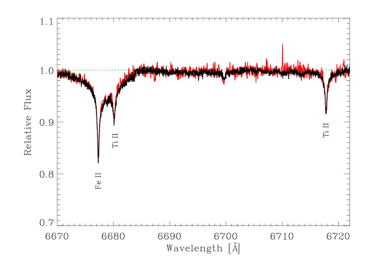
Figure 2: UVES (black) and FEROS (gray/red online) spectra in the region of CL’s Fig. 20. Three absorption features are identified as Fe ii ($\lambda$6677.30), Ti ii ($\lambda$6680.13), and Ti ii ($\lambda$6717.79).

CL discuss three absorption lines in the neighborhood of the broad He i line $\lambda$6678, which they tentatively identify as Fe i $\lambda$6677.989, Ca i $\lambda$6690.628, and Ca i $\lambda$6717.681, with velocity shifts of $-$45, $-$35, and $-$7 $\rm km\,s^{-1}$. Their Fig. 20 shows wavelength shifts at three epochs, best seen in the strongest feature. The upper part of CL’s Fig. 20 closely resembles our spectra, shown in detail in Fig. 2. The broad He i absorption is apparent. We can plausibly identify the sharper absorptions as lines of Fe ii and Ti ii with the radial velocity of the other metallic lines of the shell. Interestingly, $\lambda$6677 of Fe ii does not appear in the current National Institute of Standards and Technology (NIST) list, though it is in the Multiplet Tables, and in the Vienna Atomic Line Database (VALD). G. Nave of NIST (private communication) suggests it is masked in her spectra by an argon line. Our material does not indicate the presence of another star, or another shell with a relative radial velocity shift. We can, of course, not exclude a stage of variability at an epoch not covered by our spectra.

2.2 The metallic lines

Figure 3 is typical of the stronger metallic-line profiles. A rough fit to the observed line is possible with a 10 $\times$ solar abundance and a standard model atmosphere see Sect. 3 for details on the modelling. However, the wings require an impossibly large enhancement of the damping, by 6 $\times$ $10^{3}$. The figure also shows a calculated profile based on a $V\cdot\sin(i)$ of 100 $\rm km\,s^{-1}$and standard Stark broadening.

The stronger metallic-line profiles of HD 94509 gracefully taper to cores as sharp as the instrumental resolution allows. The profiles merge with the continuum in what resemble Lorentz wings. The profiles are very symmetrical, with little or no indication of a wind, or velocity asymmetry within the zone in which they are formed.

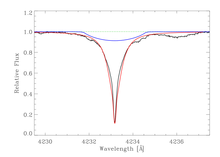
Figure 3: The strong Fe ii line $\lambda$4233, illustrating the unusual metallic-line profiles. The gray (red online) synthesis is based on a $T_{\mathrm{eff}}$ = 10000 K, $\log g$ = 2.5 non-LTE spectrum synthesis model with 10 $\times$ solar abundances, but with the Stark broadening increased by a factor of 6 $\times$ $10^{3}$! The dark gray (blue online) rotational profile used a 10 $\times$ solar iron abundance, with $V\cdot\sin(i)$ = 100 $\rm km\,s^{-1}$ and standard Stark broadening.

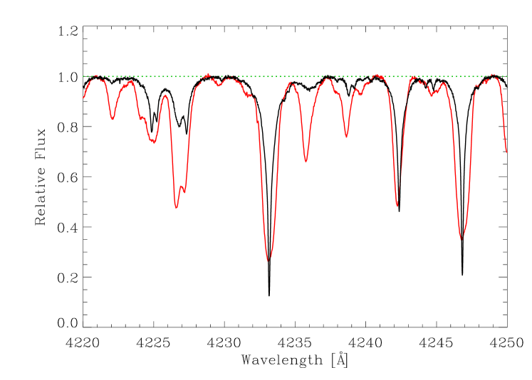
Figure 4: To illustrate the richness of the metallic spectrum of HR 94509, we compare the region of the strong Fe ii line $\lambda$4233, in HD 94509 (black) and that of the F3 Ia supergiant HD 74180 (gray, red online). The somewhat rectangular shape of the profiles with rounded bottoms, of the latter star may be rather closely matched by a model with appropriate microturbulent and rotational broadening.

A broader view of the $\lambda 4233$-region is shown in Fig. 4. The richness of the HD 94509 spectrum is comparable to that of the F3 Ia supergiant HD 74180, and not common among shell stars, cf. Fig. 1. Note we do not imply that HD 94509 is a composite containing such a star. Dilution indicators, discussed below (Section 4.1), show that the metallic-line spectrum of HD 94509 is not photospheric. But a few stable shell stars (Gulliver 1981) may have similar spectra. Merrill (1952) shows a microphotometer tracing for HD 193182, whose spectrum is surely rich in metal lines. We have been unable to find a digital, high-resolution spectrum that would allow us to make a close comparison of the line shapes.

A few of the strong metallic lines show broad emission shoulders as well as relatively narrow, deep absorption. An example is the Fe ii emission, $\lambda$6516: a⁶S_2.5–z⁶D${}^{o}_{3.5}$ in Multiplet 40 (Moore 1945). Multiplet 42 of Fe ii ($\lambda\lambda$4924, 5018, and 5169) is commonly in emission in many peculiar spectra (Be, Herbig Ae/Be, T Tauri). It is is also a sextet to sextet transition involving the same lower (a⁶S) term. Interestingly, Multiplet 42 is at most only weakly in emission in HD 94509.

Figure 5: Base, or full width of 31 Fe ii absorption lines. An average half width for these lines corresponds to a velocity of some 100 $\rm km\,s^{-1}$. No correlation with wavelength is seen. See text for uncertainties in measurements

Figure 6: The base, or full width of Fe ii absorption lines shows a definite correlation with the line depths. For 31 points, the Pearson correlation coefficient is 0.674; the significance, or probability of no correlation is $3\times 10^{-5}$.

In this paper, we will not attempt to account for the overall line shapes, especially the graceful tapering toward the cores of the stronger metallic lines. Figure 3 shows that velocities of the order of 100 $\rm km\,s^{-1}$are required to account for the line wings. If the Doppler effect were responsible for the width of these lines, a correlation of the width with wavelength would be expected. However, such a correlation is not obvious in Fig. 5.

Measurements of the base widths of absorption lines are most uncertain, because a qualitative judgement must be made of the position where the line merges with the continuum. The difficulty is compounded by the presence of blending. Remeasurements of a sample of 10 randomly chosen Fe ii lines shows an average difference of 12%, with an extreme value of 23%. In spite of the uncertainty of these base widths, we do find a significant correlation of the base width with the line depth, as shown in Fig. 6.

We offer no explanation of the unusual line profiles or the correlation of Fig. 6. Widths due to turbulent macroscopic motions would require Mach numbers of 8 or more, and seem unlikely. Rotation of the central star, or Keplerian revolution of a disk could readily produce widths comparable to those measured. It is puzzling that we cannot establish a clear correlation of the line widths with wavelength.

Possibly calculations such as those performed by Hummel & Dachs (1992), but for absorption lines, could account for the line shapes. We must leave this for future work.

2.3 The hydrogen lines

The Balmer lines are highly symmetrical. Both H$\alpha$ and and H$\beta$ have double emission peaks of equal intensity, see Fig. 1. The central absorption cores yield velocities that closely agree with the metallic-line absorption. The central reversals of both H$\alpha$ and H$\beta$ are very deep, while the cores of H$\gamma$, through H$\epsilon$ are virtually black. Our spectra extend from H$\alpha$ to H$\iota$ or H10, and none of the core wavelengths deviate from the laboratory positions by more than 0.04 Å. For such broad profiles, this may easily be attributed to measuring error. The mean deviation for the 9 lower Balmer cores from that expected from the metallic cores is 0.0033 Å. The symmetry of both the hydrogen and metallic absorption cores is indicative of “negligible line-of-sight velocities” in the absorbing shell (cf. Rivinius et al. 2006).

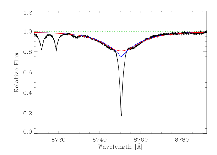
Figure 7: The Paschen line, P12, shows the sharp core of the shell and the broad-line morphology of the central source. Overlaid are rotational profiles for 0 (dark gray, or blue) and 260 $\rm km\,s^{-1}$(light gray, or red). Two N i lines are seen to the violet of P12. See the text for details.

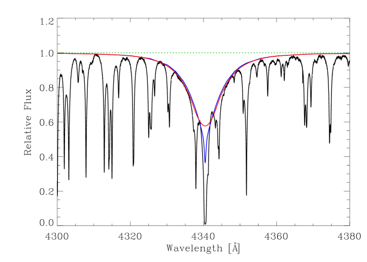
Figure 8: Like Fig. 7, but for H$\gamma$. The black core of the line is indicative for the shell covering the entire stellar disk.

The non-LTE calculations of P12 shown in Fig. 7 were made with a 14000 K, $\log g$ = 3.5 model,assuming an additional continuum equal to a factor of 0.2 times the stellar continuum. Theoretical plots are for $V\cdot\sin(i)$ = 0 and 260 $\rm km\,s^{-1}$. As the Stark-broadened wings of P12 are of stellar origin (only the sharp line core originates in the shell), this may be viewed in support of the atmospheric parameters chosen for the central star (Sect. 6.1). The same applies to other hydrogen lines, also the Balmer lines from H$\gamma$ (see Fig. 8) to the higher series members. A continuum contribution of 0.12 times the central star’s photospheric continuum was adopted for H$\gamma$, meeting the expectation of a decreasing ratio towards the blue. Note, however, that the true amount of dilution of the underlying spectrum is uncertain.

2.4 The helium lines

The He i lines are broad and shallow, unlike the metal lines. They can be matched by rotationally-broadend line profiles, except for cases with metal line blends (see e.g. Fig. 2). This is indication for a stellar atmospheric origin of these lines. They can be fit using atmospheric parameters as adopted for the central star (Sect. 6.1), and a solar helium abundance. Figure 9 shows the example of the line He i $\lambda$5875, assuming an additional continuum from the shell equal to a factor of 0.15 times the stellar continuum, intermediate between the two values adopted for the hydrogen Balmer and Paschen line above. A rotational velocity of $\sim$260 $\rm km\,s^{-1}$ is indicated, in consistency with the typical picture of shell star, where the metallic absorption is superimposed on the spectrum of a rapidly rotating central star.

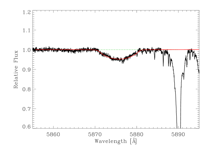
Figure 9: The He i $\lambda$5875 line, which originates in the atmosphere of the central star, with no contribution from the shell. A rotational profile for 260 $\rm km\,s^{-1}$ (light gray, or red) fits the observation. See the text for details.

Table 1: Apparent rotational velocities (half widths) in $\rm km\,s^{-1}$. Emission lines marked with an asterisk. An average is given for the Ca ii infrared triplet.

Spectrum	Wavelength (Å)	$V\cdot\sin(i)$
He i	5876	255
He i	6678	299
Si ii	6347, 6371	245
Ca ii (IRT)∗	8500-8660	225
Ave. 31 Fe ii	3783-7516	99$\pm 33$sd
Fe ii∗	6516	214
K i	7699	114

2.5 Additional remarks

Estimates of the putative $V\cdot\sin(i)$ may be made from the (half) base widths of both additional emission and absorption lines. Uncertainties in these values depend on the line width measurements, whose accuracies are discussed in Section 2.2.

While the metallic spectrum is predominantly absorption, a few lines show “emission shoulders”. Table 1 summarizes the measurements, yielding the following picture. The lines originating from the highest excitation potentials (i.e. the He i lines) indicate the highest apparent rotational velocities, of about 250–300 $\rm km\,s^{-1}$. This should correspond to the rotational velocity of the central star, which is in line with a typical $V\cdot\sin(i)$ that ranges from 200 to 450 $\rm km\,s^{-1}$ for the central component of shell stars (Rivinius et al. 2006). Slightly lower velocities are obtained from the emission shoulders of spectral lines, which arise from the faster-spinning inner parts of the disk. Then, even lower rotational velocities are found for the metallic absorption lines, which involve low-excitation levels and indicate the formation in the slower-rotating outer parts of the disk.

Finally, we note that several broad and shallow features are seen in the spectrum. These coincide in wavelength with several of the typically most pronounced diffuse interstellar bands (DIBs). In particular $\lambda\lambda$5780.45, 6283.86 and 6613.62 are present, but shifted by $\sim+$17 $\rm km\,s^{-1}$ relative to the intrinsic spectrum of HD 94509. This is is consistent with the findings from the sodium D and calcium H and K lines (see Sect. 5).

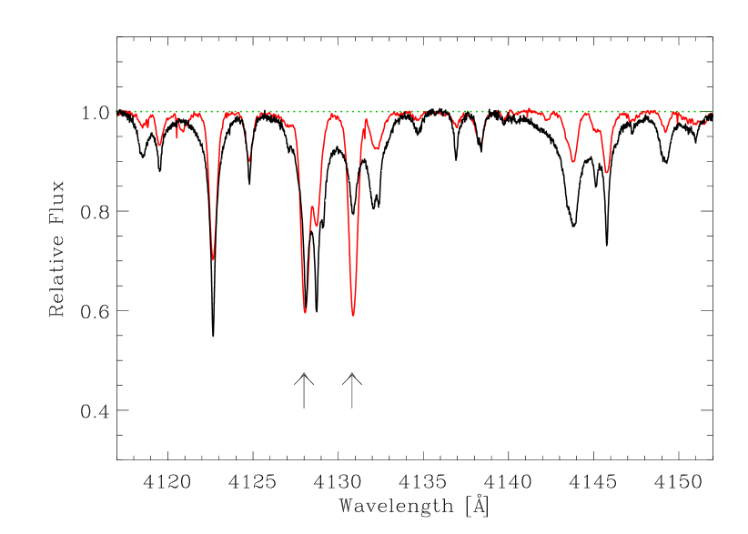
Figure 10: Dilution in the shell of HD 94509. The Si ii lines $\lambda\lambda$4128 and 4130 (arrows) are stronger in the A2 Iae star Deneb (grey, red online) than in HD 94509 (black) because of dilution. The absorption at $\lambda$4128.12 in HD 94509 is largely due to $\lambda$4128.13 of Mn ii.

3 Characterization of the central star

While the overall spectrum is dominated by shell absorption and emission, a small number of features are of photospheric origin, as indicated in the last section: the wings of several hydrogen lines and He i lines. Photospheric metal lines unaffected by disk absorption cannot be identified unambiguously. These lines do not provide sufficient information for a fully-fledged quantitative analysis, but allow an estimate of the atmospheric parameters. A $T_{\mathrm{eff}}$ = 14 000 K and $\log g$ = 3.5, solar helium abundance and $V\cdot\sin(i)$ $\approx$ 260 $\rm km\,s^{-1}$ seems a proper choice, but cannot be considered precise. The presence of He i lines set a lower boundary of the temperature to $\sim$11 000 K. However, this would require an enhanced helium abundance, which is unlikely in view of evolution models for rotating stars that do not predict a noticeable increase of the surface helium values even at critical rotation in the relevant mass range (Brott et al. 2011; Georgy et al. 2013). The wings of the hydrogen lines provide additional information on the effective temperature, but are subject to temperature-gravity degeneracy. Calculations with the ionization code CLOUDY (see Section 6) show that the H$\alpha$ emission strength would be too large for a higher temperature than the one adopted.

The adopted gravity value implies that the star is in an advanced stage of the main-sequence evolution, consistent with theoretical considerations (e.g. Granada et al. 2013). Note that the light from the central star – as a consequence of the fast rotation and the shadowing by the disk seen equator-on (i.e. $i$ $\sim$ 90^o) – is dominated by the hotter and slower-rotating polar caps. Consequently, our above-mentioned parameters are likely upper values for the non-uniform $T_{\mathrm{eff}}$- and $\log g$- distribution over the rotationally-flattened stellar surface, while the rotational velocity is a lower limit (e.g. Townsend et al. 2004; Fremat et al. 2005). The metallicity of the star seems close to solar, or compatible with the present-day cosmic abundance standard (Nieva & Przybilla 2012), as indicated by the analysis of the shell (see Sect. 6).

We employed a hybrid non-LTE approach for our stellar photospheric line-formation calculations, which has been successfully used before in a similar temperature regime to the one studied here (Przybilla et al. 2006; Nieva & Przybilla 2007). Plane-parallel, hydrostatic and homogeneous LTE model atmospheres were computed with the code Atlas9 (Kurucz 1991). Then, non-LTE line-formation computations were performed with the codes Detail and Surface (Giddings 1981; Butler & Giddings 1985, both updated and improved). Detail calculates atomic-level populations by solving the coupled radiative transfer and statistical equilibrium equations, and Surface computes the formal solution using realistic line-broadening functions. We employed model atoms of Przybilla & Butler (2004) for hydrogen, of Przybilla (2005) for He, and of Becker (1998) for Fe ii.

We note that the model calculations are intended to illustrate the plausibility of our parameter choices, but are well aware that this approach is suited to address the complex phenomenology of a Be (shell) star only coarsly. We also note that similar approaches are nevertheless employed for quantitative Be star analyses (e.g. Levenhagen & Leister 2004; Dunstall et al. 2011).

4 Physical conditions in the shell

4.1 Dilution indicators

A general characteristic of shell stars is the relative enhancement of second spectra (from ions) relative to first (from neutrals), when compared with the spectra of dwarfs or normal giants. This may be attributed to the low electron pressure in the shell, which will be discussed in more detail below (cf. Sect. 4.2). A second characteristic, discussed in numerous papers and reviews by Struve (e.g. Struve 1951), is the weakness of certain lines which he called “dilution indicators”. Specifically, Struve called attention to lines of Si ii $\lambda\lambda$3853-3862, 4128-4130, and Mg ii 4481. He noted that the lower levels of the dilution indicators were connected to the ground level by strong permitted transitions. Most absorption lines of Fe ii and Ti ii arise from levels of the same parity as the ground term, and are thus metastable.

We illustrate this in Fig. 10, where lines in HD 94509 and the supergiant Deneb are shown. The latter spectrum is the one described by Schiller & Przybilla (2008). Generally, the metallic lines in HD 94509 are significantly stronger than in Deneb, but this is not the case for Struve’s dilution indicators.

4.2 Electron density

A depth-dependent model of the shell of HD 94509 is beyond the scope of the present work. We attempt to determine mean conditions for the shell as a whole, making use of techniques common for normal stellar atmospheres prior to the use of numerical modeling.

Table 2: Electron densities $\log(N_{e})$

constant	$n=41$	$n=42$
23.26	11.16	11.08
23.49	11.40	11.32

Our high-resolution spectra do not include the Balmer limit, but the Paschen limit is clearly seen. The line P41 was measured, but P42 was not, and an inspection of the spectrum reveals no obvious feature between P41 and three moderate N i lines. A well-established interpretation of the termination of a one-electron line series is that overlapping Stark wings merge so individual features are no longer seen (Inglis & Teller 1939, henceforth, IT). A simple derivation of the formula may be found in Cowley (1970), where it is assumed that protons and electrons contribute equally to the line merging, unlike IT. If the last Paschen line is P$n$, then

$$\log(N_{e})=\log(N_{p})=23.26-7.5\log(n)\,,$$ (1)

where $N_{e}$ and $N_{p}$ are the electron and proton number densities, respectively. Varshni (1978) uses the constant 23.49 rather than 23.26. Let us put $n=41$ and 42 into Eq. 1. Results are shown in Table 2. We conclude that a mean logarithmic electron density of the shell is 11.2$\pm$0.5.

4.3 The shell temperature

4.3.1 Fe ii

We know from the dilution indicators that there can be no single temperature that will describe the excitation and ionization within the shell. Nevertheless, the ionization and excitation may be approximately estimated from measurements of the line strengths. These estimates will be subject to clarification by models of the shell. We have worked primarily with the second spectra of metallic lines: Sc ii, Ti ii, Cr ii, Fe i, Fe ii, and Ni ii. The Fe ii spectrum is by far best suited for our purposes, both because of its richness and the detail of its treatment by the versatile program Cloudy (c13.03, Ferland et al. 2013, cf. Sect. 6.1).

The unusual shape of the Fe ii (and other metallic line) profiles means that measurements of equivalent widths $W_{\lambda}$ require special care. Our general approach in abundance work is to fit metal lines with Voigt profiles. However, the $a=\gamma/(2\Delta\lambda_{D})$ is usually small, typically 0.01 to 0.1, so the profiles are not far from Gaussian. Such a low $a$-value is completely unsuitable for HD 94509. For the lines with profiles that are not too deep, we could make tolerable fits using $a\,=\,5$, virtually Lorentzian profiles. Core and wings of the stronger (deeper) lines could not be fit by any Voigt profile. All of the profiles were also fit with small line segments, so for many lines we could compare the results (Fig. 11). We adopted simple means for all pairs of measurements.

Figure 11: Comparison of $W_{\lambda}$’s (mÅ) measured using segmented profile fits and those using fits to a Voigt profile. the average absolute value of the differences in the plotted equivalent widths is 14 mÅ

One may estimate an overall excitation temperature by plotting $\log(W_{\lambda}/\lambda)$ vs. $\log(gf\lambda)-(5040/T)\cdot\chi$, where $\chi$ is the lower excitation potential of the absorption line. One adopts the temperature $T$ as the value that gives the minimum separation of lines with different $\chi$. We illustrate this determination using reliable Fe ii $gf$-values, from Meléndez & Barbuy (2009, cf. also Adelman 2014). Figure 12 shows the adopted fit, using $\theta\,=\,5040/T\,=\,0.55$, or $T_{\rm exe}\,=\,9164\pm 170$ K. The uncertainty is derived from trial plots with $\theta=0.55$ and 0.56, which were judged marginally acceptable.

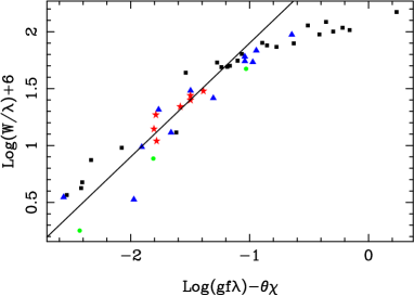
Figure 12: Excitation temperature from Fe ii lines in the shell. Colors may be seen online. The (red) stars indicate lines with the highest lower excitation energies (6.2 to 7.3 eV). The lowest-excitation lines (2.6-2.9 eV) are indicated by black squares. The black line indicates a 45^∘ slope. This plot was made with $\theta\,=\,0.55$ or $T$ = 9164 K with an uncertainty of $\sim$170 K (see text).

4.3.2 Fe i and Ti ii

Other atomic species with enough measurable (mostly unblended) lines to allow a credible curve of growth are Fe i and Ti ii. Results are gathered in Table 3; uncertainty estimates, explained in 4.3.1, are significantly larger for Ti ii and Fe i, which have fewer lines than Fe ii.

Table 3: Excitation temperatures. See text for uncertainty estimates.

Spectrum	No. lines	$\chi$ (eV) range	$T_{\rm ex}$ (K)	Uncertainty (K)
Ti ii	26	0.62 - 3.12	9600	600
Fe i	29	0.00 - 3.63	7750	650
Fe ii	46	2.58 - 7.27	9164	170

4.4 Column densities

The column density of an absorber follows from the relation for weak lines with equivalent widths $W^{\prime}$:

$$W^{\prime}=\frac{\pi e^{2}}{mc^{2}}\lambda^{2}N_{n}f_{nm}.$$ (2)

Here, $N_{n}$ is the number (per cm^-2, column density) in the lower energy level, in the absorbing shell. We have assumed the metal line absorption arises entirely in the shell. In this context we note that the central star has a spectral type in the late/mid-B range and it is unlikely to find chemical peculiarities, as the fast rotation inhibits the CP phenomenon because of rotationally-driven hydrodynamical mixing. Therefore, one may expect the only features of iron-group species present in the stellar spectrum to be weak Fe ii lines. At most, these stellar lines contribute a few percent to the measured equivalent widths, i.e. they are indeed negligible. In fact the presence of strong unusually-shaped features of e.g. Sc ii, Ti ii, Cr ii, Fe i and Ni ii makes the spectrum appear so unusual.

4.4.1 Fe ii

One may estimate from Fig. 12 that lines as strong as 250 mÅ ($\log(W_{\lambda}/\lambda$ + 6 = 1.7, for 5000 Å) are still on the linear part of the curve of growth. Let us make the provisional assumption that iron is predominantly first ionized, neglecting Fe i and Fe iii.

Using the Boltzmann formula, with $u(T)$ the partition function of Fe⁺, and using logarithms, this may be written to give the column density of all Fe⁺ for each line. With $\theta\equiv 5040/T$, and the lower excitation energy $\chi_{n}$, we have

$$\log[N(\mathrm{Fe^{+}})]=\log(W^{\prime}_{\lambda})/\lambda)+12.053-\log(gf\lambda)+\log(u(T))+\theta\chi_{n}.$$ (3)

We work out the column densities for Fe⁺ using Eq. 3 for the Fe ii lines shown in Tab. 4. The average value (of the logarithms) of the last column is 18.77$\pm$0.19.

Table 4: Calculation of column densities for Fe⁺, Dimensions are given for the arguments of the logarithmic quantities.

$\lambda$	$\chi$	$\log(gf)$	$\log[W_{\lambda}]$	$\log[N(\mathrm{Fe}^{+}$)]
Å	eV	no units	mÅ	cm-2
4147.27	4.616	$-$3.508	0.88	18.54
4413.60	2.676	$-$3.79	1.76	18.58
4601.40	2.891	$-$4.48	1.34	18.93
4648.94	2.583	$-$4.58	1.54	19.05
4720.15	3.197	$-$4.48	1.22	18.96
4833.20	2.657	$-$4.64	1.31	18.89
4840.00	2.676	$-$4.75	1.25	18.95
4893.82	2.828	$-$4.21	1.67	18.90
5813.67	5.571	$-$2.51	1.65	18.54
6084.11	3.199	$-$3.79	2.10	18.93
6103.51	6.217	$-$2.171	1.93	18.80
6317.40	6.223	$-$2.16	1.84	18.67
6627.22	7.274	$-$1.609	2.09	18.91
7301.57	3.892	$-$3.63	1.85	18.74
7515.81	3.903	$-$3.39	1.99	18.62
7841.40	3.903	$-$3.721	1.42	18.35
average				18.77$\pm$0.19 (sd)

4.4.2 Neutral iron

While the Fe i lines are less numerous than those of Fe ii, a number of them may be measured, and analyzed in a similar manner. Oscillator strengths for Fe i are from Fuhr & Wiese (2006). Table 5 presents the results. The average of the logarithms for the last column is 15.41$\pm$0.35.

Table 5: Calculation of column densities for neutral Fe or Fe⁰. The format is the same as for Table 4.

$\lambda$	$\chi$	$\log(gf)$	$\log[W_{\lambda}]$	$\log[N(\mathrm{Fe}^{0}$)]
Å	eV	no units	mÅ	cm-2
3873.76	2.43	$-$0.88	1.72	15.52
3983.96	2.73	$-$1.02	1.45	15.54
4118.55	3.63	0.22	1.88	15.20
4134.68	2.83	$-$0.68	1.53	15.30
4175.64	2.84	$-$0.83	1.32	15.24
4181.76	2.83	0.37	1.75	14.46
4309.37	2.95	$-$1.19	1.83	16.15
4442.34	2.20	$-$1.26	1.18	15.11
4459.12	2.18	$-$1.28	1.48	15.42
4466.55	2.83	$-$0.60	1.69	15.32
4476.02	2.84	$-$0.82	1.52	15.37
4494.56	2.20	$-$1.14	1.62	15.43
8688.63	2.18	$-$1.21	1.96	15.26
average				15.33$\pm$0.35 (sd)

4.4.3 Sc ii, Ti ii, Cr ii, and Ni ii

Column densities have been estimated for other species, using the Fe ii curve of growth to choose “weak”’ lines or estimate saturation corrections. Results are discussed in Sect. 6 below. These are uncertain by at least a factor of three because of the difficulty in estimating the contributions from the wings, especially in the case where wings from different lines overlap. Non-LTE effects are also expected, as can be seen from the more detailed results for Fe ii available from Cloudy (cf. Sect. 6).

A resume of observed and theoretical column densities may be found in Sect. 6. Relevant data are presented in Table 9 in Appendix A.

4.4.4 Hydrogen

The highest Paschen lines (those that have no contribution from the central star) may be used to make a crude estimate of the column density $N_{3}$, of hydrogen in the $n=3$ level. Measurements of equivalent widths were made using the segmented fits described above. With Eq. 2, we obtain values of $N_{3}$ that would apply as if the lines were unsaturated. In the ideal case, discussed in the classical text of Unsöld (1955), we would expect values of $N_{3}$ to increase, as the lines become optically thin, and then to decrease as the lines blend together, so their entire width is not measured. Results are shown in Table 6. The line P35 was blended and hence not used. Absorption oscillator strengths were calculated using exact expressions for the wave functions and relevant integrals.

Table 6: Calculation of column densities $N_{3}$ (cm^-2)  for $n=3$, from Paschen lines, P$n$, where $n$ is in the first column.

$n$	$W_{\lambda}$(mÅ)	$f$	$\log(N_{3})$
30	368.	2.034E-04	15.474
31	354.	1.840E-04	15.501
32	259.	1.670E-04	15.408
33	210.	1.521E-04	15.358
34	186.	1.388E-04	15.345
35		1.271E-04
36	160.	1.167E-04	15.355
37	138.	1.075E-04	15.327
38	116.	9.901E-05	15.288
39	90.	9.150E-05	15.212
40	89.	8.474E-05	15.241
41	73.	7.863E-05	15.188
42	61.	7.309E-05	15.138
average			15.32$\pm$0.11 (sd)

The last column of Table 6 decreases as $n$ increases, as expected. We do not see a decrease due to saturation for the smaller $n$. However, the variation from P30 to the last visible line, P42, is not large, so the uncertainty is comparable to other approximations made herein. We adopt $\log(N_{3})\,=\,15.3$.

5 Qualitative chemistry of the circumstellar envelope or shell

Of the lighter elements, hydrogen is well represented by the features described previously. We see broad absorption from He i $\lambda$5876 and 6678, and most of the bluer optical lines, but this is from the underlying stellar spectrum. There is no sign of emission in the He i features. There is also not a hint of absorption or emission at the position of the Li i resonance lines near $\lambda$6708 – which is expected because any lithium initially present would be transported to deeper layers of the stellar envelope due to rotationally-induced mixing, and destroyed by nuclear reactions. This applies in a similar manner to beryllium and boron (relevant lines are located outside the available spectra). Absorption near $\lambda\lambda$9062 and 9112 could be due to C i in Multiplet 3. No C ii lines were noted. A number of absorptions due to N i were identified in the near infrared. Several of these appear in Figs. 1 and 7. The sharp cores of the N i lines are indicative of absorption from the shell. Neutral oxygen lines from the shell are the strong infrared triplet $\lambda\lambda$7772, 7774, and 7775 and the line $\lambda$8446 (see Fig. 1).

The D lines of sodium are strong. Each line is double, with the deeper component having the stellar radial velocity, with the strong, second component shifted to the red by 17.3 $\rm km\,s^{-1}$, likely being of interstellar origin (an analogous situation is seen in the calcium H and K lines). Several lines of Mg i are identified including the b-lines, which have the broad wings and sharp cores of the shell. The usually strong Mg ii $\lambda$4481 is severely weakened as noted earlier. The Al i resonance doublet is present, but weak. No Si i lines were identified, but Si ii lines are present in addition to the dilution indicators mentioned in Sect. 4.1. The violet component of the K i resonance pair, $\lambda$7665 is obscured by water-vapor absorption, but $\lambda$7699 is unblended and strong ($W_{\lambda}$ $\approx$ 500 mÅ), see Fig. 1. The 3$d$ elements Ca-Ni are all well represented, but heavier elements are weak or absent altogether, similar to the situation in a supergiant spectrum at comparable temperature.

An analysis by wavelength coincidence statistics (WCS) reveals meager evidence for the presence of neutron addition elements. Even the Sr ii resonance lines, $\lambda\lambda$4077 and 4215 are weak and blended. Neither of the Ba ii resonance lines, $\lambda\lambda$4554 and 4934 show more than a possibility of absorption near their positions. This need not imply an underabundance of Ba or Sr as we anticipate significant double ionization of these two elements. Zr ii may be weakly present, but there is no evidence for Y ii.

Table 7: Characteristics of the Cloudy model which fit the observations as summarized in Table 8. Keplerian velocities, $V_{K}$ are in $\rm km\,s^{-1}$, for a 4.2 $M_{\odot}$ star.

Central star	$T_{\rm eff}=14000$K, $\log g=3.5$
Stellar luminosity	$2.4\times 10^{36}$ erg s-1
Stellar radius	4.2 $R_{\odot}$
Inner cloud radius	14.4 $R_{\odot}$; $V_{K}=236$ $\rm km\,s^{-1}$
Outer cloud radius	45.5 $R_{\odot}$; $V_{K}=133$ $\rm km\,s^{-1}$
Cylinder semi-height	5.0 $R_{\odot}$
Total hydrogen density	$1.58\cdot 10^{11}$ cm-3 (constant)
Average electron density	$9.8\cdot 10^{10}$ cm-3 (variable)
Molecules and grains	off

6 A model using Cloudy

6.1 Details

It is clear that the conditions in the shell cannot be well described by local thermodynamic equilibrium (LTE). We have therefore used the versatile photoionization code Cloudy (Ferland et al. 2013) to broaden our analysis. Ideally, we would run cloudy as a subroutine, and try to minimize deviations of its predictions against our measurements. Such an approach is beyond the scope of the present work. We have limited ourselves to trial and error comparisons of selected measurements or derived quantities, assuming default solar abundances (Asplund et al. 2009; Scott et al. 2015a, b; Grevesse et al. 2015).

The stellar background is from a Kurucz (1991) Atlas9 model. Details, and some relevant quantities are collected in Table 7. Properties for the $T_{\rm eff}$ = 14 000 K main sequence star were chosen with the help of data from Torres et al. (2011). We report results here for a cylindrical geometry described in the documentation for Cloudy (Hazy-1, Sect. 9.6). Similar results were obtained with a spherical geometry with the same parameters apart from the cylinder height.

It is possible to obtain column densities for any one of 371 individual levels of Fe⁺. Our models used 256 levels, to save computing time. We may obtain an “excitation temperature” from these column densities that should be comparable to the values derived by the empirical curves of growth from Ti ii, Fe i, and Fe ii. This is shown in Fig. 13.

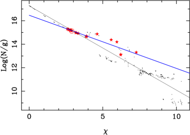
Figure 13: Theoretical “excitation temperatures” from column densities for Fe ii levels of the Cloudy models. The quantity $g$ is the statistical weight, $2J+1$, of the levels. The larger symbols are for levels that correspond to the lines used in Fig. 12. The heavy line is a least squares solution giving $T$ = 11134 K. Smaller symbols are for all 256 levels used in the model; the lighter line corresponds to $T$ = 7026 K.

Recall that the empirical results for Fe ii and Ti ii were $\sim$9164 K, while that for Fe i was 7750 K. Theoretical and empirical results are summarized in Table 8. The “empirical” entries for neutral and ionized hydrogen are described as semi-empirical and shown inside brackets. While the IT formula allows us to estimate a mean electron density (cm^-3), we can only infer a column density indirectly. The entry for H⁺ in Table 8 comes from taking the product of the IT electron density and multiplying by the physical thickness of the model, to obtain a column density. We assume the column density of protons is reasonably approximated by the electron column density thus obtained.

We have an empirical estimate of the column density only for the $n\,=\,3$ level of neutral hydrogen. We need a temperature to convert this to a column density for all levels of hydrogen, using the Boltzmann formula. There is no obvious empirical value to use; indeed, because of the non-LTE conditions the meaning of any temperature so chosen is strictly limited to the Boltzmann formula and the relevant level populations. If we simply define a $T_{\rm ex}$ as that value giving the column densities $N_{3}$(H) and $N$(H), the adopted CLOUDY model gives $5040/T_{\rm ex}$ = 0.69. Recall the empirical values of $\theta$ from Fe i and Fe ii were 0.65 and 0.55. The entry for H⁰ in Table 8 was obtained using $\theta$ = 0.69, and the empirical $\log(N_{3}$(H)) = 15.3.

Let us assume (Hanuschik 1996) that Be and shell stars have “disks that are intrinsically identical.” Then our basic parameters from Table 8 should be comparable with those estimated for Be stars. These stars display a variety of characteristics, summarized by Slettebak and Smith (2000). The stellar types range from late O (X Per) to late B ($\beta$ CMi). The disks are typically 5 to 20 stellar radii, with temperatures of 10 000K, and electron densities of 10¹⁰ to 10¹³ per cm. Our values for $N_{\rm e}$, $T$, and radii agree well with these values.

Table 8: Comparison of various empirical results with corresponding quantities from the model using solar abundances. Numerical values without units are logarithms of column densities (cm^-2). Neutral species are indicated by a superscript ‘$0$’. Parenthesized numbers indicate the number of lines used. Values in square brackets are semi-empirical (see text).

Species	Model	Empirical
H0	23.30	[22.8]
H+	23.15	[23.5]
N3(H)	15.85	15.3
$\log(N_{e})$(cm${}^{-3})$	10.99	11.2
Sc+	14.54	15.2(2)
Ti+	16.43	16.8(5)
Cr+	17.11	17.2(4)
Fe0	14.25	15.4(13)
Fe+	18.98	18.8(16)
Ni+	17.74	17.6(4)
$T_{\rm ex}$ (K)	11134	9164
$W_{\lambda}$(H$\alpha$) (Å)	28	24

6.2 Comments

The dominant species, e.g. Fe⁺ are predicted reasonably well by the model. For column and particle densities in Table 8, apart from neutral iron, the rms deviations of the empirical from the 9 model values is 0.33 dex, or a factor of 2.1. Neutral iron is an order of magnitude or more stronger than the predictions. If we include neutral iron, the rms deviation is 0.42 dex. A cooler central star could reduce this discrepancy, but the broad He i absorptions would then be difficult to explain. It does not help the ionization discrepancy to move the cloud out by a factor of 10. Higher or lower overall densities were also tried, with appropriate adjustments of the absorption path lengths.

We note that the treatment of complex atoms of the iron group by Cloudy, apart from Fe ii, does not involve multi-level models. In view of this approximate treatment, we do not consider the discrepancy with the Fe i column density to be serious in the context of the present study.

7 Conclusions

HD 94509 is a shell star with an unusually stable shell, posing an extreme in the zoo of Be star spectral morphology. We have not been able to account for the unusual shapes of the metallic absorption lines. However a simple model of the shell can predict the total absorption from H i, the electron density, and column densities of the dominant ions. Near-solar elemental abundances are found. The lowest Balmer lines have deep cores and symmetrical emissions. The cores of H$\gamma$ through H$\epsilon$ are virtually black, indicating the shell must cover the stellar disk.

Appendix A Data on iron group elements

Table 9: Data for lines used for column densities of elements other than iron. References are to the oscillator strength source.

Wavelength [Å]	$\chi$ (eV)	$\log(gf)$	$W_{\lambda}$ (mÅ)
Sc ii, Lawler & Dakin (1989)
4246.82	0.315	0.242	616
4400.49	0.605	$-$0.536	304
4415.56	0.595	$-$0.668	491
4420.67	0.618	$-$2.273	20
Ti ii, Pickering et al. (2001, 2002)
4025.13	0.61	$-$2.14	310
4028.34	1.89	$-$0.96	318
4227.35	1.13	$-$2.24	169
4287.87	1.08	$-$1.82	250
4290.22	1.17	$-$0.85	455
4300.05	1.18	$-$0.44	532
4312.86	1.18	$-$1.10	434
4391.03	1.23	$-$2.28	166
4398.29	1.22	$-$2.78	86
4399.77	1.24	$-$1.19	414
4411.93	1.22	$-$2.52	98
4432.11	1.24	$-$2.81	47
4441.73	1.18	$-$2.27	190
4443.79	1.08	$-$0.72	430
4450.48	1.08	$-$1.52	418
4464.45	1.16	1.81	276
4468.51	1.13	$-$0.60	506
4501.27	1.12	$-$0.77	568
4518.33	1.08	$-$2.91	91
Cr ii, Nilsson et al. (2006)
4195.42	5.32	$-$1.95	41
4242.36	3.87	$-$1.17	324
4558.66	4.07	$-$0.656	616
4588.20	4.07	$-$0.627	545
4634.07	4.07	$-$0.980	454
4812.34	3.86	$-$1.800	341
4824.13	3.87	$-$0.920	500
4836.23	3.86	$-$2.25	137
Ni ii, Kurucz (2014)
4015.47	4.03	$-$2.41	58
4067.03	4.03	$-$1.83	269
4244.78	4.03	$-$3.10	17
4362.10	4.03	$-$2.70	59