A Variance Reduced Stochastic Newton Method

Abstract

Quasi-Newton methods are widely used in practise for convex loss minimization problems. These methods exhibit good empirical performance on a wide variety of tasks and enjoy super-linear convergence to the optimal solution. For large-scale learning problems, stochastic Quasi-Newton methods have been recently proposed. However, these typically only achieve sub-linear convergence rates and have not been shown to consistently perform well in practice since noisy Hessian approximations can exacerbate the effect of high-variance stochastic gradient estimates. In this work we propose Vite, a novel stochastic Quasi-Newton algorithm that uses an existing first-order technique to reduce this variance. Without exploiting the specific form of the approximate Hessian, we show that Vite reaches the optimum at a geometric rate with a constant step-size when dealing with smooth strongly convex functions. Empirically, we demonstrate improvements over existing stochastic Quasi-Newton and variance reduced stochastic gradient methods.

1 Introduction

We consider the problem of optimizing a function expressed as an expectation over a set of data-dependent functions. Stochastic gradient descent (SGD) has become the method of choice for such tasks as it only requires computing stochastic gradients over a small subset of datapoints [2, 18]. The simplicity of SGD is both its greatest strength and weakness. Due to the effects of evaluating noisy approximation of the true gradient, SGD achieves a convergence rate which is only sub-linear in the number of steps. In an effort to deal with this randomness, two primary directions of focus have been developed. The first line of work focuses on choosing the appropriate SGD step-size [1, 10, 14]. If a decaying step-size is chosen, the variance is forced to zero asymptotically guaranteeing convergence. However, small steps also slow down progress and limit the rate of convergence in practise. The step-size must be chosen carefully, which can require extensive experimentation possibly negating the computational speedup of SGD. Another approach is to use an improved, lower-variance estimate of the gradient. If this estimator is chosen correctly – such that its variance goes to zero asymptotically – convergence can be guaranteed with a constant learning rate. This scheme is used in [5, 16] where the improved estimate of the gradient combines stochastic gradients computed at the current stage with others used at an earlier stage. A similar approach proposed in [8, 9] combines stochastic gradients with gradients periodically re-computed at a pivot point.

With variance reduction, first-order methods can obtain a linear convergence rate. In contrast, second-order methods have been shown to obtain super-linear convergence. However, this requires the computation and inversion of the Hessian matrix which is impractical for large-scale datasets. Approximate variants known as quasi-Newton methods [6] have thus been developed, such as the popular BFGS or its limited memory version known as LBFGS [11]. Quasi-Newton methods such as BFGS do not require computing the Hessian matrix but instead construct a quadratic model of the objective function by successive measurements of the gradient. This also yields super-linear convergence when the quadratic model is accurate. Stochastic variants of BFGS have been proposed (oBFGS [17]), for which stochastic gradients replace their deterministic counterparts. A regularized version known as RES [12] achieves a sublinear convergence rate with a decreasing step-size by enforcing a bound on the eigenvalues of the approximate Hessian matrix. SQN [3], another related method also requires a decreasing step size to achieve sub-linear convergence. Although stochastic second order methods have not be shown to achieve super-linear convergence, they empirically outperform SGD for problems with a large condition number [12].

A clear drawback to stochastic second order methods is that similarly to their first-order counterparts, they suffer from high variance in the approximation of the gradient. Additionally, this problem can be exaggerated due to the estimate of the Hessian magnifying the effect of this noise. Overall, this can lead to such algorithms taking large steps in poor descent directions.

In this paper, we propose and analyze a stochastic variant of BFGS that uses a multi-stage scheme similar to [8, 9] to progressively reduce the variance of the stochastic gradients. We call this method Variance-reduced Stochastic Newton (Vite). Under standard conditions on $\hat{J}$, we show that that variance reduction on the gradient estimate alone is sufficient for fast convergence. For smooth and strongly convex functions, Vite reaches the optimum at a geometric rate with a constant step-size. To our knowledge Vite is the first stochastic Quasi-Newton method with these properties.

In the following section, we briefly review the BFGS algorithm and its stochastic variants. We then introduce the VITE algorithm and analyze its convergence properties. Finally, we present experimental results on real-world datasets demonstrating its superior performance over a range of competitors.

2 Stochastic second order optimization

2.1 Problem setting

Given a dataset ${\mathcal{D}}=\{({\bf x}_{1},y_{1}),\dots,({\bf x}_{n},y_{n})\}$ consisting of feature vectors ${\bf x}_{i}\in\mathbb{R}^{d}$ and targets $y_{i}\in[0,C]$, we consider the problem of minimizing the expected loss $f({\bf w})={\mathbb{E}}[f_{i}({\bf w})]$. Each function $f_{i}({\bf w})$ takes the form $f_{i}({\bf w})=\ell(h({\bf w},{\bf x}_{i}),y_{i}),$ where $\ell$ is a loss function and $h$ is a prediction model parametrized by ${\bf w}\in\mathbb{R}^{d}$. The expectation is over the set of samples and we denote ${\bf w}^{*}=\arg\min_{{\bf w}}f({\bf w})$.

This optimization problem can be solved exactly for convex functions using gradient descent, where the gradient of the loss function is expressed as $\nabla_{{\bf w}}f({\bf w})={\mathbb{E}}[\nabla_{{\bf w}}f_{i}({\bf w})]$. When the size of the dataset $n$ is large, the computation of the gradient is impractical and one has to resort to stochastic gradients. Similar to gradient descent, stochastic gradient descent updates the parameter vector ${\bf w}_{t}$ by stepping in the opposite direction of the stochastic gradient $\nabla_{{\bf w}}f_{i}({\bf w}_{t})$ by an amount specified by a step size $\eta_{t}$ as follows:

$${\bf w}_{t+1}={\bf w}_{t}-\eta_{t}\nabla_{{\bf w}}f_{i}({\bf w}_{t}).$$ (1)

In general, a stochastic gradient can also be computed as an average over a sample of datapoints as $\hat{f}({\bf w}_{t})=r^{-1}\sum_{i=1}^{r}f_{i}({\bf w}_{t})$. Given that the stochastic gradients are unbiased estimates of the gradient, Robbins and Monro [15] proved convergence of SGD to ${\bf w}^{*}$ assuming a decreasing step-size sequence. A common choice for the step size is [18, 12]

$$\it{a)}\;\eta_{t}=\frac{\eta_{0}}{t}\quad\quad\text{or}\quad\quad\it{b)}\;\eta_{t}=\frac{\eta_{0}T_{0}}{T_{0}+t}$$ (2)

where $\eta_{0}$ is a constant initial step size and $T_{0}$ controls the speed of decrease.

Although the cost per iteration of SGD is low, it suffers from slow convergence for certain ill-conditioned problems [12]. An alternative is to use a second order method such as Newton’s method that estimates the curvature of the objective function and can achieve quadratic convergence. In the following, we review Newton’s method and its approximations known as quasi-Newton methods.

2.2 Newton’s method and BFGS

Newton’s method is an iterative method that minimizes the Taylor expansion of $f({\bf w})$ around ${\bf w}_{t}$:

$$f({\bf w})= f({\bf w}_{t})+({\bf w}-{\bf w}_{t})^{\top}\nabla_{{\bf w}}f({\bf w}_{t})+\frac{1}{2}({\bf w}-{\bf w}_{t})^{\top}H({\bf w}-{\bf w}_{t}),$$ (3)

where $H$ is the Hessian of the function $f({\bf w})$ and quantifies its curvature. Minimizing Eq. 3 leads to the following update rule:

$${\bf w}_{t+1}={\bf w}_{t}-\eta_{t}H_{t}^{-1}\cdot\nabla f({\bf w}_{t}),$$ (4)

where $\eta_{t}$ is the step size chosen by backtracking line search.

Given that computing and inverting the Hessian matrix is an expensive operation, approximate variants of Newton’s method have emerged, where $H_{t}^{-1}$ is replaced by an approximate version $\tilde{H}_{t}^{-1}$ selected to be positive definite and as close to $H_{t}^{-1}$ as possible. The most popular member of this class of quasi-Newton methods is BFGS [13] that incrementally updates an estimate of the inverse Hessian, denoted $J_{t}=\tilde{H}_{t}^{-1}$. This estimate is computed by solving a weighted Frobenius norm minimization subject to the secant condition:

$${\bf w}_{t+1}-{\bf w}_{t}=J_{t+1}(\nabla f({\bf w}_{t+1})-\nabla f({\bf w}_{t})).$$ (5)

The solution can be obtained in closed form leading to the following explicit expression:

$$J_{t+1}=\left(I-\frac{sy^{\top}}{y^{\top}s}\right)J_{t}\left(I-\frac{ys^{\top}}{y^{\top}s}\right)+\frac{ss^{\top}}{y^{\top}s},$$ (6)

where $s={\bf w}_{t+1}-{\bf w}_{t}$ and $y=\nabla f({\bf w}_{t+1})-\nabla f({\bf w}_{t})$. Eq. 6 is known to be positive definitive assuming that $J_{0}$ is initialized to be a positive definite matrix.

2.3 Stochastic BFGS

A stochastic version of BFGS (oBFGS) was proposed in [17] in which stochastic gradients are used for both the determination of the descent direction and the approximation of the inverse Hessian. The oBFGS approach described in Algorithm 1 uses the following update equation:

$${\bf w}_{t+1}={\bf w}_{t}-\eta_{t}\hat{J}_{t}\cdot\nabla\hat{f}({\bf w}_{t}),$$ (7)

where the matrix $\hat{J}_{t}$ and the vector $\nabla\hat{f}({\bf w}_{t})$ are stochastic estimates computed as follows. Let ${\mathcal{A}}\subset\{1\dots n\}$ and ${\mathcal{B}}\subset\{1\dots n\}$ be sets containing two independent samples of datapoints. The variables $y$ and $\nabla f({\bf w})$ defined in Eq. 6 are replaced by sampled variables computed as

$$\hat{y}=\frac{1}{|{\mathcal{A}}|}\sum_{k\in{\mathcal{A}}}\nabla f_{k}({\bf w}_{t+1})-\nabla f_{k}({\bf w}_{t})\quad\text{and}\quad\nabla\hat{f}({\bf w}_{t})=\nabla f_{{\mathcal{B}}}({\bf w}_{t})=\frac{1}{|{\mathcal{B}}|}\sum_{k\in{\mathcal{B}}}\nabla f_{k}({\bf w}_{t}).$$ (8)

The estimate of the inverse Hessian then becomes

$$\hat{J}_{t+1}=\left(I-\frac{s\hat{y}^{\top}}{\hat{y}^{\top}s}\right)\hat{J}_{t}\left(I-\frac{\hat{y}s^{\top}}{\hat{y}^{\top}s}\right)+\frac{ss^{\top}}{\hat{y}^{\top}s}$$ (9)

Unlike Newton’s method, oBFGS uses a fixed step size sequence instead of a line search. A common choice is to use a step size similar to the one used for SGD in Eq. 2.

Algorithm 1 oBFGS

1:  INPUTS :

2:     $\mathcal{D}$ : Training set of $n$ examples.

3:     ${\bf w}_{0}$ : Arbitrary initial values, e.g., 0.

4:     $\{\eta_{t}\}$ : Step size sequence

5:  OUTPUT : ${\bf w}_{t}$

6:  $\hat{J}_{0}\leftarrow\alpha I$

7:  for $t=0\dots T$ do

8:     Randomly pick two sets ${\mathcal{A}}$ and ${\mathcal{B}}$

9:     $s\leftarrow{\bf w}_{t+1}-{\bf w}_{t}$

10:     $\hat{y}\leftarrow\sum_{k\in{\mathcal{B}}}\nabla f_{k}({\bf w}_{t+1})-\nabla f_{k}({\bf w}_{t})$

11:     $\nabla\hat{f}({\bf w}_{t})\leftarrow\sum_{k\in{\mathcal{A}}}\nabla f_{k}({\bf w}_{t})$

12:     ${\bf w}_{t+1}\leftarrow{\bf w}_{t}-\eta_{t}\hat{J}_{t+1}\cdot\nabla\hat{f}({\bf w}_{t})$

13:     $\hat{J}_{t+1}\leftarrow\left(I-\frac{s\hat{y}^{\top}}{\hat{y}^{\top}s}\right)\hat{J}_{t}\left(I-\frac{\hat{y}s^{\top}}{\hat{y}^{\top}s}\right)+\frac{ss^{\top}}{\hat{y}^{\top}s}$

14:  end for

A regularized version of oBFGS (RES) was recently proposed in [12]. RES differs from oBFGS in the use of a regularizer to enforce a bound on the eigenvalues of $\hat{J}_{t}$ such that

$$\gamma I\preceq\hat{J}_{t}\preceq\rho I=\left(\gamma+\frac{1}{\delta}\right)I,$$ (10)

where $\gamma$ and $\delta$ are given positive constants and the notation $A\preceq B$ means that $B-A$ is a positive semi-definite matrix. Note that (10) also implies an upper and lower bound on ${\mathbb{E}}[\hat{J}_{t}]$ [12]. The update of RES is modified to incorporate an identity bias term $\gamma I$ as follows:

$${\bf w}_{t+1}={\bf w}_{t}-\eta_{t}(\hat{J}_{t}+\gamma I)\cdot\nabla\hat{f}({\bf w}_{t}).$$ (11)

The convergence proof derived in [12] shows that lower and upper bounds on the Hessian eigenvalues of the sample functions are sufficient to guarantee convergence to the optimum. However, the analysis shows that RES will converge to the optimum at a rate $\mathcal{O}(1/t)$ and requires a decreasing step-size. Similar results were derived in [3] for the SQN algorithm.

3 The Vite algorithm

Reducing the size of the sets ${\mathcal{A}}$ and ${\mathcal{B}}$ used to estimate the inverse Hessian approximation and the stochastic gradient is desirable for reasons of computational efficiency. However, doing so also increases the variance of the update step. Here we propose a new method called Vite that explicitly reduces this variance.

In order to simplify the analysis of Vite, we do not explicitly consider the randomness in the matrix $\hat{J}_{t}$. Instead, we assume that it is positive definite (which holds under weak conditions due to the BFGS update step) and that its variance can be kept under control, for example by using the regularization of the RES method.

To motivate Vite we first consider the standard oLBFGS step, (7) estimated with the sets ${\mathcal{A}}$ and ${\mathcal{B}}$. The first and second moments simplify as

$${\mathbb{E}}~{}[\hat{J}_{t}\nabla f_{{\mathcal{B}}}({\bf w}_{t})]=\hat{J}_{t}{\mathbb{E}}_{{\mathcal{B}}}[\nabla f_{{\mathcal{B}}}({\bf w}_{t})]$$ (12)

and

$${\mathbb{E}}~{} \left|\left|\hat{J}_{t}\nabla f_{{\mathcal{B}}}({\bf w}_{t})\right|\right|^{2}\leq\left|\left|\hat{J}_{t}\right|\right|^{2}{\mathbb{E}}_{{\mathcal{B}}}\left|\left|\nabla f_{{\mathcal{B}}}({\bf w}_{t})\right|\right|^{2},$$ (13)

respectively. For $|{\mathcal{A}}|$ large enough, in order to reduce the variance of the estimate $\hat{J}_{t}\cdot\nabla f_{{\mathcal{B}}}({\bf w}_{t})$, it is only required to reduce the variance of $\nabla{f}_{{\mathcal{B}}}({\bf w}_{t})$ independently. We proceed using a technique similar to the one proposed in [8, 9].

Vite differs from oBFGS and other stochastic Quasi-Newton methods in the use of a multi-stage scheme as shown in Algorithm 2. In the outer loop a variable ${\tilde{\bf w}}$ is introduced. We periodically evaluate the gradient of the function with respect to ${\tilde{\bf w}}$. This pivot point is inserted in the update equation to reduce the variance. Each inner loop runs for a a random number of steps $t_{j}\in[1,m]$ whose distribution follows a geometric law with parameter $\beta=\sum_{t=1}^{m}(1-\mu\gamma\eta)^{m-t}$. Stochastic gradients at ${\bf w}_{t}$ and ${\tilde{\bf w}}$ are computed and the inverse Hessian approximation is updated in each iteration of the inner loop. $\hat{J}_{t}$ can be updated using the same update as RES although we found in practice that using Eq. 9 did not affect the results significantly. The descent direction $\nabla f_{{\mathcal{B}}}({\bf w})$ is then replaced by

$${\bf v}_{t}=\nabla f_{{\mathcal{B}}}({\bf w}_{t})-\nabla f_{{\mathcal{B}}}({\tilde{\bf w}})+\tilde{\nu}.$$

Vite then makes updates of the form

$${\bf w}_{t+1}={\bf w}_{t}-\eta\hat{J}_{t}\cdot{\bf v}_{t}.$$ (14)

Clearly, $\tilde{\nu}={\mathbb{E}}[\nabla f_{{\mathcal{B}}}({\tilde{\bf w}})]$ and ${\mathbb{E}}[{\bf v}_{t}]={\mathbb{E}}[\nabla f_{{\mathcal{B}}}({\bf w}_{t})]$ so in expectation the descent is in the same direction as Eq. (12). Following the analysis of [8], the variance of ${\bf v}_{t}$ goes to zero when both ${\tilde{\bf w}}$ and ${\bf w}_{t}$ converge to the same parameter ${\bf w}^{*}$. Therefore, convergence can be guaranteed with a constant step-size. The complexity of this approach depends on the number of epochs $S$ and a constant $m$ limiting the number of stochastic gradients computed in a single epoch, as well as other parameters that will be introduced in more detail in Section 4.

Algorithm 2 Vite

1:  INPUTS :

2:     $\mathcal{D}$ : Training set of $n$ examples    ${\tilde{\bf w}}_{0}$ : Arbitrary initial values, e.g., 0

3:     $\eta$ : Constant step size        $m$: Arbitrary constant

4:  OUTPUT : ${\bf w}_{t}$

5:  $\hat{J}_{0}\leftarrow\alpha I$

6:  for $s=0\dots S$ do

7:     ${\tilde{\bf w}}={\tilde{\bf w}}_{s-1}$

8:     $\tilde{\nu}=\frac{1}{n}\sum_{i=1}^{n}\nabla f_{i}({\tilde{\bf w}})$

9:     ${\bf w}_{0}={\tilde{\bf w}}$

10:     Let $t_{j}\leftarrow t$ with probability $\frac{(1-\mu\rho\eta)^{m-t}}{\beta}$ for $t=1,\dots,m$

11:     for $t=0\dots t_{j}-1$ do

12:        Randomly pick independent sets ${\mathcal{A}},{\mathcal{B}}\subset\{1\dots n\}$

13:        ${\bf v}_{t}=\nabla f_{{\mathcal{B}}}({\bf w}_{t})-\nabla f_{{\mathcal{B}}}({\tilde{\bf w}})+\tilde{\nu}$

14:        ${\bf w}_{t+1}\leftarrow{\bf w}_{t}-\eta\hat{J}_{t}\cdot{\bf v}_{t}$

15:        Update $\hat{J}_{t+1}$

16:     end for

17:     ${\tilde{\bf w}}_{s}={\bf w}_{t_{j}}$.

18:  end for

4 Analysis

In this section we present a convergence proof for the Vite algorithm that builds upon and generalizes previous analyses of variance reduced first order methods [8, 9]. Specifically, we show how variance reduction on the stochastic gradient direction is sufficient to establish geometric convergence rates, even when performing linear transformations with a matrix $\hat{J}_{t}$. Since we do not exploit the specific form of the stochastic evolution equations for $\hat{J}_{t}$, this analysis will not allow us to argue in favor of the specific choice of Eq. (9), yet it shows that variance reduction on the gradient estimate is sufficient for fast convergence as long as $\hat{J}_{t}$ is sufficiently well behaved. Our analysis relies on the following standard assumptions:

A1

Each function $f_{i}$ is differentiable and has a Lipschitz continuous gradient with constant $L>0$, i.e. $\forall{\mathbf{w}},{\mathbf{v}}\in\mathbb{R}^{n}$,

$$f_{i}({\mathbf{w}})\leq f_{i}({\mathbf{v}})+({\mathbf{w}}-{\mathbf{v}})^{\top}\nabla f_{i}({\mathbf{v}})+\frac{L}{2}\left|\left|{\mathbf{w}}-{\mathbf{v}}\right|\right|^{2}$$ (15)

A2

$f$ is $\mu$-strongly convex, i.e. $\forall{\mathbf{w}},{\mathbf{v}}\in\mathbb{R}^{n}$,

$$f({\mathbf{w}})\geq f({\mathbf{v}})+({\mathbf{w}}-{\mathbf{v}})^{\top}\nabla f({\mathbf{v}})+\frac{\mu}{2}\left|\left|{\mathbf{w}}-{\mathbf{v}}\right|\right|^{2}$$ (16)

which also implies

$$\left|\left|\nabla f({\bf w})\right|\right|^{2}\geq 2\mu(f({\bf w})-f({\bf w}^{*}))\;\;\forall{\bf w}\in\mathbb{R}^{n}$$ (17)

for the minimizer ${\bf w}^{*}$ of $f$.

Assumptions A1 and A2 also implies that the eigenvalues of the Hessian are bounded as follows:

$$\mu I\preceq H_{t}\preceq LI.$$ (18)

Finally we make the assumption that the inverse Hessian approximation is always well-behaved.

A3

There exist positive constants $\gamma$ and $\rho$ such that, $\forall{\bf w}\in\mathbb{R}^{n}$,

$$\gamma I\preceq\hat{J}_{t}\preceq\rho I.$$ (19)

Assumption A3 is equivalent to assuming that $\hat{J}_{t}$ is bounded in expectation (see: e.g. [12]) but allows us to remove this complication, simplifying notation in the analysis which follows. We now introduce two lemmas required for the proof of convergence.

Lemma 1.

The following identity holds:

$${\mathbb{E}}f({\tilde{\bf w}}_{s+1})=\frac{1}{\beta}\sum_{t=0}^{m-1}\tau_{t}{\mathbb{E}}f({\bf w}_{t})$$

where $\tau_{t}:=(1-\gamma\eta\mu)^{m-t-1}$ and the weight vectors ${\bf w}_{t}$ belong to epoch $s$.

This result follows directly from Lemma 3 in  [9].

Lemma 2.

$${\mathbb{E}}\|{\bf v}_{t}\|^{2} \leq 4L(f({\bf w}_{t})-f({\bf w}^{*})+f({\tilde{\bf w}})-f({\bf w}^{*}))$$

The proof is given in [8, 9] and reproduced for convenience in the Appendix. We are now ready to state our main result.

Theorem 1.

Let Assumptions A1-A3 be satisfied. Define the rescaled strong convexity $\mu^{\prime}:=\gamma\mu\leq\mu$ and Lipschitz $L^{\prime}:=\rho L\geq L$ constants respectively. Choose $0<\eta\leq\frac{\mu^{\prime}}{2{L^{\prime}}^{2}}$ and let m be sufficiently large so that $\alpha=\frac{(1-\eta\mu^{\prime})^{m}}{\beta\eta(\mu^{\prime}-2{L^{\prime}}^{2}\eta)}+\frac{2{L^{\prime}}^{2}\eta}{\mu^{\prime}-2{L^{\prime}}^{2}\eta}<1.$

Then the suboptimality of ${\tilde{\bf w}}_{s}$ is bounded in expectation as follows:

$${\mathbb{E}}(f({\tilde{\bf w}}_{s})-f({\bf w}^{*}) \leq\alpha^{s}{\mathbb{E}}[f({\bf w}_{0})-f({\bf w}^{*})].$$ (20)

Remark 1.

Observe that $\gamma$ and $\rho$ are bounds on the inverse Hessian approximation. If $\hat{J}_{t}$ is a good approximation to $H$, then by plugging in $\gamma=L$ and $\rho=\mu$, the upper bound on the learning rate reduces to $\eta\leq\frac{1}{2\mu L}$.

Proof of Theorem 1..

Our starting point is the basic inequality

$$f({\bf w}_{t+1}) =f({\bf w}_{t}-\eta\hat{J}_{t}\cdot{\bf v}_{t})$$

$$\leq f({\bf w}_{t})-\eta\langle\nabla f({\bf w}_{t}),\hat{J}_{t}\cdot{\bf v}_{t}\rangle+\frac{L}{2}\eta^{2}\left|\left|\hat{J}_{t}{\bf v}_{t}\right|\right|^{2}.$$ (21)

We first use the properties of ${\bf v}_{t}$ and $\hat{J}_{t}$ to reduce the dependence of (21) on $\hat{J}_{t}$ to its largest and smallest eigenvalues given by (19). For the purpose of the analysis, we define ${\mathcal{F}}_{t}$ to be the sigma-algebra measuring ${\bf w}_{t}$. By conditioning on ${\mathcal{F}}_{t}$, and by A3, the remaining randomness is in the choice of the index set ${\mathcal{B}}$ in round $t$, which is tied to the stochasticity of ${\bf v}_{t}$. Taking expectations with respect to ${\mathcal{B}}$ gives us

$${\mathbb{E}}_{{\mathcal{B}}} \left|\left|\hat{J}_{t}{\bf v}_{t}\right|\right|^{2}\leq\|\hat{J}_{t}\|^{2}{\mathbb{E}}_{{\mathcal{B}}}\|{\bf v}_{t}\|^{2}\leq\rho^{2}{\mathbb{E}}_{{\mathcal{B}}}\|{\bf v}_{t}\|^{2}$$ (22)

and

$${\mathbb{E}}_{{\mathcal{B}}}\langle\nabla f({\bf w}_{t}),\hat{J}_{t}\cdot{\bf v}_{t}\rangle=\langle\nabla f({\bf w}_{t}),\hat{J}_{t}\cdot\nabla f({\bf w}_{t})\rangle\geq\gamma\left|\left|\nabla f({\bf w}_{t})\right|\right|^{2}$$ (23)

where (23) comes from the definition ${\mathbb{E}}_{{\mathcal{B}}}{\bf v}_{t}=\nabla f({\bf w}_{t})$. Therefore, taking the expectation of the inequality (21) and dropping the notational dependence on ${\mathcal{B}}$ results in

$${\mathbb{E}}f({\bf w}_{t+1}) \leq{\mathbb{E}}f({\bf w}_{t})-\gamma\eta{\mathbb{E}}\left|\left|\nabla f({\bf w}_{t})\right|\right|^{2}+\frac{L}{2}\eta^{2}\rho^{2}{\mathbb{E}}\left|\left|{\bf v}_{t}\right|\right|^{2}.$$ (24)

To simplify the remainder of the proof we make the following substitution

$$\mu^{\prime}:=\gamma\mu\leq\mu\quad\text{and}\quad L^{\prime}:=\rho L\geq L.$$

Considering a fixed epoch $s$, we can further bound ${\mathbb{E}}f({\bf w}_{t+1})$ using Lemma 2 and Eq. 17. By taking the expectation over ${\mathcal{F}}_{t}$, adding and subtracting $f({\bf w}^{*})$, we get

$${\mathbb{E}}[f({\bf w}_{t+1})-f({\bf w}^{*})]\leq {\mathbb{E}}[f({\bf w}_{t})-f({\bf w}^{*})]+2\eta^{2}{L^{\prime}}^{2}\big{(}f({\tilde{\bf w}}_{s})-f({\bf w}^{*})\big{)}$$ (25)

$$+2\big{(}\eta^{2}{L^{\prime}}^{2}-\eta\mu^{\prime}\big{)}{\mathbb{E}}[f({\bf w}_{t})-f({\bf w}^{*})]$$

$$= 2\eta^{2}{L^{\prime}}^{2}\big{(}f({\tilde{\bf w}}_{s})-f({\bf w}^{*})\big{)}+\big{(}2\eta^{2}{L^{\prime}}^{2}-2\eta\mu^{\prime}+1\big{)}{\mathbb{E}}[f({\bf w}_{t})-f({\bf w}^{*})].$$

Writing $\Delta f({\bf w}_{t}):=f({\bf w}_{t})-f({\bf w}^{*})$, we then have

$$(\eta\mu^{\prime}-2\eta^{2}{L^{\prime}}^{2}){\mathbb{E}}\Delta f({\bf w}_{t}) \leq 2\eta^{2}{L^{\prime}}^{2}\Delta f({\tilde{\bf w}}_{s})+(1-\eta\mu^{\prime}){\mathbb{E}}\Delta f({\bf w}_{t})-{\mathbb{E}}\Delta f({\bf w}_{t+1})$$ (26)

Now we sum all these inequalities at iterations $t=0,\dots,m-1$ performed in epoch $s$ with weights $\tau_{t}=(1-\eta\mu^{\prime})^{m-t-1}$. Applying Lemma 1 to the last summand to recover $f({\tilde{\bf w}}_{s+1})$ we arrive at

$$\beta{\mathbb{E}}\Delta f({\tilde{\bf w}}_{s+1}) \leq\frac{2\beta\eta^{2}{L^{\prime}}^{2}}{\eta\mu^{\prime}-2\eta^{2}{L^{\prime}}^{2}}{\mathbb{E}}\Delta f({\tilde{\bf w}}_{s})+\sum_{t=0}^{m-1}\tau_{t}\frac{(1-\eta\mu^{\prime}){\mathbb{E}}\Delta f({\bf w}_{t})-{\mathbb{E}}\Delta f({\bf w}_{t+1})}{\eta\mu^{\prime}-2\eta^{2}{L^{\prime}}^{2}}.$$

We now need to bound the remaining sum $(*)$ in the numerator, which can be accomplished by re-grouping summands

$$(*)= (1-\eta\mu^{\prime})^{m}{\mathbb{E}}\triangle f({\tilde{\bf w}}_{s})-(1-\eta\mu^{\prime}){\mathbb{E}}\triangle f({\tilde{\bf w}}_{s+1})$$

By ignoring the negative term in $(*)$, we get the final bound

$${\mathbb{E}}\Delta f({\tilde{\bf w}}_{s+1}) \leq\alpha{\mathbb{E}}\Delta f({\tilde{\bf w}}_{s}),$$

where

$$\alpha=\left(\frac{(1-\eta\mu^{\prime})^{m}}{\beta(\eta\mu^{\prime}-2\eta^{2}{L^{\prime}}^{2})}+\frac{2\eta^{2}{L^{\prime}}^{2}}{\eta\mu^{\prime}-2\eta^{2}{L^{\prime}}^{2}}\right)$$

∎

Theorem 1 implies that Vite has a local geometric convergence rate with a constant learning rate. In order to satisfy ${\mathbb{E}}(f({\tilde{\bf w}}_{s})-f({\bf w}^{*}))\leq\epsilon$, the number of stages $s$ needs to satisfy

$$s\geq-\log\alpha^{-1}\log\frac{{\mathbb{E}}(f({\tilde{\bf w}}_{0})-f({\bf w}^{*}))}{\epsilon}.$$

Since each stage requires $n+m(2|{\mathcal{A}}|+2|{\mathcal{B}}|)$ component gradient evaluations, the overall complexity is $\mathcal{O}((n+2m(|{\mathcal{A}}|+|{\mathcal{B}}|))\log(1/\epsilon)).$

5 Experimental Results

$|{\mathcal{B}}|=1$
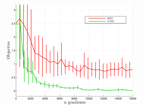
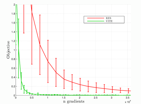
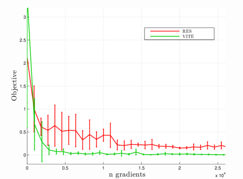
$|{\mathcal{B}}|=0.1\%$
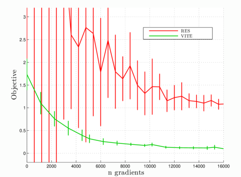
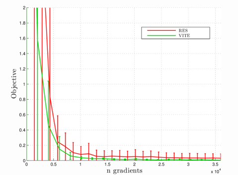
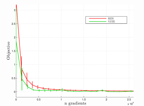
$|{\mathcal{B}}|=2.5\%$
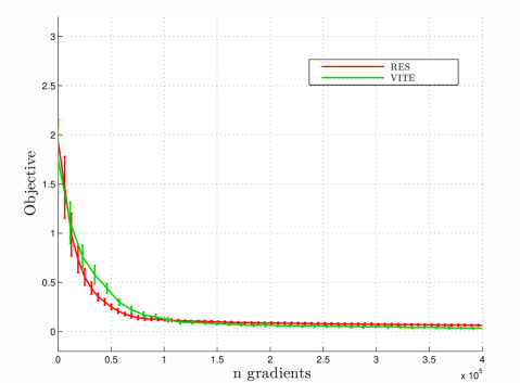
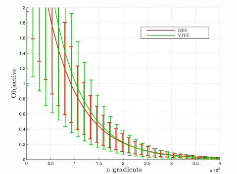
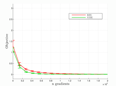
	(a) Cov	(b) Adult	(c) Ijcnn

Figure 1: The red and green curves are the losses achieved by RES and Vite respectively for varying size of $|{\mathcal{B}}|$ as a percentage of $n$. Each experiment was averaged over 5 runs. Error bars denote variance. In the regime $|{\mathcal{B}}|\leq 0.1\%$, Vite has a much lower variance and reaches a lower optimum value. Increasing $|{\mathcal{B}}|$ further decreases the variance of the stochastic gradients but requires more gradient evaluations, decreasing the gap in performance between the methods. Overall, we found VITE with $|{\mathcal{B}}|=1\%$ and $|{\mathcal{B}}|=0.1\%$ to perform the best.

This section presents experimental results that compare the performance of Vite to SGD, SVRG [8] which incorporates variance reduction and RES [12] which incorporates second order information. We consider two commonly occurring problems in machine learning, namely least-square regression and regularized logistic regression.

Linear Least Squares Regression. We apply least-square regression on the binary version of the Cov dataset [4] that contains $n=581,012$ datapoints, each described by $d=54$ input features. Logistic Regression. We apply logistic regression on the Adult and Ijcnn1 datasets obtained from the LibSVM website . The Adult dataset contains $n=32,561$ datapoints, each described by $d=123$ input features. The Ijcnn1 dataset contains $n=49,990$ datapoints, each described by $d=22$ input features. We added an $\ell_{2}$-regularizer with parameter $\lambda=10^{-5}$ to ensure the objective is strongly convex.

The complexity of Vite depends on three quantities: the approximate Hessian $\hat{J}$, the pair of stochastic gradients $(\nabla f_{{\mathcal{B}}}({\bf w}),\nabla f_{{\mathcal{B}}}({\tilde{\bf w}}))$ and $\tilde{\nu}$, respectively computed over the sets ${\mathcal{A}}$, ${\mathcal{B}}$ and ${\mathcal{D}}$. Similarly to [12], we consider different choices for $|{\mathcal{A}}|$ and $|{\mathcal{B}}|$ and pick the best value in a limited interval $\{1,\dots,0.05n\}$. These results are also reported for the RES method that also depends on both $|{\mathcal{A}}|$ and $|{\mathcal{B}}|$. For SGD, we use $|{\mathcal{B}}|=1$ as we found this value to be the best performer on all datasets. Computing the average gradient, $\tilde{\nu}$ over the full dataset for SVRG and Vite is impractical. We therefore estimate $\tilde{\nu}$ over a small subset ${\mathcal{C}}\subset{\mathcal{D}}$. Although this introduces some bias, it did not seem to practically affect convergence for sufficiently large $|{\mathcal{C}}|$. In our experiments, we selected $|{\mathcal{C}}|=0.1n$ samples uniformly at random. Each experiment was averaged over 5 runs with different initializations of ${\bf w}_{0}$ and a random selection of the samples in ${\mathcal{A}}$, ${\mathcal{B}}$ and ${\mathcal{C}}$. Given that the complexity per iteration of each method is different, we compare them as a function of the number of gradient evaluations.

Fig. 1 shows the empirical convergence properties of Vite against RES for least-square regression and logistic regression. The horizontal axis corresponds to the number of gradient evaluations while the vertical axis corresponds to the objective function value. The vertical bars in each plot show the variance over 5 runs. We show plots for different values of $|{\mathcal{B}}|$ and the best corresponding ${\mathcal{A}}$. For small $|{\mathcal{B}}|$, the variance of the stochastic gradients clearly hurts RES while the variance corrections of Vite lead to fast convergence. As we increase $|{\mathcal{B}}|$, thus reducing the variance of the stochastic gradients, the convergence rate of RES and Vite becomes similar. However, Vite with small $|{\mathcal{B}}|$ is much faster to converge to a lower objective value. This clearly demonstrates how using small batches for the computation of the gradients while reducing their variance leads to a fast convergence rate. We also investigated the effect of $|{\mathcal{A}}|$ on the convergence of RES and Vite (see Appendix). In short, we find that a good-enough curvature estimate can be obtained for $|{\mathcal{A}}|=\mathcal{O}(10^{-5}n)$. Increasing this value incurs a penalty in terms of number of gradient evaluations required and so overall performance degrades.

Finally, we compared Vite against SGD, RES and SVRG [8, 9]. A critical factor in the performance of SGD is the selection of the step-size. We use the step-size given in Eq. 2b and pick the parameters $T_{0}$ and $\eta_{0}$ by performing cross-validation over $T_{0}=\{1,10,10^{2},\dots,10^{4}\}$ and $\eta_{0}=\{10^{-1},\dots,10^{-5}\}$. Although it is a quasi-Newton method, RES also requires a decaying step-size and so the same selection process was performed. For SVRG and Vite, we used a constant step size chosen in the same interval as $\eta_{0}$. For SVRG and Vite we used the same size subset, ${\mathcal{C}}$ to compute $\tilde{\nu}$. Fig. 2 shows the objective value of each method in log scale. Although RES and SVRG are superior to SGD, neither clearly outperforms the other. On the other hand, we observe that Vite consistently converges faster than both RES and SVRG. This demonstrates that the combination of second order information and variance reduction is beneficial for fast convergence.

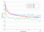
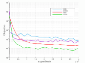
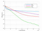
(a) Cov	(b) Adult	(c) Ijcnn

Figure 2: Comparison of RES and Vite (trained with the best performing parameters) against SGD and SVRG. The reduction in variance for Vite is faster than SGD or RES which typically lead to faster convergence.

6 Conclusion

We have shown that stochastic variants of BFGS can be made more robust to the effects of noisy stochastic gradients using variance reduction. We introduced Vite and showed that it obtains a geometric convergence rate for smooth convex functions – to our knowledge the first stochastic Quasi-Newton algorithm with this property. We have shown experimentally that Vite outperforms both variance reduced SGD and stochastic BFGS. The theoretical analysis we present is quite general and additionally only requires that the bound on the eigenvalues of the inverse Hessian matrix in (19) holds. Therefore, the variance reduced framework we propose can be extended to other quasi-Newton methods, including the widely used L-BFGS and AdaGrad [7] algorithms. Finally, an important open question is how to bridge the gap between the theoretical and empirical results. Specifically, whether it is possible to obtain better convergence rates for stochastic BFGS algorithms which match the improvement we have demonstrated over SVRG.

7 Appendix

7.1 Proof of Lemma 2

$${\mathbb{E}} \left|\left|{\bf v}_{t}\right|\right|^{2}={\mathbb{E}}\left|\left|\nabla f_{i}({\bf w}_{t})-\nabla f_{i}({\tilde{\bf w}})+\nabla f({\tilde{\bf w}})\right|\right|^{2}$$

$$\leq 2{\mathbb{E}}\left|\left|\nabla f_{i}({\bf w}_{t})-\nabla f_{i}({\bf w}^{*})\right|\right|^{2}$$

$$+2{\mathbb{E}}\left|\left|(\nabla f_{i}({\tilde{\bf w}})-\nabla f_{i}({\bf w}^{*}))-\nabla f({\tilde{\bf w}})\right|\right|^{2}$$

$$=2{\mathbb{E}}\left|\left|\nabla f_{i}({\bf w}_{t})-\nabla f_{i}({\bf w}^{*})\right|\right|^{2}$$

$$+2{\mathbb{E}}\left|\left|(\nabla f_{i}({\tilde{\bf w}})-\nabla f_{i}({\bf w}^{*}))-(\nabla f({\tilde{\bf w}})-\nabla f({\bf w}^{*}))\right|\right|^{2}$$

$$\leq 2{\mathbb{E}}\left|\left|\nabla f_{i}({\bf w}_{t})-\nabla f_{i}({\bf w}^{*})\right|\right|^{2}$$

$$+2{\mathbb{E}}\left|\left|\nabla f_{i}({\tilde{\bf w}})-\nabla f_{i}({\bf w}^{*})\right|\right|^{2}$$

$$\leq 4L(f({\bf w}_{t})-f({\bf w}^{*})+f({\tilde{\bf w}})-f({\bf w}^{*}))$$ (27)

The second inequality uses ${\mathbb{E}}\left|\left|\xi-{\mathbb{E}}\xi\right|\right|^{2}={\mathbb{E}}\left|\left|\xi\right|\right|^{2}-\left|\left|{\mathbb{E}}\xi\right|\right|^{2}\leq{\mathbb{E}}\left|\left|\xi\right|\right|^{2}$ for any random vector $\xi$.

The last inequality uses the following inequality derived from the fact that $f_{i}$ is a Lipschitz function:

$${\mathbb{E}}\left|\left|\nabla f_{i}({\bf w}^{*})-\nabla f_{i}({\bf w}_{t})\right|\right|^{2}\leq 2L(f({\bf w}_{t})-f({\bf w}^{*})).$$

∎

7.2 Selection of the parameter $|{\mathcal{A}}|$.

Figure 3 shows the effect of the set ${\mathcal{A}}$, used to estimate the inverse Hessian, on the convergence of RES and Vite. We show results for $|{\mathcal{A}}|=\{0.00001,~{}0.0001\}\times n$. Firstly we see that better performance is obtained for both methods for the smaller value of $|{\mathcal{A}}|$. By increasing $|{\mathcal{A}}|$, the penalty paid in terms of gradient evaluations outweighs the gain in terms of better curvature estimates and so convergence is slower. A similar observation was made in [12]. However, we also observe that Vite always outperforms RES for all combinations of $|{\mathcal{A}}|$.

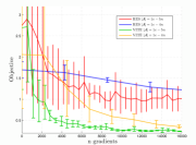
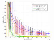
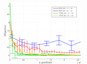
(a) Cov	(b) Adult	(c) Ijcnn

Figure 3: Evolution of the objective value of RES and VITE for different values of $|{\mathcal{A}}|$. We can see that the lowest value of $|{\mathcal{A}}|$ performs better, which indicates than there is no gain at increasing this value passed a certain cut-off value.

References

- [1] F. Bach, E. Moulines, et al. Non-asymptotic analysis of stochastic approximation algorithms for machine learning. In Advances in Neural Information Processing Systems, pages 451–459, 2011.
- [2] L. Bottou. Large-scale machine learning with stochastic gradient descent. In COMPSTAT, pages 177–186. Springer, 2010.
- [3] R. H. Byrd, S. Hansen, J. Nocedal, and Y. Singer. A stochastic quasi-newton method for large-scale optimization. arXiv preprint arXiv:1401.7020, 2014.
- [4] R. Collobert, S. Bengio, and Y. Bengio. A parallel mixture of svms for very large scale problems. Neural computation, 14(5):1105–1114, 2002.
- [5] A. Defazio, F. Bach, and S. Lacoste-Julien. Saga: A fast incremental gradient method with support for non-strongly convex composite objectives. In Advances in Neural Information Processing Systems, pages 1646–1654, 2014.
- [6] J. E. Dennis, Jr and J. J. Moré. Quasi-newton methods, motivation and theory. SIAM review, 19(1):46–89, 1977.
- [7] J. Duchi, E. Hazan, and Y. Singer. Adaptive subgradient methods for online learning and stochastic optimization. The Journal of Machine Learning Research, 12:2121–2159, 2011.
- [8] R. Johnson and T. Zhang. Accelerating stochastic gradient descent using predictive variance reduction. In Advances in Neural Information Processing Systems, pages 315–323, 2013.
- [9] J. Konečnỳ and P. Richtárik. Semi-stochastic gradient descent methods. arXiv preprint arXiv:1312.1666, 2013.
- [10] S. Lacoste-Julien, M. Schmidt, and F. Bach. A simpler approach to obtaining an o (1/t) convergence rate for the projected stochastic subgradient method. arXiv preprint arXiv:1212.2002, 2012.
- [11] D. C. Liu and J. Nocedal. On the limited memory bfgs method for large scale optimization. Mathematical programming, 45(1-3):503–528, 1989.
- [12] A. Mokhtari and A. Ribeiro. Res: Regularized stochastic bfgs algorithm. arXiv preprint arXiv:1401.7625, 2014.
- [13] J. Nocedal and S. Wright. Numerical optimization, volume 2. Springer New York, 1999.
- [14] A. Rakhlin, O. Shamir, and K. Sridharan. Making gradient descent optimal for strongly convex stochastic optimization. arXiv preprint arXiv:1109.5647, 2011.
- [15] H. Robbins and S. Monro. A stochastic approximation method. The annals of mathematical statistics, pages 400–407, 1951.
- [16] N. L. Roux, M. Schmidt, and F. R. Bach. A stochastic gradient method with an exponential convergence rate for finite training sets. In Advances in Neural Information Processing Systems, pages 2663–2671, 2012.
- [17] N. Schraudolph, J. Yu, and S. Günter. A stochastic quasi-newton method for online convex optimization. In Intl. Conf. Artificial Intelligence and Statistics (AIstats), 2007.
- [18] S. Shalev-Shwartz, Y. Singer, N. Srebro, and A. Cotter. Pegasos: Primal estimated sub-gradient solver for svm. Mathematical programming, 127(1):3–30, 2011.