Simultaneous Bidirectional Link Selection in Full Duplex MIMO Systems

Abstract

In this paper, we consider a point to point full duplex (FD) MIMO communication system. We assume that each node is equipped with an arbitrary number of antennas which can be used for transmission or reception. With FD radios, bidirectional information exchange between two nodes can be achieved at the same time. In this paper we design bidirectional link selection schemes by selecting a pair of transmit and receive antenna at both ends for communications in each direction to maximize the weighted sum rate or minimize the weighted sum symbol error rate (SER). The optimal selection schemes require exhaustive search, so they are highly complex. To tackle this problem, we propose a Serial-Max selection algorithm, which approaches the exhaustive search methods with much lower complexity. In the Serial-Max method, the antenna pairs with maximum “obtainable SINR” at both ends are selected in a two-step serial way. The performance of the proposed Serial-Max method is analyzed, and the closed-form expressions of the average weighted sum rate and the weighted sum SER are derived. The analysis is validated by simulations. Both analytical and simulation results show that as the number of antennas increases, the Serial-Max method approaches the performance of the exhaustive-search schemes in terms of sum rate and sum SER.

I Introduction

Current wireless communications systems typically exploit half duplex (HD) transmission. This is because for many years the full duplex (FD) transmission has been considered impractical. The signal leakage from the local output to input in the FD radio, referred to as the self interference, may overwhelm the receiver, thus making it impossible to extract the desired signals. Very recently, there has been a significant process in self-interference suppression in FD radios. The passive suppression methods [1, 2, 6, 8, 4, 7, 3, 5] design the antennas using a combination of path loss, cross polarization and antenna directionality, while the active approaches [1, 9, 10, 6, 8, 3] exploit the knowledge of self interference in cancelation in the analog or digital domain. The residual interference still exists and can be modeled as Rayleigh fading [3, 17, 16] when the direct link is effectively suppressed.

These suppression techniques can significantly reduce the self-interference, which has made FD radios practically feasible in the near future. This significant progress in FD has recently inspired some very interesting work on FD signal processing. In [8, 12, 15, 11, 14, 13], the theoretical limits of point to point bidirectional FD have been investigated by taking into account the residual self-interference after suppression. In [8], the authors derived lower and upper bounds of the achievable sum rate of bidirectional FD communications, and proposed a transmission scheme to maximize the lower bound. In [11], the achievable sum rate of bidirectional FD MIMO systems was analyzed and compared to the conventional HD MIMO systems over a spatial correlated channel. The ergodic capacity of bidirectional FD transmission using one transmit antenna and multiple receive antennas in the presence of channel estimation error has been derived in [12]. a FD antenna mode selection scheme was investigated in [13] for a simple $2\times 2$ MIMO system, where each antenna is either configured as the transmit or receive antenna mode. In [15, 14], the suboptimal and optimal dynamic power allocation schemes were developed based on the sum rate maximization criterion.

In this paper, we consider a general FD MIMO system with $N_{A}$ and $N_{B}$ antennas equipped at two nodes. Such an FD MIMO system will create $N_{A}N_{B}$ possible links between the two FD MIMO nodes, with one possible link representing the channel from a transmit antenna of a node to a receive antenna of the other node. Since FD radios enable simultaneous bidirectional information exchanges between two FD MIMO nodes, a fundamental question arisen in such a system is how to select the link for each direction to optimize the system performance. In this paper we consider two performance metrics, weighted sum rate maximization and weighted sum symbol error rate (SER) minimization. The optimal approach requires the exhaustive search from all possible antenna links, however, as the number of antennas increases, such a brute-force search bears very high complexity in selection process.

To resolve this issue, in this paper we propose a simple Serial-Max selection algorithm by selecting the link with optimal performance for each direction in a two-step serial way, which can achieve asymptotically optimal performance. By using the law of total probability and order statics, the probability distribution functions of the two selected links are calculated, based on which, the closed-form expressions on average weighted sum rate and sum SER are derived. We show that the Serial-Max method approaches the brute-force search method in terms of the average weighted sum rate and sum SER as the number of antennas increases. The theoretical results are verified by Monte-Carlo simulations.

The rest of this paper is organized as follows: Section II introduces the system model. The proposed Serial-Max selection algorithm is presented in Section III. Section IV analyzes the performance of the Serial-Max method, including the average weighted sum rate and sum SER. Simulation results are provided in Section V. In Section VI, we draw the main conclusions.

II System Model

In this paper, we consider a bidirectional communication scenario between a pair of FD transceivers, node $A$ and $B$, as illustrated in Fig. 1, where node $A$ and $B$ are equipped with $N_{A}$ and $N_{B}$ antennas, respectively. Both nodes use the same frequency band at the same time for FD operation. Each node employs only one transmit and one receive RF chains, and any antenna can be configured to connect either the transmit or receive RF chain. In the proposed simultaneous bidirectional link selection (SBLS) scheme, two antenna links are selected for simultaneous bidirectional communication by selecting a pair of transmit and receive antennas at both ends. Within each antenna pair, one antenna is selected for transmission and one is for reception.

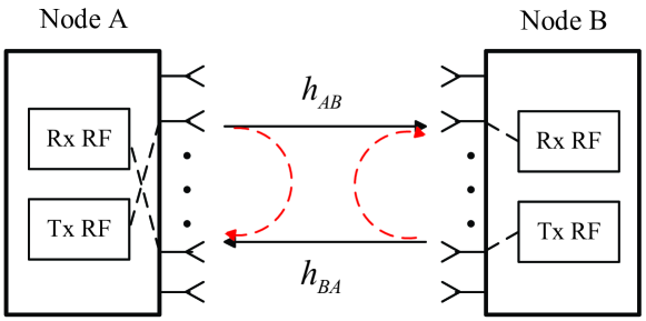
Figure 1: Full duplex MIMO systems with simultaneous bidirectional link selection

We assume that the links between the two nodes are reciprocal and subject to independent Rayleigh fading, and together denoted by a $N_{A}\times N_{B}$ channel matrix ${\bf H}=\left[h^{ij}\right],i=1,2,...,N_{A},j=1,2,...,N_{B}$. The entry $h^{ij}$ represents the fading coefficient from the $i$-th antenna at node $A$ to the $j$-th antenna at node $B$, and it follows the circularly symmetric Gaussian distribution $\mathcal{C}\mathcal{N}(0,\sigma_{h}^{2})$. All the possible communication channels are assumed to follow the non-selective independent block fading, where the channel coefficients remain constant during a time slot, and vary from one to another independently. In the beginning of each time slot, all the possible communication links can be estimated perfectly.

Since the two nodes are operated in the FD mode, there exists self interference caused by the signal leakage from the transmit antenna to the receive antenna at the same node. We assume the passive propagation suppression and active analog/digital cancelation techniques are employed to cancel the self interference. As indicated in [17, 16], the direct link of the self interference can be effectively suppressed, and the residual self interference can be approximated to follow the Rayleigh distribution [20, 21]. In this paper, due to practical constraints, we assume that only the distribution of the residual interference, including the mean and variance, can be obtained and used in the selection process. Therefore, the selection process is based on the “obtainable SINR”. This is equivalent to that based on the instantaneous SNR, which will be later shown that the former is a scaled version of the latter.

In the SBLS, the bidirectional links, i.e., $(I_{T},J_{R})$, from the $I_{T}$-th antenna at node $A$ to the $J_{R}$-th antenna at node $B$, and $(J_{T},I_{R})$, from the $J_{T}$-th antenna at node $B$ to the $I_{R}$-th antenna at node $A$, are selected. The received signals at node $A$ and $B$, denoted by $y_{A}$ and $y_{B}$, can be expressed as

$${y_{A}}= \sqrt{{P_{t}}}{h^{J_{T}I_{R}}}{x_{B}}+\sqrt{{P_{t}}}{h^{RI}_{A}}x_{A}+{n_{A}}$$ (1)

$${y_{B}}= \sqrt{{P_{t}}}{h^{I_{T}J_{R}}}{x_{A}}+\sqrt{{P_{t}}}h^{RI}_{B}{x_{B}}+{n_{B}},$$

where $h^{I_{T}J_{R}}$ and $h^{J_{T}I_{R}}$ denote the links corresponding to the selected antenna pair from node $A$ to $B$ and that from node $B$ to $A$. $P_{t}$ is the transmit power at each node. The second term denotes the residual interference, at nodes $A$ and $B$, respectively. We assume that both residual interference links, $h_{A}^{RI}$ and $h_{B}^{RI}$, are subject to Rayleigh fading with zero mean and variance $\sigma_{RI}^{2}$. The AWGN at nodes $A$ and $B$ are denoted by $n_{A}$ and $n_{B}$, which both follow $\mathcal{C}\mathcal{N}(0,\sigma_{n}^{2})$.

Without the knowledge of the instantaneous residual interference, the selection procedure is based on the “obtainable SINR” matrix ${\bf\Gamma}=[\gamma^{ij}]$. The entry in the “obtainable SINR” matrix is defined as $\gamma^{ij}=\frac{\gamma^{ij}_{s}}{(\lambda_{i}+1)}$, where $\gamma^{ij}_{s}=\frac{P_{t}|h^{ij}|^{2}}{\sigma_{n}^{2}}$ is the instantaneous SNR, and $\lambda_{i}$ is the average INR. $\gamma^{ij}_{s}$ follows an exponential distribution with mean $\lambda_{s}=\frac{P_{t}\sigma_{h}^{2}}{\sigma_{n}^{2}}$, and the average INR is given by $\lambda_{i}=\eta\lambda_{s}=\frac{P_{t}\sigma_{RI}^{2}}{\sigma_{n}^{2}}$, where $\eta$ denotes the cancelation ability. The “obtainable SINR” $\gamma^{ij}$ is a scaled version of the instantaneous SNR $\gamma^{ij}_{s}$, because we assume that all the links have the same average INR $\lambda_{i}$.

In the following analysis in Section IV, we first calculate the instantaneous performance based on the instantaneous residual interference, and then average it with the distribution of fading channel and residual interference channel. We define the instantaneous SINR $\gamma_{AB}=\frac{\gamma_{s}^{I_{T}J_{R}}}{\gamma^{RI}_{B}+1}$ and $\gamma_{BA}=\frac{\gamma_{s}^{J_{T}I_{R}}}{\gamma^{RI}_{A}+1}$ for the two selected links. where the instantaneous INR $\gamma^{RI}_{A}$ and $\gamma^{RI}_{B}$ are both exponential random variables with mean $\lambda_{i}$.

III Simultaneous Bidirectional Link Selection (SBLS)

In this section, we first introduce two optimal SBLS approaches to maximize the weighted sum rate and minimize the weighted sum SER, respectively, based on the “obtainable SINR” matrix, or equivalently the SNR matrix. Then, a low-complexity method which achieves asymptotically optimal performance, referred to as Serial-Max method, is proposed.

III-A SBLS based on Weighted Sum Rate Maximization Criterion (Max-WSR)

In this subsection, we describe the SBLS based on Weighted Sum Rate Maximization criterion (Max-WSR) under the Gaussian input assumption. In this criterion, two communication links $\{(I_{T},J_{R}),(I_{R},J_{T})\}$ from the $I_{T}$-th transmit antenna at node $A$ to the $J_{R}$-th receive antenna at node $B$ and the $J_{T}$-th transmit antenna at node $B$ to the $I_{R}$-th receive antenna at node $A$, are selected to maximize the weighted bidirectional sum rate

$$\left\{{({I_{T}},{J_{R}}),({I_{R}},{J_{T}})}\right\}=\mathop{\arg\max}\limits_{\scriptstyle{\kern 1.5pt}1\leq{i_{t}},{i_{r}}\leq N_{A}\hfill\atop{\scriptstyle 1\leq{j_{t}},{j_{r}}\leq N_{B}\hfill\atop\scriptstyle{i_{t}}\neq{i_{r}},{j_{t}}\neq{j_{r}}\hfill}}\left\{wR\left({\gamma^{{i_{t}}{j_{r}}}}\right)+(1-w)R\left({{\gamma^{{i_{r}}{j_{t}}}}}\right)\right\},$$ (2)

where $R(\gamma)=\log_{2}\left[1+\gamma\right]$ denotes the rate under the “obtainable SINR” $\gamma=\frac{\gamma_{s}}{(\lambda_{i}+1)}$, and $0<w<1$ is the given weight of the transmission from node $A$ to $B$, depending on the rate requirement or quality of service (QoS) of each user.

III-B SBLS Based on Weighted Sum SER Minimization (Min-WSER)

In the SBLS based on weighted sum SER minimization criterion (Min-WSER) under the assumption that the input signal is modulated with finite constellations, the bidirectional antenna links are selected to minimize the weighted sum SER

$$\left\{{({I_{T}},{J_{R}}),({I_{R}},{J_{T}})}\right\}=\mathop{\arg\min}\limits_{\scriptstyle{\kern 1.0pt}1\leq{i_{t}},{i_{r}}\leq N_{A}\hfill\atop{\scriptstyle 1\leq{j_{t}},{j_{r}}\leq N_{B}\hfill\atop\scriptstyle{i_{t}}\neq{i_{r}},{j_{t}}\neq{j_{r}}\hfill}}\left\{w{SE{R}\left({{{{\gamma^{{i_{r}}{j_{t}}}}}}}\right)}{+(1-w)SE{R}\left({{{{\gamma^{{i_{t}}{j_{r}}}}}}}\right)}\right\},$$ (3)

where ${SE{R}\left(\gamma\right)}=\alpha Q\left({\sqrt{\beta\gamma}}\right)$ represents the SER under the “obtainable SINR” $\gamma=\frac{\gamma_{s}}{(\lambda_{i}+1)}$. $Q(\cdot)$ is the Gaussian $Q$-function [22], and $(\alpha,\beta)$ is a pair of constants determined by the modulation format, e.g., $\alpha=1,\beta=2$ for BPSK modulation.

III-C The Proposed Serial-Max SBLS

The aforementioned SBLS schemes for the Max-WSR or Min-WSER criteria both require the brute-force search in order to find the optimal antenna pairs. This will become highly complex in selection process as the number of antennas increases. In this subsection, we introduce a low-complexity selection method, referred to as Serial-Max method, which selects the antenna pairs with maximum “obtainable SINR”, or equivalently, the maximum SNR, in a two-step serial way.

In the first step, the best link with the maximum “obtainable SINR” is selected

$$({I_{1}},{J_{1}})=\mathop{\arg\max}\limits_{1\leq{i_{1}}\leq N_{A},1\leq{j_{1}}\leq N_{B}}\left\{{{\gamma^{{i_{1}}{j_{1}}}}}\right\}.$$ (4)

We use $\gamma^{1st}\buildrel\Delta\over{=}{\gamma^{{I_{1}}{J_{1}}}}$ to denote the “obtainable SINR” of the selected link $({I_{1}},{J_{1}})$, and $\gamma^{1st}_{s}$ to denote the SNR of this link. By removing the $I_{1}$-th column and $J_{1}$-th row from the “obtainable SINR” matrix $\bf\Gamma$ (and the corresponding SNR matrix $\bf\Gamma_{s}$), we can obtain a $(N_{A}-1)\times(N_{B}-1)$ submatrix $\bf\Gamma^{\prime}$ (and a corresponding pruned SNR matrix $\bf\Gamma^{\prime}_{s}$).

In the second step, the link $(I_{2},J_{2})$ with the maximum SNR is then selected from the pruned submatrix $\bf\Gamma^{\prime}$

$$({I_{2}},{J_{2}})=\mathop{\arg\max}\limits_{\scriptstyle{1\leq{i_{2}}\leq N_{A},1\leq{j_{2}}\leq N_{B}}\hfill\atop\scriptstyle\hskip 14.22636pt{i_{2}}\neq{I_{1}},{j_{2}}\neq{J_{1}}\hfill}\left\{{{\gamma^{{i_{r}}{j_{t}}}}}\right\}.$$ (5)

We use $\gamma^{2nd}\buildrel\Delta\over{=}{\gamma^{{I_{2}}{J_{2}}}}$ to denote the “obtainable SINR” of the second selected link by the Serial-Max method, which is the maximum element of $\bf\Gamma^{\prime}$, and we use $\gamma^{2nd}_{s}$ to denote the SNR of this link, which is the maximum element of the corresponding pruned SNR matrix $\bf\Gamma^{\prime}_{s}$.

To maximize the weighted sum rate or minimize the weighted sum SER, the time-shared scheme can be employed, which allocates a fraction $\alpha$ of the time to use the best link for node $A$’s transmission, and the rest $1-\alpha$ to use the best link for node $B$’s transmission. Given $w$, the weighted maximization sum rate problem can be solved by calculating the allocation fraction $\alpha$. We have

$$R=w\left[{\alpha R\left({\gamma^{1st}}\right)+\left({1-\alpha}\right)R\left({\gamma^{2nd}}\right)}\right]+(1-w)\left[{\alpha R\left({\gamma^{2nd}}\right)+\left({1-\alpha}\right)R\left({\gamma^{1st}}\right)}\right].$$ (6)

To maximize $R$, we first calculate the derivative

$$\frac{{\partial R}}{{\partial\alpha}}=\left(2w-1\right)\left[R\left({\gamma^{1st}}\right)-R\left({\gamma^{2nd}}\right)\right].$$ (7)

It is obvious that $R\left({\gamma^{1st}}\right)-R\left({\gamma^{2nd}}\right)$ is positive, therefore the allocation factor $\alpha$ depends on wether $w>0.5$ or not. Specifically, we have

$$\left\{\begin{array}[]{l}\alpha=1,{\kern 27.0pt}w>0.5\\ \alpha=0,{\kern 27.0pt}w<0.5\\ 0\leq\alpha\leq 1,{\kern 6.0pt}w=0.5\end{array}\right..$$ (8)

Then, the weighted sum rate can be rewritten as

$$R=\max(w,1-w)R\left({\gamma^{1st}}\right)+\min(w,1-w){{R}\left({\gamma^{2nd}}\right)},$$ (9)

The weighted sum SER minimization problem can be solved in a similar way, and we have

$$SER=\max(w,1-w)SER\left({\gamma^{1st}}\right)+\min(w,1-w){{SER}\left({\gamma^{2nd}}\right)}.$$ (10)

It is shown from (9) and (10) that the best link selected in the Serial-Max method will be allocated with the greater weight in the weighted sum rate and SER expression.

Regarding the performance of the Serial-Max method, we have the following Lemma.

Lemma 1: The Serial-Max method can achieve the optimal weighted sum rate and sum SER performances simultaneously, if the “obtainable SINR” of the second selected link $\gamma^{2nd}$ is the second or third largest element of the “obtainable SINR” matrix $\bf\Gamma$.

Proof: We use $R_{i}$ and $SER_{i}$ to denote the respective rate and SER of the link with the $i$-th largest “obtainable SINR”. If the second selected link corresponds to the second largest element in the “obtainable SINR” matrix $\bf\Gamma$, the weighted sum rate is given by $R=\max(w,1-w)R_{1}+\min(w,1-w)R_{2}$. It is obvious that in this case the Serial-Max method can achieve the optimal performance in terms of weighted sum rate. Similarly, it can be easily proved that the Serial-Max method can achieve the optimal performance of SER.

Recall that the pruned matrix $\bf\Gamma^{\prime}$ is obtained by removing the row and column where the largest element, i.e., the first selected link, is located. Meanwhile, the second selected link is the largest element of the pruned matrix $\bf\Gamma^{\prime}$. Therefore, if the second selected link corresponds to the third largest element in the original “obtainable SINR” matrix, it implies that the second largest element in $\bf\Gamma$ is removed in the aforementioned manipulation. In other words, the two links associated with the first and second largest elements in $\bf\Gamma$ share the same antenna, which can not be selected simultaneously. In this case, the largest and third largest elements is the best option for the two selected links. Therefore, the Serial-Max method which selects the largest and third largest elements in $\bf\Gamma$ achieves the optimal performances of weighted sum rate and sum SER. $\hfill\blacksquare$

Then, we have the following proposition.

Proposition 1: The probability that the Serial-Max method does not achieve the same performance as the optimal methods, denoted by $P_{not}$, is upper bounded by

$$P_{not}\leq\frac{{\left({{N_{A}}+{N_{B}}-2}\right)\left({{N_{A}}+{N_{B}}-3}\right)}}{{\left({{N_{A}}{N_{B}}-1}\right)\left({{N_{A}}{N_{B}}-2}\right)}}.$$ (11)

Proof: According to Lemma 1, $P_{not}$ is upper bounded by the probability, denoted by $P_{not}^{2,3}$, that the “obtainable SINR” of the second selected link $\gamma^{2nd}$ is not the second nor third largest elements of the “obtainable SINR” matrix $\bf\Gamma$. This implies that both the second and third largest elements are in the same row or column as the largest element, and they are both removed in the process of obtaining the pruned “obtainable SINR” matrix $\bf\Gamma^{\prime}$. Note that the elements of $\bf\Gamma$ are independent and identically distributed. Due to symmetry, each element of $\bf\Gamma$ has the same probability to be the $i$-th largest element. Thus, we have

$$P_{not}^{2,3}=\frac{{\left({{N_{A}}+{N_{B}}-2}\right)\left({{N_{A}}+{N_{B}}-3}\right)}}{{\left({{N_{A}}{N_{B}}-1}\right)\left({{N_{A}}{N_{B}}-2}\right)}}.$$ (12)

Combining the fact that $P_{not}$ is no more than $P_{not}^{2,3}$, Proposition 1 can be proved. $\hfill\blacksquare$

It is shown from (11) that the upper bound of $P_{not}$ decreases quadratically as the number of antennas increases, which implies the probability that the Serial-Max method selects the same pairs as the optimal one will increase, and thus approaches the optimal performance in terms of weighted sum rate and sum SER asymptotically.

In addition to the asymptotically-optimal performance, the complexity of the Serial-Max method is much simpler than the exhaustive search approach, as shown in Table I. For the Serial-Max method, in the first step, the maximum “obtainable SINR” is selected from a $N_{A}\times N_{B}$ matrix, and ${N_{A}N_{B}}$ comparisons are required. Similarly, for the second step $(N_{A}-1)(N_{B}-1)$ comparisons are needed, and the Serial method overall needs $2{N_{A}N_{B}}-N_{A}-N_{B}+1$ comparisons. By contrary, the optimal method requires exhaustive search in order to find the optimal antenna pairs, leading to $\frac{N_{A}N_{B}(N_{A}-1)(N_{B}-1)}{2}$ comparisons. Therefore, the proposed Serial-Max algorithm can approach the optimal algorithm with significantly reduced complexity.

TABLE I: Complexity comparison

	Optimal selection approach	Serial-Max approach
Complexity	$\frac{N_{A}N_{B}(N_{A}-1)(N_{B}-1)}{2}$	$2{N_{A}N_{B}}-N_{A}-N_{B}+1$

IV Performance Analysis

The optimal selection methods are both very difficult to analyze, and thus, in this section we analyze the performance of the Serial-Max algorithm. It will be shown later in simulations that the Serial-Max method can achieve near-optimal performance in terms of average weighted sum rate and SER.

IV-A Probability Distributions of Two Selected Links

To analyze the performances of the Serial-Max method, the distributions of the real instantaneous SINR corresponding to the two selected links $\gamma_{AB}$ and $\gamma_{BA}$ are required. For simplicity and without loss of generality, we consider the case of $w>0.5$ for the following analysis, which can be easily extended to $w\leq 0.5$.

According to the description of the Serial-Max method in (4), the SNR of the first selected link, $\gamma^{1st}_{s}$ is the largest order statistic among ${N_{A}N_{B}}$ i.i.d. exponentially distributed random variables $\gamma^{ij}_{s}$. The corresponding link $(I_{1},J_{1})$ is used for transmission from node $A$ to $B$. We have the following Lemma.

Lemma 2: The CDF of $\gamma_{AB}$ can be given by

$${F_{\gamma_{AB}}}(x)=\sum\limits_{k=0}^{{N_{A}}{N_{B}}}{\binom{N_{A}N_{B}}{k}{{\left({-1}\right)}^{k}}\frac{{e^{-\frac{k}{{{\lambda_{s}}}}x}}}{{k\eta x+1}}}.$$ (13)

Proof: The derivation is given in Appendix A. $\hfill\blacksquare$

The second selected link in the Serial-Max method $(I_{2},J_{2})$ is used for transmission from node $B$ to $A$. According to (5), we can obtain

Lemma 3: The CDF expression of the instantaneous link SINR of the second selected link, i.e., $\gamma_{BA}$, is given by

$${F_{{\gamma_{BA}}}}(x)=\sum\limits_{k=1}^{{N_{A}}+{N_{B}}-1}{\sum\limits_{l={N_{A}}{N_{B}}-k}^{{N_{A}}{N_{B}}}{\sum\limits_{m=0}^{l}{{{\left({-1}\right)}^{m}}{\mu_{k,l,m}}}\frac{{e^{-\frac{{{N_{A}}{N_{B}}-l+m}}{{{\lambda_{s}}}}x}}}{{\left({{N_{A}}{N_{B}}-l+m}\right)\eta x+1}}}},$$ (14)

where $\mu_{k,l,m}$ is expressed as

$$\mu_{k,l,m}=\frac{\binom{{N_{A}N_{B}}-k-1}{N_{A}+N_{B}-k-1}\binom{{N_{A}N_{B}}}{l}\binom{l}{m}}{\binom{{N_{A}N_{B}}-1}{N_{A}+N_{B}-2}}.$$ (15)

Proof: The derivation is given in Appendix B. $\hfill\blacksquare$

IV-B Average weighted Sum Rate

Based on the CDF expressions of the two selected links $\gamma_{AB}$ and $\gamma_{BA}$, in this section, the average weighted sum rate of the two links is obtained. Firstly, the instantaneous rate is calculated for given realizations of the selected communication channel and the corresponding self-interference channel. Then the average rate is obtained by averaging the instantaneous rate with respect to the distributions of the channels. Under the Gaussian input assumption, the average rate of the link with SINR $\gamma$ can be obtained as

$$\bar{R} =\mathbb{E}\left[\log_{2}(1+\gamma)\right]$$ (16)

$$=\frac{1}{{\ln 2}}\int\limits_{0}^{\infty}{\frac{{1-{F_{\gamma}}(x)}}{{1+x}}}dx,$$

where $F_{\gamma}(x)$ is the CDF of $\gamma$.

Proposition 2: The average weighted sum rate of the Serial-Max method, denoted by $\bar{R}^{S-Max}$ is given by

$$\bar{R}^{S-Max}=w\bar{R}_{AB}+(1-w){{\bar{R}}_{BA}},$$ (17)

where $\bar{R}_{AB}$ and $\bar{R}_{BA}$ are the average rates of the two selected links, respectively, which can be expressed as

$${{\bar{R}}_{AB}}=\frac{1}{{\ln 2}}\sum\limits_{k=0}^{{N_{A}}{N_{B}}}{\frac{{{{\left({-1}\right)}^{k}}\binom{N_{A}N_{B}}{k}}}{{1-k\eta}}\left[{{e^{\frac{1}{{\eta{\lambda_{s}}}}}}{{\rm{E}}_{1}}\left({\frac{1}{{\eta{\lambda_{s}}}}}\right)-{e^{\frac{k}{{{\lambda_{s}}}}}}{{\rm{E}}_{1}}\left({\frac{k}{{{\lambda_{s}}}}}\right)}\right]},$$ (18)

and

$${{\bar{R}}_{BA}}=\frac{1}{{\ln 2}}\sum\limits_{k=1}^{{N_{A}}+N_{B}-1}{\left({{F_{1}}+{F_{2}}}\right)},$$ (19)

where

$${F_{1}}=\sum\limits_{l={N_{A}}{N_{B}}-k}^{{N_{A}}{N_{B}}-1}{\sum\limits_{m=0}^{l}{\frac{{{{\left({-1}\right)}^{m}}{\mu_{k,l,m}}}}{{1-\left({{N_{A}}{N_{B}}-l+m}\right)\eta}}\left[{{e^{\frac{1}{{\eta{\lambda_{s}}}}}}{{\rm{E}}_{1}}\left({\frac{1}{{\eta{\lambda_{s}}}}}\right)-{e^{\frac{{{N_{A}}{N_{B}}-l+m}}{{{\lambda_{s}}}}}}{{\rm{E}}_{1}}\left({\frac{{{N_{A}}{N_{B}}-l+m}}{{{\lambda_{s}}}}}\right)}\right]}},$$ (20)

and

$${F_{2}}=\sum\limits_{m=1}^{{N_{A}}{N_{B}}}{\frac{{{{\left({-1}\right)}^{m+1}}{\mu_{k,{N_{A}}{N_{B}},m}}}}{{1-m\eta}}\left[{{e^{\frac{1}{{\eta{\lambda_{s}}}}}}{{\rm{E}}_{1}}\left({\frac{1}{{\eta{\lambda_{s}}}}}\right)-{e^{\frac{m}{{{\lambda_{s}}}}}}{{\rm{E}}_{1}}\left({\frac{m}{{{\lambda_{s}}}}}\right)}\right]}.$$ (21)

In addition, ${\rm E}_{1}(\cdot)$ denotes the exponential integral function [22].

Proof: The derivation is given in Appendix C. $\hfill\blacksquare$

It is shown from (17)–(21) that the average weighted sum rate of the Serial-Max method $\bar{R}^{S-Max}$ is only determined by the average SNR $\lambda_{s}$ and cancelation ability $\eta$. When $\lambda_{s}$ goes to infinity, we have ${\rm E}_{1}(\varepsilon)\approx-\gamma-\ln(\varepsilon)$ and $e^{\varepsilon}\approx 1+\varepsilon$, for $\varepsilon=1/\lambda_{s}$, where $\gamma\approx 0.5772$ is Euler’s constant [28]. After some manipulations, $\bar{R}^{S-Max}$ converges to a rate ceiling ${{\bar{R}}^{S-Max}}_{\lambda\rightarrow\infty}$

$$\bar{R}_{\lambda_{s}\rightarrow\infty}^{S-Max}\rightarrow\frac{w}{{\ln 2}}\sum\limits_{k=0}^{{N_{A}}{N_{B}}}{\frac{{{{\left({-1}\right)}^{k}}\binom{N_{A}N_{B}}{k}\ln\left({k\eta}\right)}}{{1-k\eta}}+\frac{{1-w}}{{\ln 2}}\sum\limits_{k=1}^{{N_{A}}+{N_{B}}-1}{\sum\limits_{m=1}^{{N_{A}}{N_{B}}}{\frac{{{{\left({-1}\right)}^{m}}{\mu_{k,{N_{A}}{N_{B}},m}}\ln\left({m\eta}\right)}}{{1-m\eta}}}}}$$ (22)

$$+\frac{{1-w}}{{\ln 2}}\sum\limits_{k=1}^{{N_{A}}+{N_{B}}-1}{\sum\limits_{l={N_{A}}{N_{B}}-k}^{{N_{A}}{N_{B}}-1}{\sum\limits_{m=0}^{l}{\frac{{{{\left({-1}\right)}^{m}}{\mu_{k,l,m}}\ln\left[{\left({{N_{A}}{N_{B}}-l+m}\right)\eta}\right]}}{{1-\left({{N_{A}}{N_{B}}-l+m}\right)\eta}}}}}$$

IV-C Average weighted sum SER

In this section, we analyze the average weighted sum SER of the Serial-Max method. For the SER analysis, we assume that the input signal is modulated with a finite constellation. Though the finite constellations like BPSK are used, the current self-interference cancellation technique can reduce the self-interference near to the noise level, as shown in [24, 17]. It has thus been commonly assumed in many existing papers that the residual self-interference after cancellation follow the Rayleigh distributions [16, 20]. We also adopt this assumption in this paper. Firstly, the SER is calculated for a given set of channel realizations, similar to the weighted sum rate analysis. Then, the SER is averaged over the communication and self-interference channels. The average SER of the link with SINR $\gamma$ can be written as

$$\overline{SER} =\alpha\mathbb{E}\left[Q\left(\sqrt{\beta\gamma}\right)\right]$$ (23)

$$=\frac{\alpha\sqrt{\beta}}{{2\sqrt{2\pi}}}\int\limits_{0}^{\infty}\frac{F_{\gamma}\left(x\right)e^{-\frac{{\beta x}}{2}}}{\sqrt{x}}dx.$$

$Q(\cdot)$ is the Gaussian Q-Function [22].

In addition, if the first-order expansion of the PDF of $\gamma$ is expressed as

$$f_{\gamma}(x)=\frac{\zeta x^{N}}{\lambda^{N+1}}+o(x^{N+\varepsilon}),$$ (24)

the asymptotic SER can be obtained as [25, 26]

$$\overline{SER}=\frac{{{2^{N}}\alpha\zeta\Gamma\left({N+\frac{3}{2}}\right)}}{{\sqrt{\pi}\left({N+1}\right){{\left({\beta\lambda}\right)}^{N+1}}}}+o\left({\frac{1}{{{{\lambda}^{\left({N+1}\right)}}}}}\right).$$ (25)

Proposition 3: The average weighted sum SER of the Serial-Max method, denoted by ${\overline{SER}^{S-Max}}$ is

$${\overline{SER}^{S-Max}}=w{\overline{SER}_{AB}}+(1-w){\overline{SER}_{BA}},$$ (26)

where ${\overline{SER}_{AB}}$ and ${\overline{SER}_{BA}}$ are the average SER of the two selected links, and can be calculated as

$${\overline{SER}_{AB}}=\frac{1}{2}+\frac{{\alpha\sqrt{\beta\pi}}}{{\sqrt{2}}}\sum\limits_{k=1}^{{N_{A}}{N_{B}}}{\frac{{{{(-1)}^{k}}\binom{N_{A}N_{B}}{k}}}{{\sqrt{k\eta}}}{Q}\left({\sqrt{\frac{2}{{\eta{\lambda_{s}}}}+\frac{\beta}{{k\eta}}}}\right)}{e^{\frac{1}{{\eta{\lambda_{s}}}}+\frac{\beta}{{2k\eta}}}},$$ (27)

and

$${\overline{SER}_{BA}}=\frac{{\alpha\sqrt{\beta\pi}}}{{\sqrt{2}}}\sum\limits_{k=1}^{{N_{A}}+{N_{B}}-1}{\left({{G_{1}}+{G_{2}}}\right)},$$ (28)

where

$${G_{1}}=\sum\limits_{l={N_{A}}{N_{B}}-k}^{{N_{A}}{N_{B}}-1}{\sum\limits_{m=0}^{l}{\frac{{{{\left({-1}\right)}^{m}}{\mu_{k,l,m}}}}{{\sqrt{\left({{N_{A}}{N_{B}}-l+m}\right)\eta}}}{Q}\left({\sqrt{\frac{2}{{\eta{\lambda_{s}}}}+\frac{\beta}{{\left({{N_{A}}{N_{B}}-l+m}\right)\eta}}}}\right){e^{\frac{1}{{\eta{\lambda_{s}}}}+\frac{\beta}{{2\left({{N_{A}}{N_{B}}-l+m}\right)\eta}}}}}},$$ (29)

and

$${G_{2}}=\sum\limits_{m=1}^{{N_{A}}{N_{B}}}{\frac{{{{\left({-1}\right)}^{m}}{\mu_{k,{N_{A}}{N_{B}},m}}}}{{\sqrt{m\eta}}}{Q}\left({\sqrt{\frac{2}{{\eta{\lambda_{s}}}}+\frac{\beta}{{m\eta}}}}\right){e^{\frac{1}{{\eta{\lambda_{s}}}}+\frac{\beta}{{2m\eta}}}}}.$$ (30)

Proof: The derivation is given in Appendix D. $\hfill\blacksquare$

The SER performance converges to an error floor, when the average SNR $\lambda_{s}$ increases to infinity

$$\overline{SER}_{\lambda\rightarrow\infty}^{S-Max}\rightarrow 1-\frac{{w\alpha\sqrt{\beta\pi}}}{{\sqrt{2}}}\sum\limits_{k=1}^{{N_{A}}{N_{B}}}{\frac{{{{(-1)}^{k+1}}\binom{N_{A}N_{B}}{k}}}{{\sqrt{k\eta}}}{Q}\left({\sqrt{\frac{\beta}{{k\eta}}}}\right){e^{\frac{\beta}{{2k\eta}}}}}$$ (31)

$$-\frac{{\left({1-w}\right)\alpha\sqrt{\beta\pi}}}{{\sqrt{2}}}\sum\limits_{k=1}^{{N_{A}}+{N_{B}}-1}{\frac{{{{\left({-1}\right)}^{m+1}}{\mu_{k,{N_{A}}{N_{B}},m}}}}{{\sqrt{m\eta}}}{Q}\left({\sqrt{\frac{\beta}{{m\eta}}}}\right){e^{\frac{\beta}{{2m\eta}}}}}$$

$$-\frac{{\left({1-w}\right)\alpha\sqrt{\beta\pi}}}{{\sqrt{2}}}\sum\limits_{k=1}^{{N_{A}}+{N_{B}}-1}{\sum\limits_{l={N_{A}}{N_{B}}-k}^{{N_{A}}{N_{B}}}{\sum\limits_{m=0}^{l}{\frac{{{{\left({-1}\right)}^{m+1}}{\mu_{k,l,m}}}}{{\sqrt{\left({{N_{A}}{N_{B}}-l+m}\right)\eta}}}}}}$$

$${\hskip 14.22636pt}\times{Q}\left({\sqrt{\frac{\beta}{{\left({{N_{A}}{N_{B}}-l+m}\right)\eta}}}}\right){e^{\frac{\beta}{{2\left({{N_{A}}{N_{B}}-l+m}\right)\eta}}}}.$$

On the other hand, when $\eta=0$, i.e. the self interference is perfectly canceled, we can further calculate the asymptotic SER of the Serial-Max method at high SNR. Firstly, the CDF expression of $\gamma_{AB}$ can be rewritten as

$${F_{{\gamma_{AB}}}}(x)={\left({1-{e^{-\frac{x}{{{\lambda_{s}}}}}}}\right)^{{N_{A}}{N_{B}}}}$$ (32)

Then, the first order expansion of its corresponding PDF is given by

$${f_{\gamma_{AB}}}(x)={N_{A}}{N_{B}}\frac{{{x^{{N_{A}}{N_{B}}-1}}}}{{\lambda_{s}^{{N_{A}}{N_{B}}}}}+o\left({{x^{{N_{A}}{N_{B}}-1+\varepsilon}}}\right).$$ (33)

Using (25), the asymptotic SER of $\gamma_{AB}$ can be obtained

$${\overline{SER}_{AB}}=\frac{{{u_{1}}}}{{\lambda_{s}^{{N_{A}}{N_{B}}}}}+o\left({\frac{1}{{\lambda_{s}^{{N_{A}}{N_{B}}}}}}\right),$$ (34)

where

$$u_{1}=\frac{{{2^{{{N_{A}N_{B}}}-1}}\alpha\Gamma\left({{{N_{A}N_{B}}}+\frac{1}{2}}\right)}}{{{\beta^{{{N_{A}N_{B}}}}}\sqrt{\pi}}}.$$ (35)

Similarly, when the self interference cancelation is perfect, the CDF of $\gamma_{BA}$ is rewritten as

$${F_{{\gamma_{BA}}}}(x)=\sum\limits_{k=1}^{{N_{A}}+{N_{B}}-1}{\sum\limits_{l={N_{A}}{N_{B}}-k}^{{N_{A}}{N_{B}}}{{{\mu^{\prime}}_{k,l}}}}{\left({1-{e^{-\frac{x}{{{\lambda_{s}}}}}}}\right)^{l}}{e^{-\frac{{\left({{N_{A}}{N_{B}}-l}\right)x}}{{{\lambda_{s}}}}}},$$ (36)

where

$${{\mu^{\prime}}_{k,l}}=\frac{\binom{{N_{A}N_{B}}-k-1}{N_{A}+N_{B}-k-1}\binom{{N_{A}N_{B}}}{l}}{\binom{{N_{A}N_{B}}-1}{N_{A}+N_{B}-2}}.$$ (37)

Then, the first order expansion of its corresponding PDF is calculated as

$${f_{\gamma_{BA}}}(x)={{\mu^{\prime}}_{N_{A}+N_{B}-1,(N_{A}-1)(N_{B}-1)}}{(N_{A}-1)(N_{B}-1)}\frac{{{x^{(N_{A}-1)(N_{B}-1)-1}}}}{{\lambda_{s}^{(N_{A}-1)(N_{B}-1)}}}+o\left({{x^{(N_{A}-1)(N_{B}-1)+\varepsilon}}}\right)$$ (38)

Combing (25), the asymptotic SER of $\gamma_{BA}$ is

$${\overline{SER}_{BA}}=\frac{u_{2}}{{\lambda_{s}^{(N_{A}-1)(N_{B}-1)}}}+o\left({\frac{1}{{\lambda_{s}^{(N_{A}-1)(N_{B}-1)}}}}\right),$$ (39)

where

$${u_{2}}=\frac{{{2^{{N_{A}}{N_{B}}-{N_{A}}-{N_{B}}}}\alpha\Gamma\left({({N_{A}}-1)({N_{B}}-1)+\frac{1}{2}}\right)\binom{N_{A}N_{B}}{(N_{A}-1)(N_{B}-1)}}}{{{\beta^{({N_{A}}-1)({N_{B}}-1)}}\sqrt{\pi}\binom{N_{A}N_{B}-1}{N_{A}+N_{B}-2}}}.$$ (40)

Combining (34) and (39), the asymptotic weighted sum SER with perfect interference cancelation is expressed as

$${\overline{SER}^{S-Max}}=\frac{{(1-w)}{u_{2}}}{{\lambda_{s}^{(N_{A}-1)(N_{B}-1)}}}+o\left({\frac{1}{{\lambda_{s}^{(N_{A}-1)(N_{B}-1)}}}}\right).$$ (41)

It is implied by (41) that given $0<w<1$ the diversity order of the Serial-Max method is $(N_{A}-1)(N_{B}-1)$ with $\eta=0$. This is coincident with a simple deduction of the existing result [27]: The diversity order is determined by the worse link, i.e., the second best link which is selected from $\bf\Gamma^{\prime}$ consisting of $(N_{A}-1)(N_{B}-1)$ i.i.d. elements. Moreover, the transmission direction with the greater weight will achieve the full diversity order of $N_{A}N_{B}$, and the other direction will achieve the diversity order of $(N_{A}-1)(N_{B}-1)$ for $w\neq 0.5$. On the condition that $w=0.5$, $\alpha$ can be a arbitrary fraction. Then the best link can be arbitrarily allocated to each direction. Therefore, the diversity orders of the two directions are both $(N_{A}-1)(N_{B}-1)$, and the achievable diversity is obviously $(N_{A}-1)(N_{B}-1)$ for the weighted sum SER.

V Simulation Results

In this section, we provide the simulation results for our proposed SBLS methods to validate the previous analysis. For simplicity, we consider that $N_{A}=N_{B}=N$ in the following simulations.

V-A Average Weighted Sum Rate

Fig. 2 depicts the average weighted sum rate of the Max-WSR and Serial-Max methods versus SNR with different levels of self interference $\eta=0.02,0.05,0.1$ for $N=3$ and $w=0.7$. It can be seen that the weighted sum rate expression in (17) perfectly matches with the simulation results. In addition, the weighted sum rate performance is limited by rate ceilings, which coincides with the preceding analysis in (22). From the figure, we find that at low $\lambda_{s}$, the weighted sum rate performance for different $\eta$ is quite similar, because the weighted sum rate performance at low $\lambda_{s}$ is SNR-limited. However, at large $\lambda_{s}$, the residual self interference will dominate the performance, and the performance is limited by the rate ceiling caused by the residual self interference. The figure also reveals that the Serial-Max method achieves almost the same average weighted sum rate as the Max-WSR method across all SNR regions.

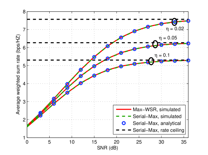
Figure 2: Weighted sum rate performances of the Max-WSR and Serial-Max methods, where $w=0.7$, $N=3$ and $\eta=0.02,0.05,0.1$.

In Fig. 3, we illustrate the average weighted sum rate of the Max-WSR and Serial-Max methods for different numbers of antennas $N=3,4,5$ where the self interference cancelation coefficient is $\eta=0.02$. It can be observed that, for different numbers of antennas, the Serial-Max algorithm achieves almost the same average weighted sum rate as the Max-WSR one across all SNR region. We can also find from this figure that the average weighted sum rate increases with the number of antennas.

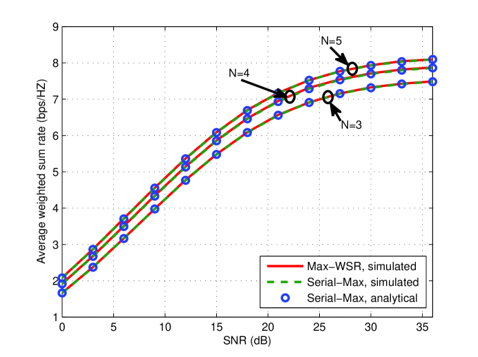
Figure 3: Weighted sum rate performances of the Max-WSR and Serial-Max methods, where $w=0.7$, $\eta=0.02$ and $N=3,4,5$.

V-B Average Weighted Sum SER

The following simulations of weighted sum SER performance are conducted with BPSK modulation. In Fig. 4, the weighted sum SER performance of the Serial-Max method is provided for different $\eta=0,0.05,0.1,0.5$, where large $\eta$ means severe self interference whereas small $\eta$ means slight self interference level. Especially, $\eta=0$ means perfect interference cancelation. This figure verifies the weighted sum SER expression given by Proposition 3. Based on the figure, it can be observed that the simulated SER performance for $\eta=0$ tightly matches with the asymptotic one given by (41) at high SNR, while the SER performances for $\eta>0$ are constrained by error floors evaluated by (31) at high SNR. It can also be seen that when the self interference is perfectly canceled, the diversity order of the Serial-Max method is $(N_{A}-1)(N_{B}-1)$. However when the residual self interference exists, the Serial-Max method has a zero diversity order.

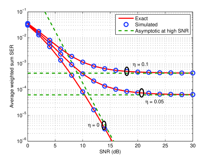
Figure 4: Weighted sum SER performances of the Serial-Max method, where $N=3$ and $\eta=0,0.05,0.1,0.5$.

Fig. 5 shows the average weighted sum SER for different numbers of antennas $N=3,4,5$ where the self interference level $\eta=0.1$ is assumed. It shows that both the Min-WSER and Serial-Max methods are limited by error floors at high SNR due to the residual self interference. As the number of antennas increase, the SER performances of both methods including the error floor are improved. Moreover, the Serial-Max method performs closer to the Min-WSER scheme as $N$ increases.

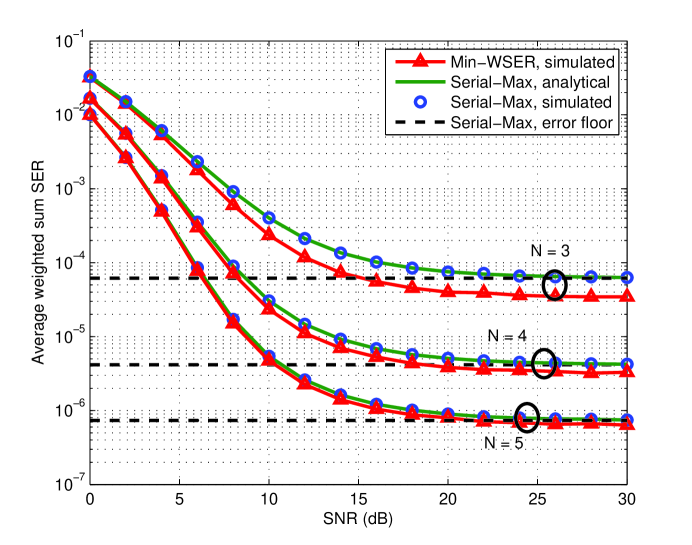
Figure 5: Weighted sum SER performances of the Min-WSER and Serial-Max methods, where $\eta=0.05$ and $N=3,4,5$.

Fig. 6 compares the simulated weighted sum SER performance of the Min-WSER and Serial-Max methods with different number of antennas. Combinations of different SNR and self interference levels ($\lambda_{s}=10,15\rm dB$, $\eta=0.1,0.2$) are provided. It can be observed that the gaps between the Min-WSER and Serial-Max methods are reduced as $N$ increases. It also shows that the SER performance of the Serial-Max method approaches the Min-WSER method when the self interference is large or SNR is small. This is because in these cases these two factors dominate the SER performances of both methods.

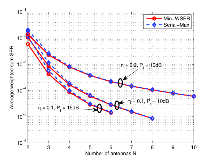
Figure 6: Simulated weighted sum SER performances of the Min-WSER and Serial-Max methods, where $\eta=0.1,0.2$ and $P_{t}=10,15\rm dB$.

V-C Computational complexity

To compare the computational complexity of the optimal and Serial-Max methods, the number of required floating-point operations (flops) are presented in Fig. 7. It is clear that the optimal method has a high complexity due to the brute-force search operation, while the Serial-Max method can provide significant a complexity reduction, especially when the number of antennas is large.

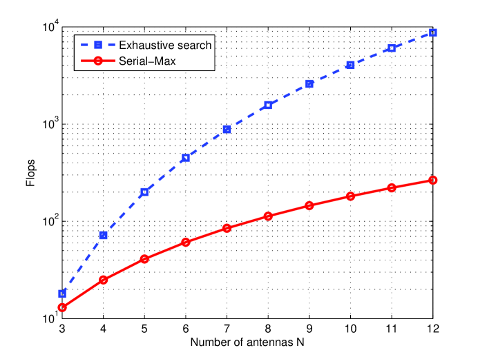
Figure 7: Complexity comparison between the optimal method and the Serial-Max method.

VI Conclusions

In this paper, we have proposed an opportunistic bidirectional link selection approach in FD MIMO systems. The optimal approach based on the “obtainable SINR”, defined as the ratio of the instantaneous SNR and average INR plus one, requires exhaustive search, bearing high complexity. To facilitate the selection process and reduce the computational complexity, a simple Serial-Max method with near optimal performances was proposed. The performance analysis was provide for the Serial-Max method, including the weighted sum rate and SER performances. It was shown that the proposed Serial-Max method approaches the respective weighted sum rate and weighted sum SER performances of the exhaustive search methods when the number of antennas increases.

Appendix A: Proof of Lemma 2

According to the description of the Serial-Max method, the CDF of $\gamma_{AB}$ is expressed as

$${F_{{\gamma_{AB}}}}(x) =\Pr\left({\frac{{\gamma_{s}^{{I_{1}}{J_{1}}}}}{{\gamma_{B}^{RI}+1}}<x}\right)$$ (42)

$$=\Pr\left({\gamma_{s}^{{I_{1}}{J_{1}}}<x\left({\gamma_{B}^{RI}+1}\right)}\right),$$

where $\gamma^{{I_{1}}{J_{1}}}_{s}$ is the largest one of $N_{A}\times N_{B}$ i.i.d. exponential-distributed random variables, and its CDF is given by [23]

$${F_{\gamma_{s}^{{I_{1}}{J_{1}}}}}(x)={\left({1-{e^{-\frac{x}{{{\lambda_{s}}}}}}}\right)^{{N_{A}}{N_{B}}}}.$$ (43)

$\gamma^{RI}_{B}$ follows exponential distribution with average $\lambda_{i}$. Substituting the CDF expression of $\gamma^{{I_{1}}{J_{1}}}_{s}$ and $\gamma^{RI}_{B}$, (42) can be calculated as

$${F_{{\gamma_{AB}}}}(x)=\int\limits_{0}^{\infty}{{{\left[{1-{e^{-\frac{{x\left({\gamma_{B}^{RI}+1}\right)}}{{{\lambda_{s}}}}}}}\right]}^{{N_{A}}{N_{B}}}}\frac{{{e^{-\frac{{\gamma_{B}^{RI}}}{{{\lambda_{i}}}}}}}}{{{\lambda_{i}}}}d\gamma_{B}^{RI}}.$$ (44)

Through some manipulations, we can obtain the CDF of $\gamma_{AB}$.

Appendix B: Proof of Lemma 3

As aforementioned, we have $\gamma_{BA}={\gamma_{s}^{{I_{2}}{J_{2}}}}/({\gamma_{A}^{RI}+1})$, and its CDF expression is

$${F_{{\gamma_{BA}}}}(x) =\Pr\left({\frac{{\gamma_{s}^{{I_{2}}{J_{2}}}}}{{\gamma_{A}^{RI}+1}}<x}\right)$$ (45)

$$=\Pr\left({\gamma_{s}^{{I_{2}}{J_{2}}}<x\left({\gamma_{A}^{RI}+1}\right)}\right).$$

$\gamma_{s}^{{I_{2}}{J_{2}}}$ is the maximum order statistic in the pruned matrix ${\bf\Gamma}_{s}^{\prime}$ consisting of $(N_{A}-1)\times(N_{B}-1)$ random variables following the exponential distribution. Since ${\bf\Gamma}_{s}^{\prime}$ is obtained by removing the maximum element and other $N_{A}+N_{B}-2$ elements from ${\bf\Gamma}_{s}$, $\gamma_{s}^{{I_{2}}{J_{2}}}$ could possibly be one of any $({N_{A}N_{B}}-k)$-th order statistic of ${\bf\Gamma}_{s}$, $k=\{1,2...,N_{A}+N_{B}-1\}$. As a result, the CDF of ${\gamma_{s}^{{I_{2}}{J_{2}}}}$ is given by

$${F_{\gamma_{s}^{{I_{2}}{J_{2}}}}}(x)=\sum\limits_{k=1}^{N_{A}+N_{B}-1}{{p_{k}}{F_{\gamma}^{({{N_{A}N_{B}}}-k)}}(x)},$$ (46)

where $p_{k}$ is the probability that ${\gamma_{s}^{{I_{2}}{J_{2}}}}$ is the $({N_{A}N_{B}}-k)$-th order statistic in ${\bf\Gamma}_{s}$, and ${F_{\gamma}^{({{N_{A}N_{B}}}-k)}}(x)$ represents the CDF of the $({N_{A}N_{B}}-k)$-th order statistic among ${N_{A}N_{B}}$ variables.

For $n$ i.i.d. variables, each with CDF $F(x)$, the CDF of the $r$-th largest order statistic can be written as

$${F^{(r)}}(x)=\sum\limits_{i=r}^{n}{{\binom{n}{i}}{F^{i}}(x){{\left[{1-F(x)}\right]}^{n-i}}}.$$ (47)

Here, they are all exponential variables with average $\lambda_{s}$. Then, the CDF of the $({N_{A}N_{B}}-k)$-th order statistic can be expressed as

$$F_{\gamma}^{({{N_{A}N_{B}}}-k)}(x)= \sum\limits_{l={{N_{A}N_{B}}}-k}^{{{N_{A}N_{B}}}}{\binom{{N_{A}N_{B}}}{l}{{\left({1-{e^{-\frac{x}{{\bar{\gamma}}}}}}\right)}^{l}}{e^{-\frac{{{{N_{A}N_{B}}}-l}}{{\bar{\gamma}}}x}}}$$ (48)

$$= \sum\limits_{l={{N_{A}N_{B}}}-k}^{{{N_{A}N_{B}}}}\hskip 2.84526pt\sum\limits_{m=0}^{l}\binom{{N_{A}N_{B}}}{l}\binom{l}{m}{{(-1)}^{m}}e^{-\frac{{{{N_{A}N_{B}}}-l+m}}{{\bar{\gamma}}}x}.$$

On the other hand, if ${\gamma_{s}^{{I_{2}}{J_{2}}}}$ is the $({N_{A}N_{B}}-k)$-th order statistic in ${\bf\Gamma}_{s}$, it means that among the $(N_{A}+N_{B}-1)$ elements removed from the matrix ${\bf\Gamma}_{s}$, there are $k$ elements larger than ${\gamma_{s}^{{I_{2}}{J_{2}}}}$. To satisfy that the largest element of ${\bf\Gamma}_{s}^{\prime}$ is the $(k+1)$ largest element in ${\bf\Gamma}_{s}$, we can first remove the first $k$ largest elements in the matrix ${\bf\Gamma}_{s}$, and then, keeping the $(k+1)$-th largest element unremoved, we remove the other $(N_{A}+N_{B}-1-k)$ elements randomly. Thus, $p_{k}$ is calculated as

$$p_{k}=\frac{\binom{{N_{A}N_{B}}-k-1}{N_{A}+N_{B}-k-1}}{\binom{{N_{A}N_{B}}-1}{N_{A}+N_{B}-2}},$$ (49)

where the numerator implies that when we remove $(N_{A}+N_{B}-1-k)$ elements randomly from $({N_{A}N_{B}}-k-1)$ elements, there are $\binom{{N_{A}N_{B}}-k-1}{N_{A}+N_{B}-k-1}$ possibilities, while the denominator means that when we remove $(N_{A}+N_{B}-2)$ elements (besides ${\gamma_{s}^{{I_{1}}{J_{1}}}}$, the largest one of ${\bf\Gamma}_{s}$) randomly from $({N_{A}N_{B}}-1)$ elements, there are $\binom{{N_{A}N_{B}}-1}{N_{A}+N_{B}-2}$ possibilities.

Finally, substituting (48) and (49) into (46), the CDF expression of ${\gamma_{s}^{{I_{2}}{J_{2}}}}$ can be obtained as

$${F_{\gamma_{s}^{{I_{2}}{J_{2}}}}}(x)=\sum\limits_{k=1}^{{N_{A}}+{N_{B}}-1}{\sum\limits_{l={N_{A}}{N_{B}}-k}^{{N_{A}}{N_{B}}}{\sum\limits_{m=0}^{l}{{{\left({-1}\right)}^{m}}{\mu_{k,l,m}}}{e^{-\frac{{{N_{A}}{N_{B}}-l+m}}{{\lambda}}x}}}},$$ (50)

where $\mu_{k,l,m}$ is expressed as

$$\mu_{k,l,m}=\frac{\binom{{N_{A}N_{B}}-k-1}{N_{A}+N_{B}-k-1}\binom{{N_{A}N_{B}}}{l}\binom{l}{m}}{\binom{{N_{A}N_{B}}-1}{N_{A}+N_{B}-2}}.$$ (51)

Then, substituting (50) into (45) and combining the CDF of $\gamma_{A}^{RI}$ we have

$${F_{{\gamma_{BA}}}}(x)=\int\limits_{0}^{\infty}{\sum\limits_{k=1}^{{N_{A}}+{N_{B}}-1}{\sum\limits_{l={N_{A}}{N_{B}}-k}^{{N_{A}}{N_{B}}}{\sum\limits_{m=0}^{l}{{{\left({-1}\right)}^{m}}{u_{k,l,m}}}{e^{-\frac{{{N_{A}}{N_{B}}-l+m}}{{{\lambda_{i}}}}x\left({\gamma_{A}^{RI}+1}\right)}}}}\frac{{{e^{-\frac{{\gamma_{A}^{RI}}}{{{\lambda_{i}}}}}}}}{{{\lambda_{i}}}}d\gamma_{A}^{RI}}.$$ (52)

Through some manipulations, Lemma 3 can be obtained.

Appendix C: Proof of Proposition 2

Combining the CDF expression of $\gamma_{AB}$ in (13) and (16), we can obtain

$${{\bar{R}}_{AB}} =\frac{1}{{\ln 2}}\sum\limits_{k=1}^{{N_{A}}{N_{B}}}{{{\left({-1}\right)}^{k+1}}\binom{N_{A}N_{B}}{k}\int\limits_{0}^{\infty}{\frac{{{e^{-\frac{k}{{{\lambda_{s}}}}x}}}}{{\left({k\eta x+1}\right)\left({1+x}\right)}}}dx}$$ (53)

$$=\frac{1}{{\ln 2}}\sum\limits_{k=1}^{{N_{A}}{N_{B}}}{{{\left({-1}\right)}^{k+1}}\binom{N_{A}N_{B}}{k}\int\limits_{0}^{\infty}{\frac{1}{{1-k\eta}}\left[{\frac{{{e^{-\frac{k}{{{\lambda_{s}}}}x}}}}{{\left({1+x}\right)}}-\frac{{k\eta{e^{-\frac{k}{{{\lambda_{s}}}}x}}}}{{k\eta x+1}}}\right]dx}}.$$

Using the integral ${{\rm{E}}_{1}}\left(x\right)={e^{-x}}\int_{0}^{\infty}{\frac{{{e^{-t}}}}{{t+x}}dt}$ [22], (53) can be given by

$${{\bar{R}}_{AB}}=\frac{1}{{\ln 2}}\sum\limits_{k=1}^{{N_{A}}{N_{B}}}{\frac{{{{\left({-1}\right)}^{k}}\binom{N_{A}N_{B}}{k}}}{{1-k\eta}}\left[{{e^{\frac{1}{{\eta{\lambda_{s}}}}}}{{\rm{E}}_{1}}\left({\frac{1}{{\eta{\lambda_{s}}}}}\right)-{e^{\frac{k}{{{\lambda_{s}}}}}}{{\rm{E}}_{1}}\left({\frac{k}{{{\lambda_{s}}}}}\right)}\right]}$$ (54)

On the other hand, the CDF of ${\gamma_{BA}}$ in (14) can be rewritten as

$${F_{\gamma_{BA}}}(x)=1-\sum\limits_{k=1}^{N_{A}+N_{B}-1}{\left({{f_{1}}+{f_{2}}}\right)},$$ (55)

where

$${f_{1}}=\sum\limits_{l={N_{A}}{N_{B}}-k}^{{N_{A}}{N_{B}}-1}{\sum\limits_{m=0}^{l}{{{\left({-1}\right)}^{m+1}}{\mu_{k,l,m}}\frac{{e^{-\frac{{{N_{A}}{N_{B}}-l+m}}{{{\lambda_{s}}}}x}}}{{\left({{N_{A}}{N_{B}}-l+m}\right)\eta x+1}}}},$$ (56)

and

$${f_{2}}=\sum\limits_{m=1}^{{N_{A}}{N_{B}}}{{{\left({-1}\right)}^{m+1}}{\mu_{k,{N_{A}}{N_{B}},m}}\frac{{{e^{-\frac{m}{{{\lambda_{s}}}}x}}}}{{m\eta x+1}}}.$$ (57)

Then, substituting (55)–(57) into (16), we have

$${{\bar{R}}_{BA}}=\frac{1}{{\ln 2}}\sum\limits_{k=1}^{N_{A}+N_{B}-1}{\left({\int\limits_{0}^{\infty}{\frac{{{f_{1}}+{f_{2}}}}{{1+x}}dx}}\right)}.$$ (58)

After some manipulations, the average rate $\bar{R}_{BA}$ in (19) can be obtained. Finally, combining the expression of $\bar{R}_{AB}$ and $\bar{R}_{BA}$, Proposition 2 can be proved.

Appendix D: Proof of Proposition 3

Firstly, substituting the CDF of $\gamma_{AB}$ in (13) into (23), we have

$${\overline{SER}_{AB}}=\frac{1}{2}-\frac{{\alpha\sqrt{\beta}}}{{2\sqrt{2\pi}}}\sum\limits_{k=1}^{{N_{A}}{N_{B}}}{{{(-1)}^{k+1}}\binom{N_{A}N_{B}}{k}\int\limits_{0}^{\infty}{\frac{{{e^{-\left({\frac{\beta}{2}+\frac{k}{{{\lambda_{s}}}}}\right)x}}}}{{\left({k\eta x+1}\right)\sqrt{x}}}dx}}.$$ (59)

Applying Integration by substitution, the integral part is rewritten as

$$\int\limits_{0}^{\infty}{\frac{{{e^{-\left({\frac{\beta}{2}+\frac{k}{{{\lambda_{s}}}}}\right)x}}}}{{\left({k\eta x+1}\right)\sqrt{x}}}dx}\mathop{=}\limits^{t=\sqrt{x}}\int\limits_{0}^{\infty}{\frac{{2{e^{-\left({\frac{\beta}{2}+\frac{k}{{{\lambda_{s}}}}}\right){t^{2}}}}}}{{\left({k\eta{t^{2}}+1}\right)t}}dt}.$$ (60)

Using the integral $\int_{0}^{\infty}{\frac{{{e^{-{a^{2}}{x^{2}}}}}}{{{x^{2}}+{b^{2}}}}dx}=Q\left({\sqrt{2}ab}\right)\frac{\pi}{b}{e^{{a^{2}}{b^{2}}}}$ [28], (60) can be calculated as

$$\int\limits_{0}^{\infty}{\frac{{{e^{-\left({\frac{\beta}{2}+\frac{k}{{{\lambda_{s}}}}}\right)x}}}}{{\left({k\eta x+1}\right)\sqrt{x}}}dx}=\frac{{2\pi}}{{\sqrt{k\eta}}}Q\left({\sqrt{\frac{2}{{\eta{\lambda_{s}}}}+\frac{\beta}{{k\eta}}}}\right){e^{\frac{1}{{\eta{\lambda_{s}}}}+\frac{\beta}{{2k\eta}}}}.$$ (61)

Substituting (61) into (59), and after some manipulation, (27) can be obtained.

Then, the average SER of $\gamma_{BA}$ in (28) can be obtained by substituting (14) into (23) and through the similar manipulations. Finally, combining the two average SER expressions, Proposition 3 can be proved.

References

• [1] J. Choi, M. Jain, K. Srinivasan, P. Levis, and S. Katti, “Achieving single channel, full duplex wireless communication,” in Proc. of MobiCom ACM, New York, NY, USA, Sep. 2010.
• [2] E. Everett, M. Duarte, C. Dick, and A. Sabharwal, “Empowering full- duplex wireless communication by exploiting directional diversity,” in Proc. of Asilomar Conf. Signals, Syst., Comput., pp. 2002–2006, Nov. 2011.
• [3] M. Duarte, C. Dick, and A. Sabharwal, “Experiment-driven characterization of full-duplex wireless systems,” IEEE Trans. Wireless Commun., vol. 11, no. 12, pp. 4296–4307, 2012.
• [4] T. Riihonen, S. Werner, and R. Wichman, “Residual self-interference in full-duplex MIMO relays after null-space projection and cancellation,” in Proc. of Asilomar Conf. Signals, Syst., Comput., pp. 653–657, Nov. 2010.
• [5] B. Chun and Y. H. Lee, “A spatial self-interference nullification method for full duplex amplify-and-forward MIMO relays,” in Proc. of WCNC IEEE, Apr. 2010.
• [6] B. Radunovic, D. Gunawardena, P. Key, A. P. N. Singh, V. Balan, and G. Dejean, “Rethinking indoor wireless: Low power, low frequency, full duplex,” Microsoft Res., Microsoft Corp., Redmond, WA, USA, Tech. Rep., 2009
• [7] D. Senaratne and C. Tellambura, “Beamforming for space division duplexing,” in Proc. of ICC IEEE, Jun. 2011.
• [8] B. P. Day, A. R. Margetts, D. W. Bliss, and P. Schniter, “Full-duplex bidirectional MIMO: Achievable rates under limited dynamic range,” IEEE Trans. Signal Process., vol. 60, no. 7, pp. 3702–3713, Jul. 2012.
• [9] M. Jain, J. I. Choi, T. M. Kim, D. Bharadia, S. Seth, K. Srinivasan, P. Levis, S. Katti, and P. Sinha, “Practival, real-time, full duplex wireless,” in Proc. of MobiCom ACM, Las Vegas, Nevada, USA, Sep. 2011.
• [10] M. Duarte and A. Sabharwal, “Full-duplex wireless communications using off-the-shelf radios: Feasibility and first results,” in Proc. of Asilomar Conf. Signals, Syst., Comput., Pacific Grove, CA, pp. 1558–1562, Nov. 2010.
• [11] H. Ju, X. Shang, H. Poor, and D. Hong, “Bi-directional use of spatial resources and effects of spatial correlation,” IEEE Trans. Wireless Commun., vol. 10, pp. 3368–3379, Oct. 2011.
• [12] D. Kim, H. Ju, S. Park, and D. Hong, “Effects of channel estimation error on full-euplex two-way networks,” IEEE Trans. Veh. Technol., vol. 62, no. 9, pp. 4666–4672, Nov. 2013.
• [13] M. Zhou, H. Cui, L. Song, and B. Jiao, “Transmit-receive antenna pair selection in full duplex systems,” IEEE Wireless Commun. Lett., vol. 3, no. 1, pp. 34-37, Feb. 2014.
• [14] W. Cheng, X. Zhang, and H. Zhang, “QoS driven power allocation over full-duplex wireless links,” in Proc. of ICC IEEE 2012, Jun. 2012.
• [15] W. Cheng, X. Zhang, and H. Zhang, “Optimal dynamic power control for full-duplex bidirectional-channel based wireless networks,” in Proc. of InfoCom IEEE, pp. 3120–3128, Apr. 2013.
• [16] A. Sabharwal, P. Schniter, D. Guo, D. Bliss, S. Rangarajan, R. Wichman, “In-band Full-duplex Wireless: Challenges and Opportunities,” to appear in IEEE J. Sel. Areas Commun., 2014.
• [17] E. Everett, A. Sahai, and A. Sabharwal, “Passive Self-Interference Suppression for Full-Duplex Infrastructure Nodes,” IEEE Trans. Wireless Commun., vol. 13, no. 2, pp. 680–694, Jun. 2013.
• [18] B. P. Day, A. R. Margetts, D. W. Bliss, and P. Schniter,“Full-duplex MIMO relaying: Achievable rates under limited dynamic range,” IEEE J. Sel. Areas Commun., vol. 30, no. 8, pp. 1541–1553, Sep. 2012.
• [19] T.M. Kim and A. Paulraj, “Outage probability of amplify-and-forward cooperation with full duplex relay,” in Proc. of WCNC IEEE, pp. 75–79, Apr. 2012.
• [20] T.K. Baranwal, D.S. Michalopoulos, and R. Schober, “Outage analysis of multihop full duplex relaying,” IEEE Commun. Lett., vol. 17, pp. 63–66, Jan. 2013.
• [21] I. Krikidis, H. Suraweera, P. Smith, and C. Yuen, “Full-duplex relay selection for amplify-and-forward cooperative networks,” IEEE Trans. Wireless Commun., vol. 11, no. 12, pp. 4381–4393, Dec. 2012.
• [22] M. Abramowitz and I. A. Stegun, Handbook of mathematical functions with formulas, graphs, and mathematical tables, 9th ed. NewYork: Dover, 1970.
• [23] H. A. David, Order Statistics. Hoboken, NJ: Wiley, 1970.
• [24] D. Bharadia, E. McMilin, and S. Katti, “Full duplex radios,” in Proceedings of the ACM SIGCOMM, 2013.
• [25] Y. Li, R. H. Y. Louie, and B. Vucetic, “Relay selection with network coding in two-way relay channels,” IEEE Trans. Veh. Technol., vol. 59, no. 9, pp. 4489–4499, Nov. 2010.
• [26] Z. Wang and G. B. Giannakis, “A simple and general parameterization quantifying performance in fading channels,” IEEE Trans. Commun., vol. 51, no. 8, pp. 1389–1398, Aug. 2003.
• [27] Yi Jiang and Varanasi, M.K, “The RF-chain limited mimo system- part I: optimum diversity multiplexing tradeoff,” IEEE Trans. Wireless Commun., vol.8, no. 10, pp. 5238–5246, Oct. 2009.
• [28] I. S. Gradshteyn and I. M. Ryzhik, Table of integals, series, and products, 5th Edition, Academic Press, 1994