Optimal control in Markov decision processes via distributed optimization

Abstract

Optimal control synthesis in stochastic systems with respect to quantitative temporal logic constraints can be formulated as linear programming problems. However, centralized synthesis algorithms do not scale to many practical systems. To tackle this issue, we propose a decomposition-based distributed synthesis algorithm. By decomposing a large-scale stochastic system modeled as a Markov decision process into a collection of interacting sub-systems, the original control problem is formulated as a linear programming problem with a sparse constraint matrix, which can be solved through distributed optimization methods. Additionally, we propose a decomposition algorithm which automatically exploits, if exists, the modular structure in a given large-scale system. We illustrate the proposed methods through robotic motion planning examples.

I Introduction

For many systems, temporal logic formulas are used to describe desirable system properties such as safety, stability, and liveness [1]. Given a stochastic system modeled as a Markov decision process (MDP), the synthesis problem is to find a policy that achieves optimal performance under a given quantitative criterion regarding given temporal logic formulas. For instance, the objective may be to find a policy that maximizes the probability of satisfying a given temporal logic formula. In such a problem, we need to keep track of the evolution of state variables that capture system dynamics as well as predicate variables that encode properties associated with the temporal logic constraints [2, 3]. As the number of states grows exponentially in the number of variables, we often encounter large MDPs, for which the synthesis problems are impractical to solve with centralized methods. The insight for control synthesis of large-scale systems is to exploit the modular structure in a system so that we can solve the original problem by solving a set of small subproblems.

In literature, distributed control synthesis methods are proposed in the pioneering work for MDPs with discounted rewards [4, 5]. The authors formulate a two-stage distributed reinforcement learning method: The first stage constructs and solves an abstract problem derived from the original one, and the second stage iteratively computes parameters for local problems until the collection of local problems’ solutions converge to one that solves the original problem. Recently, alternating direction method of multipliers (ADMM) is combined with a sub-gradient method into planning for average-reward problems in large MDPs in [6]. However, the method in [6] applies only when some special conditions are satisfied on the costs and transition kernels. Alternatively, hierarchical reinforcement learning introduces action-aggregation and action-hierarchies to address the planning problems with large MDPs [7]. In action-aggregation, a micro-action is a local policy for a subset of states and the global optimal policy maps histories of states into micro-actions. However, it is not always clear how to define the action hierarchies and how the choice of hierarchies affects the optimality in the global policy. Additionally, the aforementioned methods are in general difficult to implement and cannot handle temporal logic specifications.

For synthesis problems in MDPs with quantitative temporal logic constraints, centralized methods and tools [3, 8] are developed and applied to control design of stochastic systems and robotic motion planning [9, 10, 11]. Since centralized algorithms are based on either value iteration or linear programming, they inevitably hit the barrier of scalability and are not viable for large MDPs.

In this paper, we develop a distributed optimization method for large MDPs subject to temporal logic contraints. We first introduce a decomposition method for large MDPs and prove a property in such a decomposition that supports the application of the proposed distributed optimization. For a subclass of MDPs whose graph structures are Planar graphs, we introduce an efficient decomposition algorithm that exploits the modular structure for the underlying MDP caused by loose coupling between subsets of states and its constituting components. Then, given a decomposition of the original system, we employ a distributed optimization method called block splitting algorithm [12] to solve the planning problem with respect to discounted-reward objectives in large MDPs and average-reward objectives in large ergodic MDPs. Comparing to two-stage methods in [5, 6, 13], our method concurrently solves the set of sub-problems and penalizes solutions’ mismatches in one step during each iteration, and is easy to implement. Since the distributed control synthesis is independent from the way how a large MDP is decomposed, any decomposition method can be used. Lastly, we extend the method to solve the synthesis problems for MDPs with two classes of quantative temporal logic objectives. Through case studies we investigate the performance and effectiveness of the proposed method.

II Preliminaries

Let $\Sigma$ be a finite set. Let $\Sigma^{\ast},\Sigma^{\omega}$ be the set of finite and infinite words over $\Sigma$. $\mathsf{card}(\Sigma)$ is the cardinality of the set $\Sigma$. A probability distribution on a finite set $S$ is a function $D:S\rightarrow[0,1]$ such that $\sum_{s\in S}D(s)=1$. The support of $D$ is the set $\mathsf{Supp}(D)=\{s\in S\mid D(s)>0\}$. The set of probability distributions on a finite set $S$ is denoted $\mathcal{D}(S)$.

Markov decision process: A Markov decision process (MDP) $M=\langle S,A,u_{0},P\rangle$ consists of a finite set $S$ of states, a finite set $A$ of actions, an initial distribution $u_{0}\in\mathcal{D}(S)$ of states, and a transition probability function $P:S\times A\rightarrow\mathcal{D}(S)$ that for a state $s\in S$ and an action $a\in A$ gives the probability $P(s,a)(s^{\prime})$ of the next state $s^{\prime}$. Given an MDP $M$ we define the set of actions enabled at state $s$ as $A(s)=\{a\in A\mid\exists s^{\prime}\in S,P(s,a)(s^{\prime})>0\}$. The cardinality of the set $\{(s,a)\mid s\in S,a\in A(s)\}$ is the number of state-action pairs in the MDP.

Policies: A path is an infinite sequence $s_{0}s_{1}\ldots$ of states such that for all $i\geq 0$, there exists $a\in A$, $s_{i+1}\in\mathsf{Supp}(P(s_{i},a))$. A policy is a function $f:S^{\ast}\rightarrow\mathcal{D}(A)$ that, given a finite state sequence representing the history, chooses a probability distribution over the set $A$ of actions. Policy $f$ is memoryless if it only depends on the current state, i.e., $f:S\rightarrow\mathcal{D}(A)$. Once a policy $f$ is chosen, an MDP $M$ is reduced to a Markov chain, denoted $M^{f}$. We denote by $X_{i}$ and $\theta_{i}$ the random variables for the $i$-th state and the $i$-th action in this chain $M^{f}$. Given a policy $f$, for a measurable function $\phi$ that maps paths into reals, let $E_{u_{0}}^{f}[\phi]$ (resp. $E_{s}^{f}[\phi]$) be the expected value of $\phi$ when the policy $f$ is used given $u_{0}$ being the initial distribution of states (resp. $s$ being the initial state).

Rewards and objectives: Given an MDP $M$, a reward function $R:S\times A\rightarrow\mathbb{R}$ and a policy $f$, let $\gamma$ be a discounting factor, the discounted-reward value is defined as $\mathsf{Val}_{\gamma}^{f}(u_{0})=\mathsf{Val}_{\gamma}^{f}(s)\cdot u_{0}(s)$ where $\mathsf{Val}_{\gamma}^{f}(s)=E^{f}_{s}(\sum_{n=0}^{\infty}\gamma^{n}R(X_{n},\theta_{n}))$; the average-reward value is defined as $\mathsf{Val}^{f}(u_{0})=\mathsf{Val}^{f}(s)\cdot u_{0}(s)$ where $\mathsf{Val}^{f}(s)=\lim_{n\rightarrow\infty}\frac{1}{n}E_{s}^{f}\left[\sum_{k=0}^{n}R(X_{k},A_{k})\right]$. A discounted-reward (resp. an average-reward) problem is, for a given initial state distribution, to obtain a policy that maximizes the discounted-reward value (resp. average-reward value). For discounted-reward (average-reward) problems, the optimal value can be attained by memoryless policies [14].

A solution to the discounted-reward problem can be found by solving the linear programming (LP) problem:

$$\max_{x\in\mathbb{R}^{m}_{+}}\sum_{s\in S}\sum_{a\in A(v)}x(s,a)\cdot R(s,a)$$ (1a)

subject to (1b)

$$\sum_{a\in A(s)}x(s,a)-\gamma\cdot\sum_{s^{\prime}\in S}\sum_{a^{\prime}\in A(s^{\prime})}x(s^{\prime},a^{\prime})\cdot P(s^{\prime},a^{\prime})(s)$$

$$=u_{0}(s),\forall s\in S,$$ (1c)

where $m$ is the total number of state-action pairs in the MDP, $\mathbb{R}^{m}_{+}$ is the non-negative orthant of $\mathbb{R}^{m}$, and variable $x(s,a)$ can be interpreted as the expected discounted time of being in state $s$ and taking action $a$. Once the LP problem in (1) is solved, the optimal policy is obtained as $f(s,a)=\frac{x(s,a)}{\sum_{a^{\prime}\in A(s)}x(s,a^{\prime})}$ and the objective function’s value is the optimal discounted-reward value under policy $f$ given the initial distribution $u_{0}$ of states.

In an ergodic MDP, the average-reward value is a constant regardless of the initial state distribution [15] (see [15] for the definition of ergodicity). We obtain an optimal policy for an average-reward problem by solving the LP problem

$$\max_{x\in\mathbb{R}^{m}_{+}}\sum_{s\in S}\sum_{a\in A(s)}x(s,a)\cdot R(s,a)$$ (2a)

subject to

$$\sum_{a\in A(s)}x(s,a)-\sum_{s^{\prime}\in S}\sum_{a^{\prime}\in A(s^{\prime})}x(s^{\prime},a^{\prime})\cdot P(s^{\prime},a^{\prime})(s)=0,$$

$$\forall s\in S,$$ (2b)

$$\sum_{s\in S}\sum_{a\in A(s)}x(s,a)=1,$$ (2c)

where $x(s,a)$ is understood as the long-run fraction of time that the system is at state $s$ and the action $a$ is taken. Once the LP problem in (2) is solved, the optimal policy is obtained as $f(s,a)=\frac{x(s,a)}{\sum_{a^{\prime}\in A(s)}x(s,a^{\prime})}$. The optimal objective value is the optimal average-reward value and is the same for all states.

Distributed optimization: As a prelude to the distributed synthesis method developed in section IV, now we describe the alternating direction method of multipliers (ADMM) [16] for the generic convex constrained minimization problem $\min_{z\in\mathbf{C}}g(z)$ where function $g$ is closed proper convex and set $\mathbf{C}$ is closed nonempty convex. In iteration $k$ of the ADMM algorithm the following updates are performed:

$$z^{k+1/2} :=\mathbf{prox}_{g}(z^{k}-\tilde{z}^{k}),$$ (3a)

$$z^{k+1} :=\Pi_{\bf C}(z^{k+1/2}+\tilde{z}^{k}),$$ (3b)

$$\tilde{z}^{k+1} :=\tilde{z}^{k}+z^{k+1/2}-z^{k+1},$$ (3c)

where $z^{k+1/2}$ and $\tilde{z}^{k}$ are auxiliary variables, $\Pi_{\bf C}$ is the (Euclidean) projection onto $\bf C$, and $\mathbf{prox}_{g}(v)=\arg\min_{x}\left(g(x)+(\rho/2)\lVert x-v\rVert_{2}^{2}\right)$ is the proximal operator [16] of $g$ with parameter $\rho>0$. The algorithm handles separately the objective function $g$ in (3a) and the constraint set $\bf C$ in (3b). In (3c) the dual update step coordinates these two steps and results in convergence to a solution of the original problem.

Temporal logic: Linear temporal logic (LTL) formulas are defined by: $\phi:=p\mid\neg\phi\mid\phi_{1}\lor\phi_{2}\mid\bigcirc\phi\mid\phi_{1}\mathcal{U}\phi_{2},$ where $p\in\mathcal{AP}$ is an atomic proposition, and $\bigcirc$ and $\mathcal{U}$ are temporal modal operators for “next” and “until”. Additional temporal logic operators are derived from basic ones: $\lozenge\varphi\coloneqq\mathsf{true}\;\mathcal{U}\varphi$ (eventually) and $\square\varphi\coloneqq\neg\lozenge\neg\varphi$. Given an MDP $M$, let $\mathcal{AP}$ be a finite set of atomic propositions, and a function $L:S\rightarrow 2^{\mathcal{AP}}$ be a labeling function that assigns a set of atomic propositions $L(s)\subseteq\mathcal{AP}$ to each state $s\in S$ that are valid at the state $s$. $L$ can be extended to paths in the usual way, i.e., $L(s\rho)=L(s)L(\rho)$ for $s\in S,\rho\in S^{\omega}$. A path $\rho=s_{0}s_{1}\ldots\in S^{\omega}$ satisfies a temporal logic formula $\varphi$ if and only if $L(\rho)$ satisfies $\varphi$. In an MDP $M$, a policy $f$ induces a probability distribution over paths in $S^{\omega}$. The probability of satisfying an LTL formula $\varphi$ is the sum of probabilities of all paths that satisfy $\varphi$ in the induced Markov chain $M^{f}$.

Problem 1

Given an MDP $M$ and an LTL formula $\varphi$, synthesize a policy that optimizes a quantitative performance measure with respect to the formula $\varphi$ in the MDP $M$.

We consider the probability of satisfying a temporal logic formula as one quantitative performance measure. We also consider the expected frequency of satisfying certain recurrent properties specified in an LTL formula.

By formulating a product MDP that incorporates the underlying dynamics of a given MDP and its temporal logic specification, it can be shown that Problem 1 with different quantitative performance measures can be formulated through pre-processing as special cases of discounted-reward and average-reward problems [3, 17]. Thus, in the following, we first introduce decomposition-based distributed synthesis methods for large MDPs with discounted-reward and average-reward criteria. Then, we show the extension for solving MDPs with quantitative temporal logic constraints.

III Decomposition of an MDP

III-A Decomposition and its property

To exploit the modular structure of a given MDP, the initial step is to decompose the state space into small subsets of states, each of which can then be related to a small problem. In this section, we introduce some terminologies in decomposition of MDPs from [5].

Given an MDP $M=\langle S,A,u_{0},P\rangle$, let $\Pi$ be any partition of the state set $S$. That is, $\Pi=\{S_{1},\ldots,S_{N}\}\subseteq 2^{S}$, $\emptyset\notin\Pi$, $S_{i}\cap S_{j}=\emptyset$ when $i\neq j$ and $\bigcup_{i=1}^{N}S_{i}=S$. A set in $\Pi$ is called a region. The periphery of a region $S_{i}$ is a set of states outside $S_{i}$, each of which can be reached with a non-zero probability by taking some action from a state in $S_{i}$. Formally, $\mathsf{Periphery}(S_{i})=\{s^{\prime}\in S\setminus S_{i}\mid\exists(s,a)\in S_{i}\times A,P(s,a)(s^{\prime})>0\}.$

Let $K_{0}=\bigcup_{i=1}^{N}\mathsf{Periphery}(S_{i})$. Given a region $S_{i}\in\Pi$, we call $K_{i}=S_{i}\setminus K_{0}$ the kernel of $S_{i}$. We denote $m_{i}$ the number of state-action pairs restricted to $K_{i}$, for each $i=0,\ldots,N$. That is, $m_{i}$ is the cardinality of the set $\{(s,a)\mid s\in K_{i},a\in A(s)\}$. We call the partition $\{K_{i}\mid 0\leq i\leq N\}$ a decomposition of $M$. The following property of a decomposition is exploited in distributed optimization.

Lemma 1

Given a decomposition $\{K_{i},i=0,1,\ldots,N\}$ obtained from partition $\Pi=\{S_{1},\ldots,S_{N}\}$, for a state $s\in K_{i}$ where $i\neq 0$, if there is a state $s^{\prime}$ and an action $a$ such that $P(s^{\prime},a)(s)\neq 0$, then either $s^{\prime}\in K_{0}$ or $s^{\prime}\in K_{i}$.

Proof:

Suppose $s^{\prime}\notin K_{0}$ and $s^{\prime}\notin K_{i}$, then it must be the case that $s^{\prime}\in K_{j}$ for some $j\neq 0$ and $j\neq i$. Since from state $s^{\prime}\in S_{j}$, after taking action $a$, the probability of reaching $s\in S_{i}$ is non-zero, we can conclude that $s\in\mathsf{Periphery}(S_{j})$, which implies $s\in K_{0}$. The implication contradicts the fact that $s\in K_{i}$ since $K_{0}\cap K_{i}=\emptyset$. Hence, either $s^{\prime}\in K_{i}$ or $s^{\prime}\in K_{0}$. ∎

Example: Consider the MDP in Figure 1, which is taken from [18]. The shaded region shows a partition $\Pi=\{S_{1}=\{s_{4},s_{5},s_{6}\},S_{2}=\{s_{0},s_{1},s_{2},s_{3},s_{7}\}\}$ of the state space. Then, $\mathsf{Periphery}(S_{1})=\{s_{2},s_{7}\}$ and $\mathsf{Periphery}(S_{2})=\{s_{4}\}$. We obtain a decomposition of $M$ as $K_{0}=\cup_{i=1}^{2}\mathsf{Periphery}(S_{i})=\{s_{2},s_{4},s_{7}\}$, $K_{1}=S_{1}\setminus K_{0}=\{s_{5},s_{6}\}$, and $K_{2}=S_{2}\setminus K_{0}=\{s_{0},s_{1},s_{3}\}$. It is observed that state $s_{5}$ can only be reached with non-zero probabilities by actions taken from states $s_{4}$ and $s_{6}$.

Figure 1: Example of an MDP with states $Q=\{s_{i},i=0,\ldots,7\}$, actions $A=\{\alpha,\beta\}$, and transition probability function $P$ as indicated.

III-B A decomposition method for a subclass of MDPs

Various methods are developed to derive a decomposition of an MDP, for example, decompositions based on partitioning the state space of an MDP according to the communicating classes in the induced graph (defined in the following) of that MDP (see a survey in [13]). For the distributed synthesis method developed in this paper, it will be shown later in Section IV that the number of state-action pairs and the number of states in $K_{i}$ are the number of variables and the number of constraints in a sub-problem, respectively. Thus, we prefer a decomposition that meets one simple desirable property: For each $i=0,1,\ldots,N$, the number $m_{i}$ of state-action pairs in $K_{i}$ is small in the sense that the classical linear programming algorithm can efficiently solve an MDP with state-action pairs of this size. Next, we propose a method that generates decompositions which meet the aforementioned desirable property for a subclass of MDPs. For an MDP in this subclass, its induced graph is Planar . It can be shown that MDPs derived from classical gridworld examples, which have many practical applications in robotic motion planning, are in this subclass.

We start by relating an MDP with a directed graph.

Definition 1

The labeled digraph induced from an MDP $M=\langle S,A,u_{0},P\rangle$ is a tuple $G=\langle S,E\rangle$ where $S$ is a set of nodes, and $E\subseteq S\times A\times S$ is a set of labeled edges such that $(s,a,s^{\prime})\in E$ if and only if $P(s,a)(s^{\prime})>0$.

Let $n=\mathsf{card}(S)$ be the total number of nodes in the graph. A partition of states in the MDP gives rise to a partition of nodes in the graph. Given a partition $\Pi$ and a region $S_{i}\in\Pi$, a node is said to be contained in $S_{i}$ if some edge of the region is incident to the node. A node contained in more than one regions is called a boundary node. That is, $s\in S_{i}$ is a boundary node if and only if there exists $(s,a,s^{\prime})\in E$ or $(s^{\prime},a,s)\in E$ with $s^{\prime}\notin S_{i}$. Formally, the boundary nodes of $S_{i}$ are $B_{i}=\mathsf{In}_{i}\cup\mathsf{Out}_{i}$ where $\mathsf{In}_{i}=\{s\in S_{i}\mid\exists j\neq i,s^{\prime}\in S_{j},a\in A(s^{\prime}),\text{ and }(s^{\prime},a,s)\in E\}$ and $\mathsf{Out}_{i}=\{s\in S_{i}\mid\exists s^{\prime}\in S\setminus S_{i},a\in A(s),\text{ and }(s,a,s^{\prime})\in E\}$. We define $B_{0}=\bigcup_{i=1}^{N}B_{i}$. Note that since $\bigcup_{i=1}^{N}\mathsf{In}_{i}=K_{0}$, $K_{0}\subseteq B_{0}$. We use the number of boundary nodes as an upper bound on the size of the set $K_{0}$ of states.

Definition 2

[20] An $r$-division of an $n$-node graph is a partition of nodes into $O(n/r)$ subsets, each of which have $O(r)$ nodes and $O(\sqrt{r})$ boundary nodes.

Reference [20] shows an algorithm that divides a planar graph of $n$ vertices into an $r$-division in $O(n\log n)$ time.

Lemma 2

Given a partition $\Pi$ of an MDP with $n$ states obtained with a $r$-division the induced graph, the number of states in $K_{0}$ is upper bounded by $O(n/\sqrt{r})$ and the number of states in $K_{i}$ is upper bounded by $O(r)$.

Proof:

Since each boundary node is contained in at most three regions and at least one region by the property of an $r$-division [20], the total number of boundary nodes is $O(\sqrt{r}\cdot\frac{n}{r})=O(n/\sqrt{r})$. The number of states in $K_{i}$ is upper bounded by the size of $S_{i}$, which is $O(r)$. ∎

To obtain a decomposition, the user specifies an approximately upper bound on the number of variables for all sub-problems. Then, the algorithm decides whether there is an $r$-division for some $r$ that gives rise to a decomposition that has the desirable property.

Remark 1

Although the decomposition method proposed here is applicable for a subclass of MDPs, the distributed synthesis method developed in this paper does not constrain the way by which a decomposition is obtained. A decomposition may be given or obtained straight-forwardly by exploiting the existing modular structure of the system. Even if a decomposition does not meet the desirable property for the distributed synthesis method, the proposed method still applies as long as each subproblem derived from that decomposition (see Section IV-C) can be solved given the limitation in memory and computational capacities.

IV Distributed synthesis: Discounted-reward and average-reward problems

In this section, we show that under a decomposition, the original LP problem for a discounted-reward or average-reward case can be formulated into one with a sparse constraint matrix. Then, we employ block-splitting algorithm based on ADMM in [12] for solving the LP problem in a distributed manner.

IV-A Discounted-reward case

Given a decomposition $\{K_{i}\mid i=0,1,\ldots,N\}$ of an MDP, let $x_{i}$ be a vector consisting of variables $x(s,a)$ for all $s\in K_{i}$ with all actions enabled from $s$. Let $\iota_{i}:K_{i}\rightarrow\{1,\ldots,\mathsf{card}(K_{i})\}$ be an index function. The constraints in (1c) can be written as: For each $s\in K_{0}$,

$$\sum_{a\in A(s)}x(s,a)=u_{0}(s)+\\ \gamma\cdot\sum_{i=0}^{N}\sum_{s^{\prime}\in K_{i}}\sum_{a^{\prime}\in A(s^{\prime})}x(s^{\prime},a^{\prime})\cdot P(s^{\prime},a^{\prime})(s),$$ (4)

and for each $s\in K_{i}$, $i=1,\ldots,N$,

$$\sum_{a\in A(s)}x(s,a)=u_{0}(s)+\\ \gamma\cdot\big{(}\sum_{s^{\prime}\in K_{0}}\sum_{a^{\prime}\in A(s^{\prime})}x(s^{\prime},a^{\prime})\cdot P(s^{\prime},a^{\prime})(s)\\ +\sum_{s^{\prime}\in K_{i}}\sum_{a^{\prime}\in A(s^{\prime})}x(s^{\prime},a^{\prime})\cdot P(s^{\prime},a^{\prime})(s)\big{)}.$$ (5)

Recall that, in Lemma 1, we have proven that each $s\in K_{i}$ with $i\neq 0$ can only be reached with non-zero probabilities from states in $K_{0}$ and $K_{i}$. As a result, for each state $s$ in $K_{i}$ with $i\neq 0$ and each action $a\in A(s)$, the constraint on variable $x(s,a)$ is only related with variables in $x_{i}$ and $x_{0}$. Let $x=(x_{0},x_{1},\ldots,x_{N})$. We denote the number of variables in $x_{i}$ by $m_{i}$ and the number of states in the set $K_{i}$ by $n_{i}$. Let $m=\sum_{i=0}^{N}m_{i}$. The LP problem in (1) is then

$$\min_{x\in\mathbb{R}^{m}_{+}}\sum_{j=0}^{N}c_{j}^{T}x_{j},\quad\text{subject to }Ax=b,$$ (6)

where $c_{j}^{T}x_{j}=\sum_{s\in K_{j}}\sum_{a\in A(s)}-R(s,a)x(s,a)$,

$$\small A=\begin{bmatrix}A_{00}&A_{01}&A_{02}&\ldots&A_{0N}\\ A_{10}&A_{11}&&&\\ A_{20}&&A_{22}&&\text{\huge 0}\\ \vdots&\text{\huge 0}&&\ddots&\\ A_{N0}&&&&A_{NN}\end{bmatrix},\quad b=\begin{bmatrix}b_{0}\\ b_{1}\\ b_{2}\\ \vdots\\ b_{N}\end{bmatrix},$$

and $b_{i}\in\mathbb{R}^{n_{i}}$ where $b_{i}(k)=u_{0}(s)$ if $\iota_{i}(s)=k$. The transformation from (4) and (5) to (6) is straightforward by rewriting the constraints and we omit the detail.

IV-B Average-reward case

For an ergodic MDP, the constraints in the LP problem of maximizing the average reward, described by (2b), can be rewritten in the way just as how (1c) is rewritten into (4) and (5) for the discounted-reward problem. The difference is that for the average-reward case, we let $\gamma=1$ and replace $u_{0}(s)$ with $0$, for all $s\in S$, in (4) and (5). An additional constraint for the average-reward case is that $\sum_{s\in S}\sum_{a\in A(s)}x(s,a)=1$. Hence, for an average-reward problem in an ergodic MDP, the corresponding LP problem in (2) is formulated as

$$\min_{x\in\mathbb{R}^{m}_{+}}\sum_{j=0}^{N}c_{j}^{T}x_{j},\quad\text{subject to }\begin{bmatrix}\mathbf{1}^{T}\\ A\end{bmatrix}x=\begin{bmatrix}1\\ \bm{0}\end{bmatrix}$$ (7)

where $\mathbf{1}^{T}$ is a row vector of $m$ ones, $c_{j}^{T}x_{j}=\sum_{s\in K_{j}}\sum_{a\in A(s)}-R(s,a)x(s,a)$ and the block-matrix $A$ has the same structure as of that in the discounted case with $\gamma=1$. We can compactly write the constraint in (7) as $A^{\prime}x=b$ where $A^{\prime}$ is a sparse constraint matrix similar in structure to the matrix $A$ in the discounted-reward case.

IV-C Distributed optimization algorithm

We solve the LP problems in (6) and (7) by employing the block splitting algorithm based on ADMM in [12]. We only present the algorithm for the discounted-reward case in (6). The extension to the average-reward case is straight-forward.

First, we introduce new variables $y_{i}$ and let $f_{i}(y_{i})=I_{\{b_{i}\}}(y_{i})$, where for a convex set $C$, $I_{C}$ is a function defined by $I_{C}(x)=0$ for $x\in C$, $I_{C}(x)=\infty$ for $x\notin C$. Then, adding the term $f_{i}(y_{i})$ into the objective function enforces $y_{i}=b_{i}$. Let $g_{i}(x_{i})=c_{i}^{T}x_{i}+I_{\mathbb{R}^{m_{i}}_{+}}(x_{i})$. The term $I_{\mathbb{R}^{m_{i}}_{+}}(x_{i})$ enforces that $x_{i}$ is a non-negative vector. We rewrite the LP problem in (6) as follows.

$$\begin{split}&\min_{x,y}\sum_{i=0}^{N}f_{i}(y_{i})+\sum_{i=0}^{N}g_{i}(x_{i})\\ \text{subject to }&y_{0}=\sum_{i=0}^{N}A_{0i}x_{i}\text{ and for }i=1,\ldots,N,\;\\ &y_{i}=A_{i0}x_{0}+A_{ii}x_{i}.\end{split}$$ (8)

With this formulation, we modify the block splitting algorithm in [12] to solve (8) in a parallel and distributed manner (see the Appendix for the details). The algorithm takes parameters $\rho$, $\epsilon^{rel}$ and $\epsilon^{abs}$: $\rho>0$ is a penalty parameter to ensure the constraints are satisfied, $\epsilon^{rel}>0$ is a relative tolerance and $\epsilon^{abs}>0$ is an absolute tolerance. The choice of $\epsilon^{rel}$ and $\epsilon^{abs}$ depends on the scale of variable values. In synthesis of MDPs, $\epsilon^{rel}$ and $\epsilon^{abs}$ may be chosen in the range of $10^{-2}$ to $10^{-6}$. The algorithm is ensured to converge with any choice of $\rho$ and the value of $\rho$ may affect the convergence rate.

V Extension to quantitative temporal logic constraints

We now extend the distributed control synthesis methods for MDPs with discounted-reward and average-reward criteria to solve Problem 1 in which quantitative temporal logic constraints are enforced.

V-A Maximizing the probability of satisfying an LTL specification

Preliminaries Given an LTL formula $\varphi$ as the system specification, one can always represent it by a deterministic Rabin automaton (DRA) $\mathcal{A}_{\varphi}=\langle Q,2^{\mathcal{AP}},T,I,\mathsf{Acc}\rangle$ where $Q$ is a finite state set, $2^{\mathcal{AP}}$ is the alphabet, $I\in Q$ is the initial state, and $T:Q\times 2^{\mathcal{AP}}\rightarrow Q$ the transition function. The acceptance condition $\mathsf{Acc}$ is a set of tuples $\{(J_{i},H_{i})\in 2^{Q}\times 2^{Q}\mid i=1,\ldots,\ell\}$. The run for an infinite word $w=\sigma_{0}\sigma_{1}\ldots\in(2^{\mathcal{AP}})^{\omega}$ is the infinite sequence of states $q_{0}q_{1}\ldots\in Q^{\omega}$ where $q_{0}=I$ and $q_{i+1}=T(q_{i},\sigma_{i})$ for $i\geq 0$. A run $\rho=q_{0}q_{1}\ldots$ is accepted in $\mathcal{A}_{\varphi}$ if there exists at least one pair $(J_{i},H_{i})\in\mathsf{Acc}$ such that $\mathsf{Inf}(\rho)\cap J_{i}=\emptyset$ and $\mathsf{Inf}(\rho)\cap H_{i}\neq\emptyset$ where $\mathsf{Inf}(\rho)$ is the set of states that appear infinitely often in $\rho$.

Given an MDP $M=\langle S,A,u_{0},P\rangle$ augmented with a set $\mathcal{AP}$ of atomic propositions and a labeling function $L:S\rightarrow 2^{\mathcal{AP}}$, one can compute the product MDP $\mathcal{M}=M\ltimes\mathcal{A}_{\varphi}=\langle V,A,\Delta,v_{0},\mathsf{Acc}\rangle$ with the components defined as follows: $V=S\times Q$ is the set of states. $A$ is the set of actions. The initial probability distribution of states is $\mu_{0}:V\rightarrow[0,1]$ such that given $v=(s,q)$ with $q=T(I,L(s))$, it is that $\mu_{0}(v)=u_{0}(s)$. $\Delta:V\times A\rightarrow\mathcal{D}(V)$ is the transition probability function. Given $v=(s,q)$, $\sigma$, $v^{\prime}=(s^{\prime},q^{\prime})$ and $q^{\prime}=T(q,L(s^{\prime}))$, let $\Delta(v,\sigma)(v^{\prime})=P(s,\sigma)(s^{\prime})$. The Rabin acceptance condition is $\mathsf{Acc}=\{(\hat{J_{i}},\hat{H_{i}})\mid\hat{J_{i}}=S\times J_{i},\hat{H_{i}}=S\times H_{i},i=1,\ldots,\ell\}$.

By construction, a path $\rho=v_{0}v_{1}\ldots\in V^{\omega}$ satisfies the LTL formula $\varphi$ if and only if there exists $i\in\{1,\ldots,\ell\}$, $\mathsf{Inf}(\rho)\cap\hat{J}_{i}=\emptyset$ and $\mathsf{Inf}(\rho)\cap\hat{H}_{i}\neq\emptyset$. To maximize the probability of satisfying $\varphi$, the first step is to compute the set of end components in $\mathcal{M}$, each of which is a pair $(W,f)$ where $W\subseteq V$ is non-empty and $f:W\rightarrow 2^{A}$ is a function such that for any $v\in W$, for any $a\in f(v)$, $\sum_{v^{\prime}\in W}\Delta(v,a)(v^{\prime})=1$ and the induced directed graph $(W,\rightarrow_{f})$ is strongly connected. Here, $v\rightarrow_{f}v^{\prime}$ is an edge in the graph if there exists $a\in f(v)$, $\Delta(v,a)(v^{\prime})>0$. An end component $(W,f)$ is accepting if $W\cap\hat{J_{i}}=\emptyset$ and $W\cap\hat{H_{i}}\neq\emptyset$ for some $i\in\{1,\ldots,\ell\}$.

Let the set of accepting end components (AEC)s in $\mathcal{M}$ be $\mathsf{AEC}(\mathcal{M})$ and the set of accepting end states be $\mathcal{C}=\{v\mid\exists(W,f)\in\mathsf{AEC}(\mathcal{M}),v\in W\}$. Once we enter some state $v\in\mathcal{C}$, we can find an AEC $(W,f)$ such that $v\in W$, and initiate the policy $f$ such that for some $i\in\{1,\ldots,\ell\}$, states in $\hat{J_{i}}$ will be visited a finite number of times and some state in $\hat{H_{i}}$ will be visited infinitely often.

Formulating the LP problem An optimal policy that maximizes the probability of satisfying the specification also maximizes the probability of hitting the set of accepting end states $\mathcal{C}$. Reference [21] develops GPU-based parallel algorithms which significantly speed up the computation of end components for large MDPs. After computing the set of AECs, we formulate the following LP problem to compute the optimal policy using the proposed decomposition and distributed synthesis method for discounted-reward cases.

Given a product MDP $\mathcal{M}=\langle V,A,\Delta,\mu_{0},\mathsf{Acc}\rangle$ and the set $\mathcal{C}$ of accepting end states, the modified product MDP is $\tilde{\mathcal{M}}=\langle(V\setminus\mathcal{C})\cup\{\mathsf{sink}\},A,\tilde{\Delta},\tilde{\mu}_{0},R\rangle$ where $(V\setminus\mathcal{C})\cup\{\mathsf{sink}\}$ is the set of states obtained by grouping states in $\mathcal{C}$ as a single state $\mathsf{sink}$. For all $a\in A$, $\tilde{\Delta}(\mathsf{sink},a)(\mathsf{sink})=1$ and $\tilde{\Delta}(v,a)(\mathsf{sink})=\sum_{v^{\prime}\in\mathcal{C}}\Delta(v,a)(v^{\prime})$. The initial distribution $\tilde{\mu}_{0}$ of states is defined as follows: For $v\in V\setminus\mathcal{C}$, $\tilde{\mu}_{0}(v)=\mu_{0}(v)$, and $\tilde{\mu}_{0}(\mathsf{sink})=\sum_{v\in\mathcal{C}}\mu_{0}(v)$. The reward function $R:\left((V\setminus\mathcal{C})\cup\{\mathsf{sink}\}\right)\times A\rightarrow\mathbb{R}$ is defined such that for all $v$ that is not $\mathsf{sink}$, $R(v,a)=\sum_{v^{\prime}\in(V\setminus\mathcal{C})\cup\{\mathsf{sink}\}}\tilde{\Delta}(v,a)(v^{\prime})\cdot\bm{1}_{\{\mathsf{sink}\}}(v^{\prime})$ where $\bm{1}_{X}(v)$ is the indicator function that outputs $1$ if and only if $v\in X$ and $0$ otherwise. For any action $a\in A(\mathsf{sink})$, $R(\mathsf{sink},a)=0$.

By definition of reward function, the discounted reward with $\gamma=1$ from state $v$ in the modified product MDP $\tilde{\mathcal{M}}$ is the probability of reaching a state in $\mathcal{C}$ from $v$ under policy $f$ in the product MDP $\mathcal{M}$. Hence, with a decomposition of $\mathcal{M}$, the proposed distributed synthesis method for discounted-reward problems can be used to compute the policy that maximizes the probability of satisfying a given LTL specification.

V-B Average reward under Büchi acceptance conditions

Preliminaries Consider a temporal logic formula $\varphi$ that can be expressed as a deterministic Büchi automaton (DBA) $\mathcal{A}_{\varphi}=\langle Q,2^{\mathcal{AP}},T,I,F_{\varphi}\rangle$ where $Q,2^{\mathcal{AP}},T,I$ are defined similar to a DRA and $F_{\varphi}\subseteq Q$ is a set of accepting states. A run $\rho$ is accepted in $\mathcal{A}_{\varphi}$ if and only if $\mathsf{Inf}(\rho)\cap F_{\varphi}\neq\emptyset$. Given an MDP $M=\langle S,A,u_{0},P,\mathcal{AP},L\rangle$ and a DBA $\mathcal{A}_{\varphi}=\langle Q,2^{\mathcal{AP}},T,q_{0},F_{\varphi}\rangle$, the product MDP with Büchi objective is $\mathcal{M}=M\ltimes\mathcal{A}_{\varphi}=\langle V,A,\Delta,\mu_{0},F\rangle$ where components $V,A,\Delta,\mu_{0}$ are obtained similarly as in the product MDP with Rabin objective. The difference is that $F\subseteq S\times F_{\varphi}$ is the set of accepting states. A path $\rho=v_{0}v_{1}\ldots\in V^{\omega}$ satisfies the LTL formula $\varphi$ if and only if $\mathsf{Inf}(\rho)\cap F\neq\emptyset$.

Formulating the LP problem For a product MDP $\mathcal{M}$ with Büchi objective, we aim to synthesize a policy that maximizes the expected frequency of visiting an accepting state in the product MDP $\mathcal{M}=M\ltimes\mathcal{A}_{\varphi}$. This type of objectives ensures some recurrent properties in the temporal logic formula are satisfied as frequently as possible. For example, one such objective can be requiring a mobile robot to maximize the frequency of visiting some critical regions.

This type of objectives can be formulated as an average-reward problem in the following way: Let the reward function $R:V\times A\rightarrow\mathbb{R}$ be defined by $R(v,a)=\sum_{v^{\prime}\in V}\Delta(v,a)(v^{\prime})\cdot\mathbf{1}_{F}(v^{\prime})$. By definition of the reward function, the optimal policy with respect to the average-reward criterion is the one that maximizes the frequency of visiting a state in $F$. If the product MDP is ergodic, we can then solve the resulting average-reward problem by the distributed optimization algorithm with a decomposition of product MDP $\mathcal{M}$.

VI Case studies

We demonstrate the method with three robot motion planning examples. All the experiments were run on a machine with Intel Xeon 4 GHz, 8-core CPU and 64 GB RAM running Linux. The distributed optimization algorithm is implemented in MATLAB. The decomposition and other operations are implemented in Python.

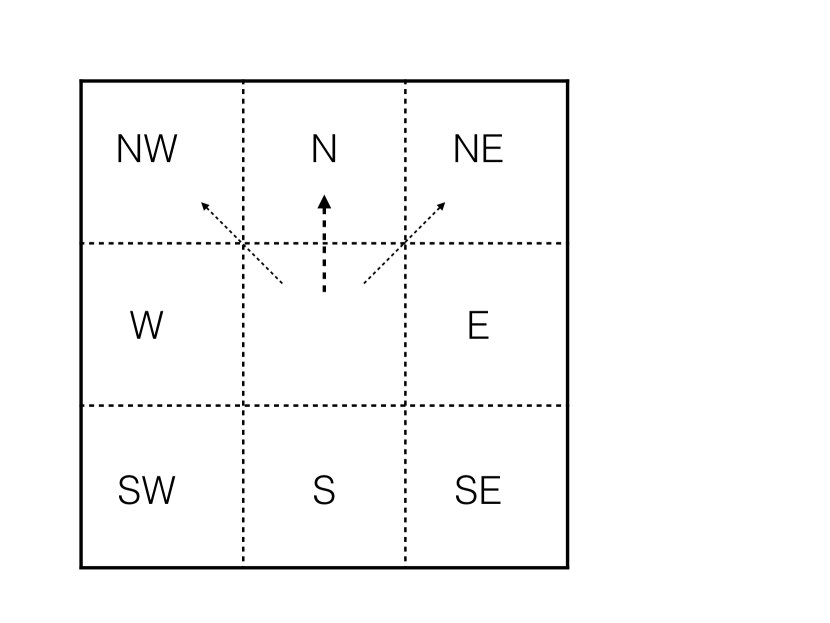
(a)

(b)

Figure 2: (a) A fraction of a $m\times n$ gridworld. The dash arrow represents that if the robot takes action ‘N’, there are non-zero probabilities for it to arrive at NW, N, and NE cells. (b) A $20\times 20$ gridworld. A natural partition of state space using the walls gives rise to $K_{0},K_{1},K_{2},K_{3},K_{4}$ subsets of states. States in $K_{0}$ are enclosed using the squares.

Figure 2(a) shows a fraction of a gridworld. A robot moves in this gridworld with uncertainty in different terrains (‘grass’, ‘sand’, ‘gravel’ and ‘pavement’). In each terrain and for robot’s different action (heading north (‘N’), south (‘S’), west (‘W’) and east (‘E’)), the probability of arriving at the correct cell is $0.9$ for pavement, $0.85$ for grass, $0.8$ for gravel and $0.75$ for sand. With a relatively small probability, the robot will arrive at the cell adjacent to the intended one. Figure 2(b) displays a $20\times 20$ gridworld. The grey area and the boundary are walls. If the robot runs into the wall, it will be bounce back to its original cell. The walls give rise to a natural partition of the state space, as demonstrated in this figure. If no explicit modular structure in the system can be found, one can compute a decomposition using the method in section III-B. In the following example, the wall pattern is the same as in the $20\times 20$ gridworld.

VI-A Discounted-reward case

We select a subset $W$ of cells as “restricted area” and a subset $G$ of cells as “targets”. The reward function is given: For $s\in S$, $S\notin G\cup W$, $R(s,a)=-1$ counts for the amount of time the robot takes action $a$. For $s\in W$, for all $a\in A(s)$, $R(s,a)=-1000$. For $s\in G$, $R(s,a)=100$ for all $a\in A(s)$. Intuitively, this reward function will encourage the robot to reach the target with as fewer expected number of steps as possible, while avoiding running into a cell in the restricted area. We select $\gamma=0.9$.

Case 1: To show the convergence and correctness of the distributed optimization algorithm, we first consider a $100\times 100$ gridworld example that can be solved directly with a centralized algorithm. Since at each cell there are four actions for the robot to pick, the total number of variables is $4\times 8220$ for the $100\times 100$ gridworld (the wall cells are excluded from the set of states). In this gridworld, there is only $1$ target cell. The restricted area include $50$ cells. The resulting LP problem (1) can be solved using CVX, a package for specifying and solving convex programs [22]. The problem is solved in $4.77$ seconds, and the optimal objective value under the optimal policy given by CVX is $10$.

Next, we solve the same problem by decomposing the state space of the MDP along the walls into $25$ regions, each of which is a $20\times 20$ gridworld. This partition of state space yields $75$ states for each $K_{i},i>0$ and $720$ states for $K_{0}$. In which follows, we select $\rho=80,100,200,500,1000$ to show the convergence of the distributed optimization algorithm. Irrespective of the choices for $\rho$, the average time for each iteration is about $0.16$ sec. The solution accuracy relative to CVX is summarized in Table I. The ‘rel. error in objval’ is the relative error in objective value attained, treating the CVX solution as the accurate one, and the infeasibility is the relative primal infeasibility of the solution, measured by $\frac{\lVert Ax^{\ast}-b\rVert_{2}}{1+\lVert b\rVert_{1}}.$ Figure 3 shows the convergence of the optimization algorithm.

TABLE I: Relative resolution accuracy for solving the $100\times 100$ gridworld example with discounted reward (under $\epsilon^{abs}=10^{-5}$, $\epsilon^{rel}=10^{-4}$).

$\rho$	80	100	200	500	1000
Iterations	12001	11014	13868	11866	12733
objval	9.54	9.90	9.89	9.96	9.96
rel. error ($\%$)	4.6	1.0	1.1	0.38	0.38
infeasibility	$2.7\times 10^{-3}$	$2\times 10^{-3}$	$0.885\times 10^{-3}$	$0.45\times 10^{-3}$	$0.23\times 10^{-3}$

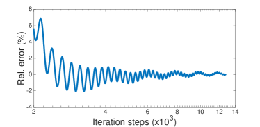
Figure 3: Relative error in the objective value vesus iterations in $100\times 100$ gridworld with discounted reward, under $\rho=1000$. For clarity, we did not draw the relative error for the initial $2000$ steps, which are comparatively large.

Case 2: For a $1000\times 100$ gridworld, the centralized method in CVX fails to produce a solution for this large-scale problem. Thus, we consider to solve it using the decomposition and distributed synthesis method. In this example, we partition the gridworld such that each region has $50\times 50$ cells, which results in $40$ regions. There are $1160$ states in $K_{0}$ and about $2005$ states in each $K_{i}$, for $i=1,\ldots,40$. In this example, we randomly select $40$ cells to be the targets and $40$ cells to be the restricted areas. By choosing $\rho=1000$, $\epsilon^{rel}=10^{-6}$, $\epsilon^{abs}=10^{-6}$, the optimal policy is solved within $25342$ seconds and it takes about $2.6$ seconds for one iteration. The total number of iterations is $9747$. Under the (approximately)-optimal policy obtained by distributed optimization, the objective value is $138.73$. The relative primal infeasibility of the solution is $0.29\times 10^{-4}$. Figure 4(a) shows the convergence of distributed optimization algorithm.

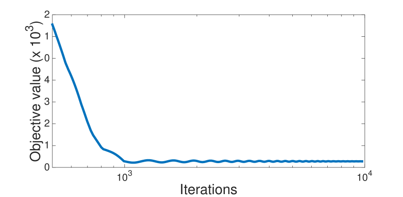
(a)

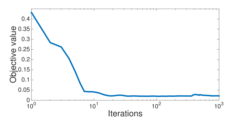
(b)

Figure 4: Objective value vesus iterations in (a) $1000\times 100$ gridworld (the initial $500$ steps are omitted). (b) Objective value vesus iterations in $50\times 50$ gridworld with a Büchi objective. Here we only show the first $1000$ iterations as the objective value converges to the optimal one after $1000$ steps.

VI-B Average-reward case with quantative temporal logic objectives

We consider a $50\times 50$ gridworld with no obstacles and $4$ critical regions labeled “$R_{1}$” , “$R_{2}$”, “$R_{3}$” and “$R_{4}$”. The system is given a temporal logic specification $\varphi\coloneqq\square\lozenge(R_{1}\land\lozenge R_{2})\land\square\lozenge(R_{3}\land\lozenge R_{4})$. That is, the robot has to always eventually visit region $R_{1}$ and then $R_{2}$, and also always eventually visit region $R_{3}$ and then $R_{4}$. The number of states in the corresponding DBA is $14$ after trimming the unreachable states, due to the fact that the robot cannot be at two cells simultaneously. The quantitative objective is to maximize the frequency of visiting all four regions (an accepting state in the DBA). The formulated MDP is ergodic and therefore our method for average-reward problems applies.

For an average-reward case, we need to satisfy the constraint $\mathbf{1}^{T}x=1$ in (7). This constraint leads to slow convergence and policies with large infeasibility measures in distributed optimization. To handle this issue, we approximate average reward with discounted reward [23]: For ergodic MDPs, the discounted accumulated reward, scaled by $1-\gamma$, is approximately the average reward. Further, if $\frac{1}{1-\gamma}$ is large compared to the mixing time [15] of the Markov chain, then the policy that optimizes the discounted accumulated reward with the discounting factor $\gamma$ can achieve an approximately optimal average reward.

Given $\rho=1000$, $\epsilon^{ref}=10^{-5}$ and $\epsilon^{abs}=10^{-5}$, $\gamma=0.98$, the distributed synthesis algorithm terminates in $14284$ iteration steps and the optimal discounted reward is $0.9998$. Scaling by $1-\gamma=0.02$, we obtain the average reward $0.9998\times 0.02=0.02$, which is the approximately optimal value for this average reward under the obtained policy. The convergence result is shown in Figure 4(b) and the infeasibility measure of the obtained solution is $0.016$.

VII Conclusion

For solving large Markov decision process models of stochastic systems with temporal logic specifications, we developed a decomposition algorithm and a distributed synthesis method. This decomposition exploits the modularity in the system structure and deals with sub-problems of smaller sizes. We employed the block splitting algorithm in distributed optimization based on the alternating direction method of multipliers to cope with the difficulty of combining the solutions of sub-problems into a solution to the original problem. Moreover, the formal decomposition-based distributed control synthesis framework established in this paper facilitates the application of other distributed and parallel large-scale optimization algorithms [24] to further improve the rate of convergence and the feasibility of solutions for control synthesis in large MDPs. In the future, we will develop an interface to PRISM toolbox [8] with an implementation of the proposed decomposition and distributed synthesis algorithms.

Appendix A Appendix

At the $k$-th iteration, for $i,j=0,\ldots,N$,

$$\begin{split}y_{i}^{k+1/2}&:=\mathbf{prox}_{f_{i}}(y_{i}^{k}-\tilde{y}_{i}^{k})=b_{i},\\ x_{j}^{k+1/2}&:=\mathbf{prox}_{g_{j}}(x_{j}^{k}-\tilde{x}_{j}^{k})\\ &=\mathbf{proj}_{\mathbb{R}_{+}^{m_{j}}}(x_{j}^{k}-\tilde{x}_{j}^{k}-c_{j}/\rho),\\ (x_{ij}^{k+1/2},y_{ij}^{k+1/2})&:=\mathbf{proj}_{ij}(x_{j}^{k}-\tilde{x}_{ij}^{k},y_{ij}^{k}+\tilde{y}_{i}^{k}),\\ x_{j}^{k+1}&:=\mathbf{avg}(x_{j}^{k+1/2},\{x_{ij}^{k+1/2}\}_{i=0}^{N}),\\ (y_{i}^{k+1},\{y_{ij}^{k+1}\}_{j=0}^{N})&:=\mathbf{exch}(y_{i}^{k+1/2},\{y_{ij}^{k+1/2}\}_{j=0}^{N}),\\ &\text{ if }i=0,\\ (y_{i}^{k+1},\{y_{i0}^{k+1},y_{ii}^{k+1}\})&:=\mathbf{exch}(y_{i}^{k+1/2},\{y_{i0}^{k+1/2},y_{ii}^{k+1/2}\}),\\ &\text{ if }i=1,\ldots,N,\\ \tilde{x}_{j}^{k+1}&:=\tilde{x}_{j}^{k}+x_{j}^{k+1/2}-x_{j}^{k+1},\\ \tilde{y}_{i}^{k+1}&:=\tilde{y}_{i}^{k}+y_{i}^{k+1/2}-y_{i}^{k+1},\\ \tilde{x}_{ij}^{k+1}&:=\tilde{x}_{ij}^{k}+x_{ij}^{k+1/2}-x_{j}^{k+1},\end{split}$$

where $\mathbf{proj}_{R^{m_{i}}_{+}}$ denotes the projection to the nonnegative orthant, $\mathbf{proj}_{ij}$ denotes projection onto $\{(x,y)\mid y=A_{ij}x\}$. $\mathbf{avg}$ is the elementwise averaging ; and $\mathbf{exch}$ is the exchange operator, defined as below. $\mathbf{exch}(c,\{c_{j}\}_{j=1}^{N})$ is given by $y_{ij}:=c_{j}+(c-\sum_{j=1}^{N}c_{j})/(N-1)$ and $y_{i}:=c-(c-\sum_{j=1}^{N}c_{j})/N-1$. The variables can be initialized to $0$ at $k=0$. Note that the computation in each iteration can be parallelized. The iteration terminates when the stopping criterion for the block splitting algorithm is met (See [12] for more details). The solution can be obtained $x^{\ast}=(x_{0}^{k+1/2},\ldots,x_{N}^{k+1/2})$.

References

- [1] Z. Manna and A. Pnueli, The Temporal Logic of Reactive and Concurrent Systems: Specifications. springer, 1992, vol. 1.
- [2] S. Thiébaux, C. Gretton, J. K. Slaney, D. Price, F. Kabanza, and Others, “Decision-Theoretic Planning with non-Markovian Rewards.” Journal of Artificial Intelligence Research, vol. 25, pp. 17–74, 2006.
- [3] C. Baier and J.-P. Katoen, Principles of Model Checking. MIT press Cambridge, 2008.
- [4] H. J. Kushner and C.-H. Chen, “Decomposition of systems governed by markov chains,” IEEE Transactions on Automatic Control, vol. 19, no. 5, pp. 501–507, 1974.
- [5] T. Dean and S.-H. Lin, “Decomposition techniques for planning in stochastic domains,” in Proceedings of the 14th international joint conference on Artificial intelligence-Volume 2. Morgan Kaufmann Publishers Inc., 1995, pp. 1121–1127.
- [6] V. Krishnamurthy, C. Rojas, and B. Wahlberg, “Computing monotone policies for markov decision processes by exploiting sparsity,” in Australian Control Conference, Nov 2013, pp. 1–6.
- [7] A. G. Barto and S. Mahadevan, “Recent advances in hierarchical reinforcement learning,” Discrete Event Dynamic Systems, vol. 13, no. 4, pp. 341–379, 2003.
- [8] M. Kwiatkowska, G. Norman, and D. Parker, “PRISM 4.0: Verification of probabilistic real-time systems,” in Proceedings of International Conference on Computer Aided Verification, ser. LNCS, G. Gopalakrishnan and S. Qadeer, Eds., vol. 6806. Springer, 2011, pp. 585–591.
- [9] X. C. Ding, S. L. Smith, C. Belta, and D. Rus, “MDP optimal control under temporal logic constraints,” in IEEE Conference on Decision and Control and European Control Conference, 2011, pp. 532–538.
- [10] E. M. Wolff, U. Topcu, and R. M. Murray, “Optimal control with weighted average costs and temporal logic specifications.” in Robotics: Science and Systems, 2012.
- [11] M. Lahijanian, S. Andersson, and C. Belta, “Temporal logic motion planning and control with probabilistic satisfaction guarantees,” IEEE Transactions on Robotics, vol. 28, no. 2, pp. 396–409, April 2012.
- [12] N. Parikh and S. Boyd, “Block splitting for distributed optimization,” Mathematical Programming Computation, vol. 6, no. 1, pp. 77–102, Oct. 2013.
- [13] C. Daoui, M. Abbad, and M. Tkiouat, “Exact decomposition approaches for Markov decision processes: A survey,” Advances in Operations Research, vol. 2010, pp. 1–19, 2010.
- [14] D. P. Bertsekas, Dynamic Programming and Optimal Control, Vol. II, 3rd ed. Athena Scientific, 2007.
- [15] M. L. Puterman, Markov Decision Processes: Discrete Stochastic Dynamic Programming. John Wiley & Sons, 2009, vol. 414.
- [16] S. Boyd, N. Parikh, E. Chu, B. Peleato, and J. Eckstein, “Distributed optimization and statistical learning via the alternating direction method of multipliers,” Foundations and Trends in Machine Learning, vol. 3, no. 1, pp. 1–122, 2011.
- [17] T. Brázdil, V. Brozek, K. Chatterjee, V. Forejt, and A. Kucera, “Two views on multiple mean-payoff objectives in markov decision processes,” in Annual IEEE Symposium on Logic in Computer Science, 2011, pp. 33–42.
- [18] C. Baier, M. Größ er, M. Leucker, B. Bollig, and F. Ciesinski, “Controller Synthesis for Probabilistic Systems (Extended Abstract),” in Exploring New Frontiers of Theoretical Informatics, ser. IFIP International Federation for Information Processing, J.-J. Levy, E. Mayr, and J. Mitchell, Eds. Springer US, 2004, vol. 155, pp. 493–506.
- [19] H. J. Kushner and P. Dupuis, Numerical Methods for Stochastic Control Problems in Continuous Time. Springer, 2001, vol. 24.
- [20] G. N. Federickson, “Fast algorithms for shortest paths in planar graphs, with applications,” SIAM Journal on Computing, vol. 16, no. 6, pp. 1004–1022, 1987.
- [21] A. Wijs, J.-P. Katoen, and D. Bošnački, “Gpu-based graph decomposition into strongly connected and maximal end components,” in Computer Aided Verification, ser. Lecture Notes in Computer Science, A. Biere and R. Bloem, Eds. Springer International Publishing, 2014, vol. 8559, pp. 310–326.
- [22] M. Grant and S. Boyd, “CVX: Matlab software for disciplined convex programming, version 2.1,” Mar. 2014.
- [23] S. Kakade, “Optimizing average reward using discounted rewards,” in Computational Learning Theory. Springer, 2001, pp. 605–615.
- [24] G. Scutari, F. Facchinei, L. Lampariello, and P. Song, “Parallel and distributed methods for nonconvex optimization,” in IEEE International Conference on Acoustics, Speech and Signal Processing, May 2014, pp. 840–844.