A Multi-Wavelength Mass Analysis of RCS2 J232727.6-020437, a $\sim 3\times 10^{15}$M_☉ Galaxy Cluster at z=0.7

Abstract

We present an initial study of the mass and evolutionary state of a massive and distant cluster, RCS2 J232727.6-020437. This cluster, at z=0.6986, is the richest cluster discovered in the RCS2 project. The mass measurements presented in this paper are derived from all possible mass proxies: X-ray measurements, weak-lensing shear, strong lensing, Sunyaev Zel’dovich effect decrement, the velocity distribution of cluster member galaxies, and galaxy richness. While each of these observables probe the mass of the cluster at a different radius, they all indicate that RCS2 J232727.6-020437  is among the most massive clusters at this redshift, with an estimated mass of $M_{200}\sim 3\times 10^{15}$${h}_{70}^{-1}$M_☉. In this paper, we demonstrate that the various observables are all reasonably consistent with each other to within their uncertainties. RCS2 J232727.6-020437  appears to be well relaxed – with circular and concentric X-ray isophotes, with a cool core, and no indication of significant substructure in extensive galaxy velocity data.

1. Introduction

High redshift clusters have been successfully identified in dedicated surveys working with a range of cluster-selecting techniques and wavelengths. These include cluster discoveries in deep X-ray observations (e.g., Gioia & Luppino, 1994; Rosati et al., 1998; Romer et al., 2000; Ebeling et al., 2001; Rosati et al., 2004; Mullis et al., 2005; Stanford et al., 2006; Rosati et al., 2009); optical$+$near infrared imaging (e.g., Gladders & Yee, 2005; Stanford et al., 2005; Brodwin et al., 2006; Elston et al., 2006; Wittman et al., 2006; Eisenhardt et al., 2008; Muzzin et al., 2009; Wilson et al., 2009; Papovich et al., 2010; Brodwin et al., 2011; Santos et al., 2011; Gettings et al., 2012; Stanford et al., 2012; Zeimann et al., 2012; Stanford et al., 2014), and detection of the the Sunyaev Zel’dovich (SZ) effect (Staniszewski et al., 2009; Vanderlinde et al., 2010; Williamson et al., 2011; Marriage et al., 2011; Planck Collaboration et al., 2013; Hasselfield et al., 2013; Reichardt et al., 2013; Brodwin et al., 2014; Bleem et al., 2015).

Nevertheless, despite this extensive effort, these surveys resulted in a modest number of high redshift ($z\gtrsim 0.5$) and massive ($M\gtrsim 10^{15}$M_☉) galaxy clusters. This relative paucity of distant massive clusters is a reflection both of the challenges inherent in detecting such clusters and of their intrinsic rarity (e.g., Crocce et al., 2010). Such clusters are the earliest and largest collapsed halos; the observed density of distant massive clusters is thus exquisitely sensitive to several cosmological parameters (e.g., Eke et al., 1996) and indeed the presence of a single cluster in prior cluster surveys has been used to limit cosmological models (e.g., Bahcall & Fan, 1998). Such clusters also offer, at least in principle, the opportunity to test for non-gaussianity on cluster scales if the cosmology is otherwise constrained (e.g., Sartoris et al., 2010).

At $0.6<z<1.0$, the most massive galaxy clusters known to date are CL J1226$+$3332 (Maughan et al., 2004) at $z=0.89$ with mass of $M_{200}=1.38\pm 0.20\times 10^{15}$${h}_{70}^{-1}$M_☉  (Jee & Tyson, 2009), ACT-CL J0102–4915 at $z=0.87$ and with $M_{200}=2.16\pm 0.32\times 10^{15}$${h}_{70}^{-1}$M_☉  (Menanteau et al., 2012), and MACS0744.8$+$3927 at $z=0.698$ with $M(<1.5\rm{Mpc})=2.05\pm 0.57\times 10^{15}$${h}_{70}^{-1}$M_☉  (Applegate et al., 2014). Recently discovered $z>1.0$ galaxy clusters appear to have more moderate masses, e.g., SPT-CL J2106–5844 ($z=1.14$, $M_{200}=1.27\pm 0.21\times 10^{15}$${h}_{70}^{-1}$M_☉; Foley et al. 2011), SPT-CL J2040–4451 ($z=1.48$, $M_{200}=5.8\pm 1.4\times 10^{14}$${h}_{70}^{-1}$M_☉; Bayliss et al. 2014b) and IDCS J1426.5$+$3508 ($z=1.75$, $M_{200}=4.3\pm 1.1\times 10^{14}$${h}_{70}^{-1}$M_☉; Brodwin et al. 2012).

Massive clusters at any redshift are amenable to detailed study with a density of data that less massive systems do not present. The X-ray luminosity of clusters scales as M^1.80 (Pratt et al., 2009), the SZ decrement as M^1.66 (Bonamente et al., 2008), the weak-lensing shear approximately as $M_{200}^{2/3}$, and the galaxy richness in a fixed metric aperture (and hence the available number of cluster galaxy targets for spectroscopic and dynamical studies within a given field of view) scales as M^0.6 (Yee & Ellingson, 2003) at these masses. Similarly it is expected that the most massive clusters dominate the cross-section for cluster-scale strong lensing (Hennawi et al., 2007). Thus the most massive clusters offer a wealth of potentially well-measured observables which can be used, for example, to study the correspondance between different mass proxies; such study is critical to the success of surveys which aim to use the redshift evolution of the cluster mass function as a cosmological probe.

We present here detailed observations of a single massive cluster selected from the Second Red-Sequence Cluster Survey (RCS2; Gilbank et al., 2011). This cluster, RCS2 J232727.6-020437  (hereafter RCS2327), was selected from RCS2  in an early and partial cluster catalog. Its optical properties indicated that it is a very massive cluster, and justified an extensive followup campaign with ground-based and space-based observatories at all wavelengths, from X-ray to radio. Since its discovery, some of the properties of RCS2327  have been reported on in the literature. Gralla et al. (2011) first measured its mass from Sunyaev Zel’dovich array observations and its Einstein radius from strong lens modeling. RCS2327  was rediscovered as the highest significance cluster in the Atacama Cosmology Telescope survey (Hasselfield et al. 2013), and Menanteau et al. (2012) also report on mass estimates from archival optical and X-ray observations.

Although the discovery publication of RCS2327  has been delayed, it was advertised in the past decade in various oral presentations and conferences – in order to motivate more extensive followup effort by the community. Indeed deeper and more detailed observations have been conducted since, and will be the basis of future publications. This paper presents mass estimates from the initial survey and early multi-wavelength followup observations of RCS2327, which collectively indicate that it is an unusually massive high-redshift cluster of galaxies.

This paper is organized as follows. The appearance of the cluster in the RCS2  data and catalogs is discussed in § 2. We describe the various datasets and corresponding analyses (richness and galaxy photometry, dynamics, X-ray, SZ decrement, weak- and strong-lensing) in detail in § 3. We discuss the implications of these observations in § 4 and conclude in § 5.

Throughout the paper we use the conventional notation $M_{200}$ ($M_{500}$, $M_{2500}$) to denote the enclosed mass within a radius $R_{200}$ ($R_{500},R_{2500}$), where the overdensity is 200 (500, 2500) the critical matter density at the cluster redshift. Unless otherwise stated, we used the WMAP 5-year cosmology parameters (Komatsu et al., 2009), with $\Omega_{\Lambda}=0.73$, $\Omega_{m}=0.27$, and $H_{0}=70$ km s^-1 Mpc^-1. In this cosmology, $1\arcsec$ corresponds to 7.24 kpc at the cluster redshift, $z=0.6986$. Magnitudes are reported in the AB system.

2. The Second Red-Sequence Cluster Survey and the Discovery of RCS2327

The Second Red-Sequence Cluster Survey (RCS2) is an imaging program executed using the Megacam facility at CFHT. RCS2 is described in full in Gilbank et al. (2011). In short, images have been acquired in the $g$, $r$, and $z$ filters, with integration times of 4, 8, and 6 minutes respectively, and all with sub-arcsecond seeing conditions via observations in queue mode. The RCS2 data are approximately 1-2 magnitudes deeper than the Sloan Digital Sky Survey imaging (York et al., 2000), with a 5-$\sigma$ point-source limiting magnitudes of 24.4, 24.3, and 22.8 mag in $g$, $r$, and $z$ respectively. The RCS2 survey data comprise 785 unique pointings of the nominally 1 square degree CFHT Megacam camera; the surveyed area is somewhat less than 700 square degrees once data masking and pointing overlaps are accounted for. The cluster and group catalog from RCS2 extend to $z\sim 1.1$, constructed using the techniques described in Gladders & Yee (2005). The $g$-band imaging improves the overall performance at lower redshifts (compared to RCS1; Gladders & Yee 2005), and makes the survey more adept at detecting strong lensing clusters, since lensed sources tend to have blue colors.

RCS2327 was discovered in 2005 in an early and partial version of the RCS2 cluster catalog. An examination of the RCS2 survey images made it clear that it was an unusually massive object. A color image of RCS2327 is shown in Figure 1. The original RCS2 imaging data clearly showed at least one strongly lensed arc, and the indicated cluster photometric redshift was $z\sim 0.7$. A plot of the detection significance versus photometric redshift for clusters from the RCS2 cluster catalog is shown in Figure 2. The RCS2 imaging data are fairly uniform, and so at a given redshift the detection significance is a meaningful quantity that is not strongly affected by data quality from region to region of the survey. At high redshifts RCS2327 is the most significant cluster detected. Furthermore, a cluster of a given richness and compactness (both of which influence detection significance) will be detected as a more significant object at lower redshifts; the fact that RCS2327 is detected with a significance as great as any lower redshift clusters implies that it is likely the most massive cluster in this sample. Even from these basic data and considering the volume probed it is apparent that RCS2327 is a remarkably massive cluster, worthy of significant followup.

The cluster is located at R.A.$=$23:27:27.61 (J2000) and Decl.$=-$02:04:37.2 (J2000); this is the position of the brightest cluster galaxy (BCG) and is coincident with the center of the cluster X-ray emission (see § 3.3 below).

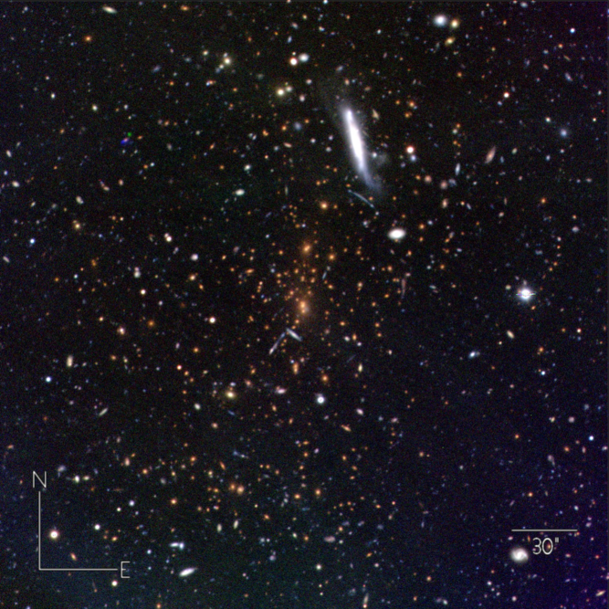
Figure 1.— A composite $gri$ color image of RCS2327  from imaging from the LDSS-3 instrument on Magellan (see § 3.1). The field of view is 2x2 proper Mpc at the redshift of the cluster, centered on the BCG. RCS2327 is obviously demarcated by the abundance of red early-type galaxies in the center of the image. Immediately south of the foreground bright galaxy to the north-northeast is an obvious strongly lensed merging double image (see Section 3.8) which was also readily apparent in the original RCS2 survey data.

Figure 2.— The detection significance versus redshift of RCS2327 compared to the distribution of these properties for clusters from the RCS2 cluster catalog. RCS2327 is indicated as a heavy symbol and is an obvious outlier; it is as significant as any cluster detected at lower redshifts.

3. Followup Observations and Mass Estimates

In this section we describe the multi-wavelength followup observations of RCS2327. Based on these observations, we are able to estimate the mass of RCS2327  from richness, galaxy dynamics, X-ray, Sunyaev Zel’dovich effect, weak lensing and strong lensing. The different mass proxies naturally measure either spherical mass or a projected mass along the line of sight (usually referred to as cylindrical mass or aperture mass). Moreover, each mass proxy is sensitive to mass at a different radial scale: strong lensing measures the projected mass density at the innermost parts of the cluster, typically $\sim$100-500 kpc, and is insensitive to the mass distribution in the outskirts; SZ decrement and X-ray measure the mass at larger radii (typically R₂₅₀₀) and lack the resolution at the center of the cluster; weak lensing reconstructs the projected mass density out to R₂₀₀, with poor resolution at the center as well. Dynamical mass (from the velocity distribution of cluster galaxies) is used to estimate the virial mass. We note that these mass proxies are not always independent, and rely on scaling relations and assumptions. In the following subsections, we describe the data and our analysis to derive the cluster mass from each mass proxy. In § 4 we compare the masses derived from the different mass proxies.

3.1. Deep Multi-color Imaging, Galaxy Distribution and Richness

In addition to the RCS2 survey imaging data, available imaging data on RCS2327 includes images from the LDSS-3 imaging spectrograph on the 6.5m Clay telescope, taken during a run in September 2005. Total integration times were 16, 12, and 10 minutes in the $g$,$r$ and $i$ filters respectively. The point-spread-function width at half maximum in the final stacked images is 0$\farcs$60 ($i$), 0$\farcs$65 ($r$), and 0$\farcs$80 ($g$) with some image elongation due to wind shake present principally in the bluest band. These data cover a circular field of view 8’ in diameter, centered on the BCG. Figure 1 is constructed from these data.

The RCS2 data are best suited to measurements of cluster richness, as they are well calibrated and naturally include excellent background data, and are readily connected to the cosmological context and calibration of the mass-richness relation provided by the RCS1 program (Gladders & Yee, 2005; Gladders et al., 2007). The multi-band LDSS-3 images are deeper, with better seeing than the RCS2 images, and we use these data for computing detailed photometric properties - principally color-magnitude diagrams. For this we focus our analysis below on the $r$ and $i$ observations, since this filter pair has the best image quality, and almost perfectly straddles the 4000Å break at the cluster redshift.

Figure 3.— The color-magnitude diagram for a 1 Mpc radius field of view centered on RCS2327, in the $r$ and $i$ filters. Galaxies have been divided into three radials bins of equal radius; galaxies in the outermost bin are plotted as small pluses, and those in the central bin as heavy squares. Only galaxies with photometric uncertainties in both filters of less than 0.2 magnitudes are shown.

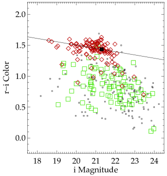
Figure 4.— The color-magnitude diagram for galaxies with spectroscopic redshifts, regardless of position, in the $r$ and $i$ filters. Spectroscopic early-type cluster members are shown as red diamonds; other cluster members are shown as green squares. Non-members are shown as small squares. Only galaxies with uncertainties in both filters of less than 0.2 magnitudes are shown. The best fitting red-sequence model, derived as described in § 3.1, is overplotted with the characteristic magnitude $i^{*}$ indicated by the heavy black square.

Figure 3 shows an $r-i$ color-magnitude diagram of all galaxies at projected radii less than 1 Mpc from the cluster center. The red sequence of early-type cluster members is obvious, emphasizing the extraordinary richness of this cluster in comparison to most other clusters in the literature at a similar redshift (e.g., De Lucia et al., 2007; Gladders & Yee, 2005). Figure 4 shows only galaxies for which a spectroscopic redshift is available, plotted by SED type. As expected, galaxies which are both cluster members and have early-type spectra are almost all red-sequence members. From the spectroscopically confirmed early-type cluster galaxies, with simple iterated 3-$\sigma$ clipping (e.g., as in Gladders et al., 1998), we fit a linear red sequence relation, given by $(r-i)=-0.053\times(i-i^{*})+1.436$. We take the characteristic magnitude for cluster galaxies in RCS2327 as $i^{*}=21.3$, consistent to within 0.05 magnitudes with the models in both Gladders & Yee (2005) and Koester et al. (2007). These models include a correction for passive evolution. The measured scatter of early-type galaxies about the best fit red sequence is less than 0.05, consistent with that seen in other rich clusters at a range of redshifts (Hao et al., 2009; Mei et al., 2009). The best fitting model is indicated in Figure 4. These data demonstrate that RCS2327 appears as expected for a well-formed high-redshift cluster, albeit an extraordinarily rich example.

We derive a total richness for RCS2327 of $B_{gcT}$=3271$\pm$488 Mpc${}_{50}^{1.8}$, and a corresponding red-sequence richness of $B_{gcRS}$=2590$\pm$413 Mpc${}_{50}^{1.8}$ (see Gladders & Yee, 2005, for a detailed explanation of the $B_{gc}$ parameter). Calibrations relevant to the measurement of this richness have been taken from the RCS1 survey, which also uses the $z^{\prime}$-band as the reddest survey filter. A direct comparison of the total richness to the scaling relations in Yee & Ellingson (2003) nominally corresponds to a mass of M${}_{200}=4.6_{-1.1}^{+1.2}\times 10^{15}$ ${h}_{70}^{-1}$M_☉  with a significant uncertainty, given the known scatter in richness as a mass proxy (Gladders et al., 2007; Rozo et al., 2009), and the lack of direct calibration of the richness-mass relation at the redshift of RCS2327. Furthermore, the relevant richness to use in comparison to the scaling relation in Yee & Ellingson (2003) is not obvious; though the richness values in Yee & Ellingson (2003) are for all galaxies, the small blue fraction in that sample and the significant observed evolution in the general cluster blue fraction (Loh et al., 2008) from the redshift of that sample (mean z=0.32) to the redshift of RCS2327 suggests that the (less evolving) red-sequence richness may be a more appropriate measure. With that in mind we note that the mass corresponding to $B_{gcRS}$ is M${}_{200}=3.2_{-0.8}^{+0.9}\times 10^{15}$${h}_{70}^{-1}$M_☉. Given the limitations of this analysis however, we do not use a richness-derived mass extensively in the analysis in § 4, but simply note here that RCS2327 is remarkably rich.

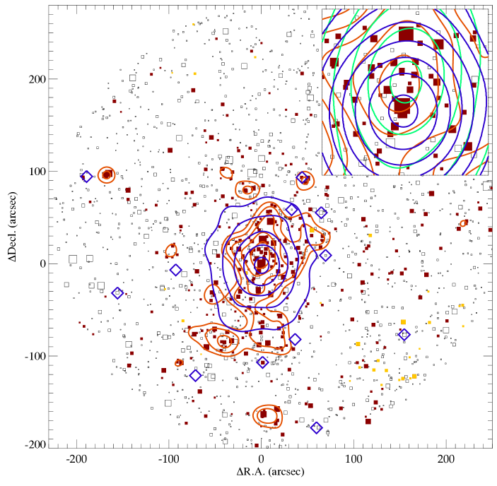
Figure 5.— The distribution of red-sequence galaxy light (red contours) smoothed with a 150 kpc FWHM gaussian, and the full band X-ray light (blue contours) similarly smoothed. Blue diamonds mark X-ray point sources; the correspondance between some of these sources to optical counterparts validates the astrometric matching between these data. Individual galaxies are indicated by squares, with symbol size proportional to brightness; solid red squares have colors consistent with the cluster red-sequence and are the basis for the overplotted contours, and solid yellow squares show spectroscopically confirmed members of the secondary structure noted in Figures 6 and 7 and § 3.2. The inset shows the central 1′$\times$1′region with the same data, with the strong lensing main halo mass distribution also indicated (green contours). The contour levels have been chosen to highlight the core position and outer shape of the light distributions.

3.2. Optical Spectroscopy

Spectroscopic observation of galaxies in the field of RCS2327 has been conducted using the Magellan telescopes. Data were acquired in both normal and nod-and-shuffle modes using LDSS-3, during runs in August and November, 2006, and a total of 3 masks with the GISMO instrument in June 2008. RCS2327 was also observed using the GMOS instrument on the Gemini South telescope in queue mode in semester 2007B, yielding redshifts of potential lensed sources; the Gemini data are discussed in more detail in § 3.8 below.

All Magellan spectra have been reduced using standard techniques, as implemented in the COSMOS pipeline. The bulk of the LDSS-3 observations (apart from a single early mask, which established the cluster redshift at $z\sim 0.70$) were acquired using a 6000Å-7000Å band-limiting filter; this allows for a high density of slits, at the expense of a significant redshift failure rate (specifically, [O II]$\lambda\lambda 3727$  is undetectable outside of $0.61<z<0.87$, and the Ca H and K lines are undetectable outside of $0.53<z<0.76$). The GISMO observations were conducted using a band limiting filter covering 5700Å-9800Å.

A total of 353 robust redshifts were measured from these data. Most are unique, with overlap between observations with different instruments or runs amounting to a few galaxies per mask. From six galaxies in common beween the LDSS-3 and GISMO data the mean difference in redshifts is measured to be 135 km sec^-1, and the uncertainty within observations using a single instrument is measured to be less than 100 km sec^-1. Neither of these uncertainties is significant in the analysis below. Redshifts were measured using a combination of cross correlation and line measurement techniques, and cross correlation measurements of absorption systems were only retained if (at minimum) the H and K lines were individually visible. Apart from possible mis-interpreted single emission line redshifts in the LDSS-3 spectra, the measured redshifts are robust. Each spectrum was also classified as either an emission or absorption type, with post-starburst (showing strong Balmer lines) or AGN features also noted when present.

A histogram of the galaxy velocities around the mean cluster redshift of 0.6986$\pm$0.0005 is shown in Figure 6. The measured velocity dispersion for 195 cluster members is 1563$\pm$95 km sec^-1 with uncertainties measured from a bootstrap analysis. The cluster is well separated from other structures. The velocity dispersion using only the 110 galaxies with early type spectra is 1398$\pm$99 km sec^-1, and similarly using all other cluster members we derive 1757$\pm$139 km sec^-1 – a factor of 1.27$\pm$0.14 larger. These differences are as expected and in line with that observed for relaxed X-ray selected clusters at lower redshifts, where the typical ratio in velocity dispersion of blue to red cluster members is 1.31$\pm$0.13 (Carlberg et al., 1997).

Figure 6.— The velocity distribution of galaxies about the mean cluster redshift for all galaxies (top), absorption line only galaxies (middle), and all emission line galaxies (bottom). Velocity dispersions in the restframe in km sec^-1are as indicated.

The velocity distribution of cluster members versus projected radius, in Figure 7, shows several trends also consistent with that expected for a relaxed cluster. The velocity dispersion is a declining function of cluster-centric radius, an effect most apparent in the early-type galaxies. In non-overlapping radial bins of 0.5 Mpc in radius, and at mean radii of 0.27, 0.71 and 1.27 Mpc, we find velocity dispersions of 1626$\pm$127 km sec^-1, 1268$\pm$147 km sec^-1, and 1034$\pm$201 km sec^-1, respectively. The radial distribution of emission line members relative to absorption line cluster members is also as expected, with proportionately more actively star-forming systems found at large radii. A clear interpretation of this result is difficult given the complexity of the sampling from multiple masks from multiple instruments with differing fields of view, and the weighting of slit assignments toward photometric red-sequence members; the data shown in Figure 7 are at least consistent with expectations. Finally, a KS test of the velocity distribution shows at best marginal evidence for velocity substructure, with the velocity distribution inconsistent with a normal distribution at a modest 1.3 sigma using all galaxies. Using only early type members, there is not even marginal evidence for velocity substructure.

We also note the presence of a secondary structure separated from the main cluster by 5700 km sec^-1. This structure is dominated by emission line galaxies, has a velocity dispersion of 400 km sec^-1, and is located to the edge of the spectroscopic field of view, as can been seen in Figures 5, 6, and 7. It is not significant for any of the analyses below.

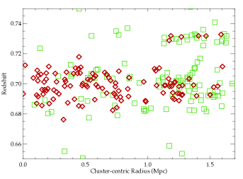
Figure 7.— Redshifts versus cluster-centric radius for absorption-line-only galaxies (red diamonds) and all other galaxies (green squares) for all galaxies within $\Delta z=0.05$ of the RCS2327. The field of view of the GISMO instrument is approximately 0.7 Mpc in these coordinates; the denser sampling this provides in the cluster core, combined with the details of slit placements in the LDSS-3 instrument yields a complex slit weighting with radius which is responsible for the apparent deficit of galaxies at $\sim$1 Mpc.

3.2.1 Dynamical Mass Estimates from Velocity Dispersion

The observed velocity dispersion is converted to mass through the virial scaling relation derived from simulations (Evrard et al., 2008). This relationship is described as

$$M_{200}=\frac{10^{15}}{h(z)}\left(\frac{\sigma_{obs}}{\sigma_{15}}\right)^{\alpha},$$ (1)

where $\sigma_{obs}$ is the observed 1-d velocity dispersion of the cluster, $\sigma_{15}$ is the velocity dispersion normalized for a $10^{15}$M_☉  cluster, and $\alpha$ is the slope of the scaling relation. Evrard et al. (2008) find the best fit parameters for a multitude of cosmologies and velocity dispersions measured from dark matter particles to be $\sigma_{15}=1082.9$ km s^-1 and $\alpha=2.975$. Using this scaling relation with the measured velocity dispersion for all galaxies, the resulting mass is $M_{200}=2.97^{+1.40}_{-0.95}\times 10^{15}$${h}_{70}^{-1}$M_☉. The uncertainties in mass assume a $13\%$ total uncertainty in velocity dispersion. This included both the statistical uncertainty, which is small for the large number of galaxies observed in this sample, and the systematic uncertainty, which includes line-of-sight effects, cluster shape/triaxiality, and foreground/background contamination (Gifford et al. 2013, Saro et al. 2013). Saro et al. (2013) re-fit the scaling relation to a semi-analytic galaxy catalog for the Millennium Simulation and find the parameters to be $\sigma_{15}=938.0$ km s^-1 and $\alpha=2.91$. The resulting mass using these parameters is $M_{200}=3.08^{+1.42}_{-0.97}\times 10^{15}$${h}_{70}^{-1}$M_☉.

3.2.2 Dynamical Mass Estimates from the Caustic Method

The distribution of radial velocities of cluster galaxies as a function of cluster-centric radius can be used to estimate its mass using the caustic technique (Diaferio & Geller 1997, Gifford et al. 2013, Gifford & Miller 2013). This method relies on the expectation that cluster galaxies that have not escaped the potential well of the cluster halo occupy a well-defined region in a radius-velocity phase space confined by the escape velocity from that potential, $v_{esc}(r)$. We follow the techniques outlined in  Gifford et al. (2013), and refer to that publication for a full description of the methods applied here.

Figure 8 shows the radius-velocity space of $\sim 250$ galaxies. We fit an iso-density contour to the data to find $v_{esc}$ as indicated by the velocity edge in phase-space density. The enclosed mass can be derived as

$$GM_{200}=\int^{r_{200}}_{0}\mathcal{F}_{\beta}(r)\mathcal{A}^{2}(r)dr,$$ (2)

where $\mathcal{A}^{2}(r)$ is the square of the line-of-sight escape velocity, and $\mathcal{F}_{\beta}(r)$ is a function of the potential, density, and velocity anisotropy, corrected for projection effects. We apply the common convention of assuming that $\mathcal{F}_{\beta}$ is constant. Physically, this parameter depends on the unknown concentration and velocity anisotropy profile of the cluster. Disagreement on the constant value of $\mathcal{F}_{\beta}$ that results in unbiased mass estimates on average persists in the literature with values ranging from 0.5 to 0.7. Gifford et al. (2013) find that $\mathcal{F}_{\beta}=0.65$ results in mass estimates with less than 4% mass bias for several semi-analytic catalogs available for the Millennium Simulation, and we adopt this value for this study.

We derive a dynamical mass of $M_{200}=2.94^{+1.03}_{-0.76}\times 10^{15}$${h}_{70}^{-1}$M_☉. The uncertainty in the derived mass using the caustics technique depends on the number of galaxies used; from caustic mass analysis of the Millenium Simulation semi-analytic galaxy catalogs, Gifford et al. (2013) find that for $N_{gal}\geq 150$ the scatter is $\leq 30\%$ with a bias of $<4\%$.

We note that the velocity dispersion of galaxies identified as possible members by the caustic technique is $1586\pm 58$ km s^-1, in agreement with the estimates in § 3.2.

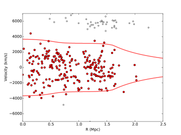
Figure 8.— The projected radius vs line-of-sight velocity phase space for galaxies identified as members by the caustic algorithm (red circles) and non-members (open circles). The estimated escape velocity surfaces (or caustics) are represented by solid red lines which are symmetric with respect to the cluster velocity.

3.3. Chandra Observations, X-ray properties and Mass Estimates

RCS2327 was observed on two separate occasions with the Chandra X-ray Observatory. A first 25 ks observation was carried out on 2007 August 12 (Cycle 8 Proposal 08801039; PI: Gladders) using the ACIS-S array. The early analysis suggested that the cluster was massive, X-ray regular, and possibly hosting a cool core. These hints justified the need of deeper data obtained in 2011 with ACIS-I (Cycle 13 Proposal 13800830; PI: Hicks).

The two deep Cycle 13 ACIS-I pointings (150 ks total) sample a more extended field around the cluster, and result in a higher signal-to-noise ratio than the Cycle 8 observation. Since the background is better understood than that of the ACIS-S configuration, combined with the very small increase in signal-to-noise ratio that would be gained by combining both datasets, we chose to analyse the 2011 data separately and not co-add the two epochs.

The X-ray data reduction follows Martino et al. (2014) and Bartalucci et al. (2014), with minor modifications. We use both the count statistics and the control on systematics offered by a multi-component modeling of the background noise (see Bartalucci et al., 2014, for details). Filtering the hard and soft event light curve reduces the total exposure time by 10% to $\sim 130$ ks. We bin the photon events in sky coordinates with a fixed angular resolution of 1$\farcs$4 and a variable energy resolution that matches the detector response. The effective exposure time and the estimated background noise level are similarly binned. Following the Chandra Calibration database CALDB 4.6.1, when computing the effective exposure we take into account the spatially variable mirror effective area, quantum efficiency of the detector, CCD gaps, bad pixels, and a correction for the motion of the telescope. Our background noise model includes Galactic foreground, cosmic X-ray background, and false detections due to cosmic ray induced particles. For the particle background spectrum, we use the analytical model proposed by Bartalucci et al. (2014). The amplitude of all the other components was determined from the data outside the region of the field of view covered by the target. We derive the temperature map following techniques described in Bourdin & Mazzotta (2008). Figure 9 shows the X-ray flux isophotes overplotted on the false-color temperature map. The cluster has a regular X-ray morphology and does not show significant substructure or X-ray cavities (Hlavacek-Larrondo et al., 2014).

3.3.1 X-ray surface brightness, temperature, and metallicity profiles

We extract the surface brightness profile (Figure 10a) from an effective exposure and background-corrected soft band ([0.5-2.5] keV) image, after excluding point sources. The profile averages the surface brightness in concentric annulli centered on the maximum of a wavelet-filtered image of the cluster. The temperature and metallicity profiles (Figure 10b,c) were calculated in five radial bins out to $\sim 840$ kpc, each containing at least 2000 counts in the [0.7-5] keV band. The measurements of temperature and metallicity assume redshifted and absorbed emission spectra modeled with the Astrophysical Plasma Emission Code (APEC, Smith et al. 2001), adopting the element abundances of Grevesse & Sauval (1998) and neutral hydrogen absorption cross sections of Balucinska-Church & McCammon (1992). The spectra, modified by the effective exposure and background, are also convolved with a function of the redistribution of the photon energies by the detector. The assumed column density value is fixed at $4.73\times 10^{20}$ cm² from measurements obtained near our target by the Leiden/Argentine/Bonn (LAB) Survey of galactic HI (Kalberla et al., 2005). The redshift is fixed to $z=0.6986$.

We find that the metallicity increases from $\sim 0.2$ solar at $R_{\mbox{\scriptsize 2500}}$  to $\sim 0.6$ solar at the cluster core. RCS2327  shows a temperature gradient towards the center of the cluster, indicating a significant cool core. The temperature in the estimated $[0.15-1]\times R_{500}$ region (roughly out to 1Mpc, see § 3.3.2) is $T_{X}=13.9_{-1.8}^{+2.4}$ keV. We also estimate the cooling times as a function of cluster-centric radius (following the prescription described in Hlavacek-Larrondo et al. 2013), and find that the cooling time profile decreases mildly towards the center from $\sim 40$ Gyr at 400 kpc, to $\sim 4$ Gyr at the core. From the gas density (§ 3.3.2) and temperature profile, we find that the central entropy is $46\pm 28$ keV cm^-2.

3.3.2 X-ray Mass Estimate.

To measure the X-ray mass we follow the forward procedure described in Meneghetti et al. (2010) and Rasia et al. (2012). In short, analytic models are fitted to the projected surface density and temperature profiles and subsequently analytically de-projected. The 3D information are then folded into the hydrostatic mass equation (Vikhlinin et al., 2006). The surface brightness is parametrized via a modified $\beta-$model with a power-law trend in the center and a steepening behavior in the outskirts, plus a second $\beta-$model to describe the core:

$$n_{p}n_{e}(r)=n_{0}^{2}\frac{(r/r_{c})^{-\alpha}}{(1+r^{2}/r_{c}^{2})^{3\beta-\alpha/2}}+\frac{n_{02}^{2}}{(1+r^{2}/r_{c2}^{2})^{3\beta_{2}}},$$ (3)

where $n_{e}$ and $n_{p}$ are the electron and proton densities, respectively. We allow all parameters to vary.

We model the temperature profile with a simple power-law:

$$T_{\rm 3D}(r)=T_{0}(r/r_{t})^{-a}.$$ (4)

This profile is then projected along the line of sight using the formula of the spectroscopic-like temperature:

$$T_{\rm los}=\frac{\int WT_{\rm 3D}dV}{\int WdV},$$ (5)

where $W=(n_{p}n_{e})/(T_{\rm 3D}^{0.75})$. All the best fit parameters are determined using a $\chi^{2}$ minimization technique applied to the models and the data. Finally, the 3D density and temperature profiles are used to estimate the total gravitational mass through the equation of hydrostatic equilibrium (HSE; Sarazin 1988):

$$M(r)=-3.68\times 10^{13}T(r)r^{2}\left(\frac{d\log\rho_{g}}{dr}+\frac{d\log T}{dr}\right){\rm h}_{70}^{-1}M_{\odot},$$ (6)

where the numerical factor includes the gravity constant, proton mass, and the mean molecular weight, $\mu=0.5954$.

To estimate the uncertainties, we produce 500 realizations of the surface brightness and temperature profiles assuming a Poisson distribution for the total counts in each annulus and a Gaussian distribution for the projected temperature. The fitting procedure described above is repeated each time. The derived mass profiles are related to the original HSE mass profile via the resulting value of the least-mean-square formula ($=\Sigma[M_{\rm realization}-M_{\rm original}]^{2}$, where the sum extends to all radial bins). We consider the 68% of the profiles (340 in number) with the smallest associated value and, finally, for each radial bin, we consider the maximum and minimum values of the selected profiles. The resulting mass profile and its uncertainties are plotted in Figure 10d. The HSE radius and mass at overdensity $\Delta=$2500 are $R_{2500}=471^{+54}_{-33}$${h}_{70}^{-1}$  kpc, and $M_{2500}=3.2^{+0.6}_{-0.3}\times 10^{14}$${h}_{70}^{-1}$M_☉, respectively, and the gas mass within this radius is $M_{\rm gas,2500}=4.4^{+0.8}_{-0.5}\times 10^{13}$${h}_{70}^{-1}$M_☉.

On average, HSE masses are expected to be biased low by 10-15% as evident from simulations (Rasia et al., 2006; Nagai et al., 2007; Battaglia et al., 2013) and observations (Mahdavi et al., 2008, 2013). This offset is smaller than our statistical uncertainty.

The value of $R_{2500}$ is within the region probed by the observation, and thus its measurement is conservative and robust. However, the lower overdensities $\Delta=500$ and $\Delta=200$ are not within the observed region, and we therefore need to extrapolate. For that purpose, we follow two different approaches.

1: NFW-mass extrapolation

We fit the 500 realizations with the Navarro-Frenk-White (NFW, Navarro et al. 1995, 1996, 1997) formula:

$$M_{\rm NFW}=4\pi M_{0}r_{s}^{3}\left[\log(1+r/r_{s})-\frac{r/r_{s}}{1+(r/r_{s})}\right],$$ (7)

where $r_{s}$ is the scale radius and $M_{0}$ the normalization of the mass profile. The fitting is carried out only within the observed radial region. The results lead to $R_{500}=1.15^{+0.59}_{-0.25}$${h}_{70}^{-1}$  Mpc and $R_{200}=1.78^{+1.24}_{-0.43}$${h}_{70}^{-1}$  Mpc. The errors represent the minimum and maximum values of the 68% of the analytic expressions that are the closest to the NFW fit of the original mass profile. The resulting extrapolated masses are $M_{500}=1.1^{+0.9}_{-0.6}\times 10^{15}$${h}_{70}^{-1}$M_☉ and $M_{200}=1.8^{+1.8}_{-0.7}\times 10^{15}$${h}_{70}^{-1}$M_☉.

2: $M-Y_{X}$ relation.

To derive $R_{500}$ we also apply the iterative method based on the $M-Y_{X}(=M_{\rm gas}\times T_{X})$ relation proposed by Kravtsov et al. (2006). We start with an initial guess for the radius (we consider twice the value of the measured $R_{2500}$). We evaluate the gas mass at that radius from the surface brightness profile and compute the X-ray temperature from the spectra extracted in the spherical shell with maximum and minimum radii equal to the specific radius and 15% its value. The obtained $Y_{X}$ is compared with the $Y_{X}-M$ relation calibrated from hydrostatic mass estimates in a nearby sample of clusters observed with Chandra (Vikhlinin et al., 2009). This returns an estimate of $M_{500}$ and, thus, a new value for $R_{500}$. The process is repeated until convergence in the radius estimate is reached. The resulting radius is $R_{500}=1.27^{+0.10}_{-0.08}$${h}_{70}^{-1}$ Mpc, corresponding to $M_{500}=1.27^{+0.31}_{-0.22}\times 10^{15}$${h}_{70}^{-1}$M_☉.

While the two extrapolation methods agree within errors, we note that the NFW-mass extrapolation results in much larger uncertainty. This is due to the fact that the HSE mass profile is constrained at a small radius (just above $R_{\mbox{\scriptsize 2500}}$) and thus the external slope of the cluster is poorly constrained from X-ray observations.

Figure 9.— A 4’$\times$4’ temperature map of RCS2327, derived from the deep Chandra Cycle 13 data. The image is centered on RA=23:27:27.53, Dec=$-02$:04:35.6. The temperature is indicated by the color scale, in keV. The contours are X-ray flux isophotes. Point sources have been masked. The temperature and flux maps clearly indicate that RCS2327  has a cool core, and a regular morphology, with no significant substructure.

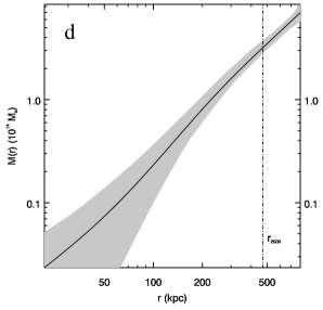
Figure 10.— Radial profiles derived from the analysis of Chandra Cycle 13 150 ks X-ray observation, extended out to 800 kpc. (a) Top-left: Radial profile of the X-ray surface brightness in the soft band [0.5-2.5] keV (data points). The dotted line represents the best fit model. (b) Top-right: Projected temperature profile, clearly showing a temperature decrease towards the center of the cluster, indicating a cool core. The dotted line represents the best fit model. (c) Bottom-left: Metallicity profile (d) Bottom-right: Hydrostatic mass profile (solid line) and its 1-$\sigma$ uncertainty (shaded area). The vertical line indicates $R_{2500}$.

3.4. Sunyaev Zel’dovich Array Observations and SZ Mass Estimates

The Sunyaev Zel’dovich Array (SZA) observed RCS2327 for a total of 48 hours between 2007 September and November. The SZA is an eight-element interferometer with 30 and 90 GHz receivers. The SZA was configured in a standard configuration with 6 telescopes arranged in a compact, short-baseline configuration with two outlying telescopes $\sim$30 m from the central group. The correlated bandwidth was 8 GHz, centered on 31 GHz, resulting in projected lengths of 350$-$1300$\lambda$ on the short (SZ-sensitive) baselines and 2000$-$8000$\lambda$ on the longer baselines. The data were calibrated and flagged using the MATLAB pipeline described in Muchovej et al. (2007); 41% of the data were removed, largely due to shadowing in the compact array, which is increased in equatorial and lower declination objects. The rms noise level in the short-baseline data is 0.21 mJy beam^-1, corresponding to a 15 $\mu$K rms brightness temperature in the 1.9′$\times$ 2.8′ synthesized beam. A bright radio source is detected nearly 9′ to the west of the cluster, but it does not affect the SZ detection. There is one faint radio source coincident with the cluster which we jointly model when presenting data. This source is present in the NRAO VLA Sky Survey (NVSS, Condon 1998). The deconvolved image of the cluster, after subtraction of the radio sources, is shown in Figure 11. The peak significance in this image is 22$\sigma$.

The SZA interferometer acts as a spatial filter sensitive to the Fourier transform of sky emission on angular scales determined by the baseline lengths. To recover the integrated Compton-$y$ parameter, $Y$, we fit our Fourier plane data to the transform of the generalized NFW pressure profile presented in Nagai et al. (2007), which was motivated by simulations and X-ray observations (Mroczkowski et al., 2009). In this five-parameter model we fix the three shape parameters ($\alpha$, $\beta$, $\gamma$) to the best fit values derived from X-ray observations of clusters (1.0620, 5.4807, 1.156; Arnaud et al., 2010). We fit the profile normalization and scale radius. The cluster centroid and the flux of one emissive source are allowed to vary as well. The models are fit to the data directly in the $uv$-plane, which correctly accounts for the noise in the data.

To determine the significance of the cluster detection, we compare the $\chi^{2}$ of the best fit model including the cluster and emissive source with the $\chi^{2}$ of the best fit model including only the emissive source. Expressed in terms of Gaussian standard deviations, the significance of the SZ detection is 30.2$\sigma$.

3.5. Estimates of the Y parameter

We compute two estimates of the $Y$ parameter, $Y_{sph}$ and $Y_{cyl}$. $Y_{sph}$ is a spherical integral of the pressure profile. It is relatively insensitive to unconstrained modes in the interferometer-filtered data and proportional to the total integrated pressure of the cluster, making it a robust observable (see Marrone et al 2011).

To compute $Y_{sph}$, we volume-integrate the radial profile to an overdensity radius, $r_{\Delta}$,

$$Y_{\Delta,sph}=\frac{\sigma_{T}}{m_{e}c^{2}}\int_{0}^{r_{\Delta}}P(r/r_{s})dV,$$ (8)

as in Marrone et al. (2012). We determine the overdensity radius of integration by enforcing consistency with the $Y_{500,sph}-M_{500}$ scaling relation derived by Andersson et al. (2011). To enforce consistency, we iteratively chose the integration radius (and, by extension, the mass) until the mass and $Y_{\Delta}$ lie on the mean relation. This analysis yields $Y_{500,sph}=13.4\pm 1.0\times 10^{-5}~{}\rm{Mpc^{2}}$ with $R_{500}=1.13\pm 0.02~{}\rm{Mpc}$ (this radius is 3-15% smaller than the $R_{500}$ that we derive from extrapolating the X-ray data in Section 3.3).

$Y_{cyl}$ is a cylindrical integral of the pressure profile along the line of sight,

$$Y_{\Delta,cyl}=\frac{\sigma_{T}}{m_{e}c^{2}}\int_{0}^{r_{\Delta}}d\Omega\int_{-\infty}^{\infty}P_{e}dl$$ (9)

(see also Mroczkowski et al., 2009). $Y_{cyl}$ corresponds to the aperture integrated SZ flux, and is sensitive to the line of sight contribution of pressure beyond the radius of interest. For our gNFW fits, the ratio of $Y_{cyl}$/$Y_{sph}$ in the $211\farcs 8$ aperture is $1.0564$. We compute $Y_{500,cyl}$ to directly compare our results with the SZ observations of RCS2327  reported by Hasselfield et al. (2013) with data from the Atacama Cosmology Telescope (ACT). From their “Universal Pressure Profile” (UPP) analysis, which implicitly imposes the $Y-M$ scaling relation of Arnaud (2010), they obtain $Y_{500,cyl}=19.1\pm 0.2\times 10^{-5}~{}\rm{Mpc^{2}}$ within an aperture of $R_{500}=2.8\pm 0.1$ arcmin ($1.22\pm 0.04$ Mpc at the cluster redshift). Using the same aperture, we measure $Y_{500,cyl}=16.8^{+1.6}_{-1.4}\times 10^{-5}~{}\rm{Mpc^{2}}$, within $1.5\sigma$ of the Hasselfield et al. (2013) measurement.

3.6. SZ Mass Estimates

We estimate the cluster mass from the value of $Y_{sph}$ quoted above, which corresponds to $M_{500}=8.5\pm 1.1\times 10^{14}$${h}_{70}^{-1}$M_☉  using the Andersson et al. (2011) scaling relation. The uncertainty assumes 21% scatter in $Y$ at fixed mass in the Andersson et al. (2011) scaling relation (Buddendiek et al., 2014).

We also estimate the cluster mass by applying the method outlined in Mroczkowski (2011, 2012) to the SZA data. This method assumes the gas is virialized and in thermal hydrostatic equilibrium within the cluster gravitational potential. Further, we assume the total matter density $\rho_{\rm tot}$ follows an NFW dark matter profile (Navarro et al., 1995), with the gas density $\rho_{\rm gas}$ is a constant fraction of the total density ($\rho_{\rm gas}=f_{\rm gas}\rho_{\rm tot}$), and the pressure and density profiles are spherically symmetric. This method has been applied successfully and compared with other mass estimates in several works (e.g., Reese et al., 2012; Umetsu et al., 2012; Medezinski et al., 2013). A fit to a gNFW profile described above yields $R_{2500}=0.54\pm 0.01~{}\rm{Mpc}$, $M_{2500}=4.6\pm 0.5\times 10^{14}$${h}_{70}^{-1}$M_☉, assuming an average gas fraction within $R_{2500}$ of $f_{gas}=0.137$ from the x-ray analysis in § 3.3. This method yields $R_{500}=1.15\pm 0.04~{}\rm{Mpc}$, $M_{500}=8.9\pm 0.9\times 10^{14}$${h}_{70}^{-1}$M_☉, assuming an average gas fraction in this radius of $f_{gas}=0.12$ from Menanteau et al. (2012). We estimate a $\sim 10\%$ scatter due to the assumption on average gas fraction value and other model assumptions.

Our mass estimates are consistent with Hasselfield et al. (2013), who measure $M_{500}=9.4\pm 1.5\times 10^{14}$${h}_{70}^{-1}$M_☉  from the UPP Y parameter quoted above. In addition to the UPP mass, Hasselfield et al. (2013) report a range of higher $M_{500}$ estimates based on different scaling relations, $M_{500}=12.5-14.3\times 10^{14}$${h}_{70}^{-1}$M_☉, somewhat higher than our measurement. However, the inconsistency between the higher-mass Hasselfield et al. (2013) values and our measurement is not significantly worse than the inconsistency with their own UPP mass.

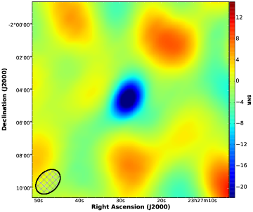
Figure 11.— SZ observation of RCS2327. The CLEANed image is $8\arcmin\times 8\arcmin$ in size. The image is in units of SNR and made from the SZA $uv$-data with a Gaussian $uv$-taper of 0.1 at 4$k\lambda$. The FWHM of the synthesized beam for the image is shown in the bottom left corner. In this image, SNR of 1 corresponds to 0.21$~{}\rm{mJy/bm}$.

3.7. Wide Field Imaging and Weak-Lensing Mass Estimates

We obtained deep wide-field imaging data for RCS2327 in the $i^{\prime}$ filter using Megacam on CFHT with the aim of determining the mass using weak gravitational lensing. The observing strategy and weak lensing analysis follows that of the Canadian Cluster Comparison Project (CCCP; Hoekstra et al., 2012), with the only difference that we use the $i^{\prime}$ for the weak lensing analysis. The $i^{\prime}$ data consist of 8 exposures of 650 s each, which are combined into two sets (each with a total integration time of 2600 s). The pointings in each set are taken with small offsets, such that we can analyse the data on a chip-by-chip basis.

The various steps in the analysis, from object detection to unbiased shape measurements and cluster mass, are described in detail in Hoekstra (2007), with updated procedures in Hoekstra et al. (2015) and we refer the reader to those papers for more details. We measure galaxy shapes as described in Hoekstra et al. (2015), which includes a correction for multiplicative bias based on simulated images. The resulting shapes are estimated to be accurate to $1-2\%$, much smaller than our statistical uncertainties. The shape measurements for each set of exposures are then combined into a master catalog which is used to derive the weak lensing mass. To reduce contamination by cluster members, we also obtained four 720 s exposures in $r^{\prime}$, which are combined into a single image. Galaxies that are located on the cluster red-sequence are removed from the object catalog, which reduces the level of contamination by a factor of two. However, many faint cluster members are blue, and we correct the lensing signal for this residual contamination, as described in Hoekstra (2007).

To quantify the lensing signal, we compute the mean tangential shear as a function of distance from the cluster center using galaxies with $22<i^{\prime}<24.5$. Figure 12 shows the resulting signal, which indicates that the cluster is clearly detected. The bottom panel shows a measure of the lensing ‘B’-mode, which is consistent with zero, indicating that the various corrections for systematic distortions have been properly applied.

Figure 12.— Mean tangential shear as a function of radius from the BCG is shown in the top panel, along with the best fitting isothermal sphere model for reference. The model was fit only to the data at $r>75^{\prime\prime}$ (solid line). The dashed line is the extrapolation of the model to smaller projected radii. The bottom panels shows the ’B’-mode lensing signal, which should be consistent with zero if systematic distortions have been correctly removed.

As discussed in Hoekstra (2007), the weak lensing mass can be derived in a number of ways. However, to relate the lensing signal to a physical mass requires knowledge of the redshift distribution of the galaxies used in the lensing analysis. We use the results from Hoekstra et al. (2015) and find that the mean ratio of angular distances between lens-source and observer-source is $D_{ls}/D_{s}=0.194$.

For reference, we show the best fit singular isothermal sphere model in Figure 12, for which we obtain an Einstein radius ${\rm R}_{\rm E}=10\farcs 1\pm 1\farcs 9$, which yields a velocity dispersion of $\sigma=1345^{+122}_{-134}$ km s^-1 for the adopted source redshift distribution. This value is in excellent agreement with the dynamics inferred from the galaxy redshifts. We also fit an NFW model to the data, adopting the mass-concentration relation suggested by Duffy et al. (2008), which yields a mass M${}_{\rm 200}=2.0^{+0.9}_{-0.8}\times 10^{15}$${h}_{70}^{-1}$M_☉. We compare the weak lensing mass to other mass estimates and in other radii in § 4.2.

3.8. Strong Lensing Mass Estimates

RCS2327 was observed by HST+ACS (Cycle 15 program GO-10846; PI Gladders) as part of a larger effort using both ACS and NICMOS to acquire deep multi-band imaging of this cluster. Unfortunately, the failure of ACS in early 2007 truncated this program, and the only complete image which was acquired is a 3-orbit F435W image of the cluster core taken using the ACS Wide Field Channel. Additional available observations of the cluster core relevant for the strong lensing analysis include a deep ($\sim$2 hours) K-band image of RCS2327 acquired using the PANIC instrument on the Baade Magellan I telescope in 2006, as well as an incomplete 4-pointing mosaic of RCS2327 in the F160W filter taken with HST+NICMOS; we have reconstructed this last image from the useable portions of a nominally failed HST  observation which nevertheless yielded some useful frames in a single orbit before guiding issues truncated the remainder of the observations. A color composite image of the cluster core, made from the F435W image, the deep LDSS-3 $i$-band image (see § 3.1 above), and the PANIC K_s-band image, is shown in Figure 13.

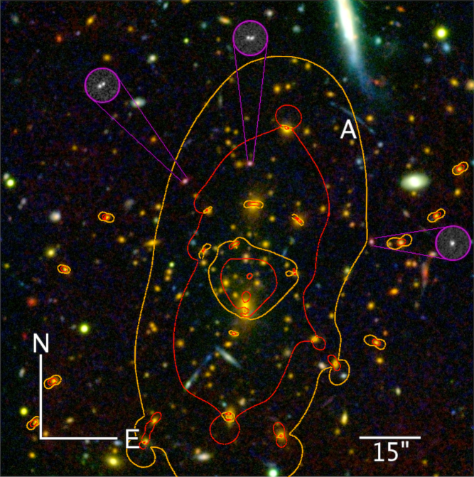
Figure 13.— A 2’$\times$2’ color composite image of the core of RCS2327 composed of images from HST  in the F435W filter (blue channel), and from Magellan in the $i-$band (green channel) and $K_{s}$-band (red channel). The point spread functions have been matched to the worst image; the effective resolution is $\sim 0\farcs 6$. The merging pair image of source A at $z$=2.9834 is indicated. The greyscale cutouts are 2″   in diameter and show the full-resolution images of source B, at $z$=1.4155, in the F435W filter. The critical curves from the best fit lens model are overplotted, in red for a source at $z$=1.415, and in orange for a source at $z$=2.9834.

Using these various imaging data, we identify two sets of multiply-imaged galaxies that are lensed by RCS2327 for which we have acquired spectroscopic redshifts as part of the overall spectroscopic program described in § 3.2. Both sources are indicated in Figure 13. A merging pair of images of source A is located at 23:27:29.43, $-02$:03:47.8, to the NE of the cluster center. Its redshift, $z=2.9834\pm 0.0010$, is determined from a strong Ly$\alpha$ emission line present in the early LDSS-3 spectroscopy described above. This lensed source was apparent in the RCS2 discovery imaging data, with a remarkably large separation from the cluster center, R=56$\farcs$8, as measured from the BCG. The arc does not appear to be caused by local substructure in the cluster, as there are no nearby significant cluster galaxies.

Source B was observed spectroscopically in queue mode in semester 2007B using the Gemini South telescope with the GMOS instrument. We observed RCS2327 for $8\times 1800$s in multi-object spectroscopy mode. The observations were taken with the B600_G2353 grating, no filter, and the detector binned 1$\times$2 (spatial$\times$spectral axes), resulting in wavelength coverage of $\sim 2700$Å per slit, and a spectral resolution of $\sim 240$ km sec^-1. The grating tilt was optimized to record a wavelength range of $\sim 3800-6500$Å  for images of source B.

The redshift of source B is $z=1.4155\pm 0.0008$, based on [O II]$\lambda\lambda 3727$  emission present in a GISMO observation (see § 3.2) confirmed by several FeII lines in absorption in the Gemini spectra. Source B is lensed into three images, and is not morphologically obvious in the discovery data from RCS2327, as it is not lensed into a classic tangential arc. It is apparent in the combined HST  and IR imaging since it has a unique color and internal morphology. These properties also allow us to robustly eliminate the presence of a fourth counter image; source B is lensed as a naked cusp configuration (e.g., Oguri & Keeton, 2004). A close inspection of the F435W image reveals that two of the images (B1 and B2) have two emission knots at their center; overall source B appears to be a compact galaxy with a primarily redder stellar population, but with two well confined regions of active star formation in the galaxy’s core. The detailed position of these bright knots indicates a larger magnification in the tangential direction than in the radial direction for this source. The two knots in the third image are not resolved, but the image is elongated in the tangential direction. Source B also has a significant Einstein radius, with separations for the three images from the cluster BCG of 36$\farcs$8, 36$\farcs$6, and 35$\farcs$8. Further lensed features are also apparent, but we do not yet have redshift information for them and they are not used in the initial lensing model discussed below.

A strong lensing model for RCS2327 was constructed using the publicly available software LENSTOOL (Jullo et al., 2007). The mass model is composed of multiple mass clumps. The cluster halo is represented by a generalized NFW distribution (Navarro et al., 1997), parametrized with position, $x$, $y$; ellipticity $e$; position angle $\theta$; central slope $\alpha$; and concentration $c$. The 50 brightest red-sequence-selected cluster-member galaxies are represented by Pseudo-Isothermal Ellipsoidal Mass Distributions (PIEMD; see Jullo et al., 2007, for details) parametrized with positional parameters ($x$, $y$, $e$, $\theta$) that follow their observed measurements, $r_{\rm{core}}$ fixed at 0.15 pc, and $r_{\rm{cut}}$ and $\sigma_{0}$ scaled with their luminosity (see Limousin et al. 2005 for a description of the scaling relations). The parameters of an L* galaxies were fixed at $r_{cut}=40$ kpc and $\sigma_{0}=160$ km s^-1. The model consists of 13 free parameters. All the parameters of the cluster halo are allowed to vary (R.A., Decl. of the mass clump, ellipticity, position angle, scale radius, concentration and central radial mass profile).

The constraints are the positions of the lensed features and their redshifts. Each component of Arc A was represented by three positions, and the two cores of source B were used in each of its images. The best fit model is determined through Monte Carlo Markov Chain (MCMC) analysis through minimization in the source plane, with a resulting image-plane RMS of 0$\farcs$17. The best fit parameters and their 68% percentile uncertainties are presented in Table 1. Some of the model parameters are not well-constrained by the lensing evidence. In particular, a large range of values is allowed for $r_{s}$ and $\alpha$, and the model can converge on any value of the concentration parameter $c$. The latter is not surprising, since in order to determine the concentration parameter one needs to constrain the slope of the mass profile on small and large radii, beyond the range of the strong lensing constraints. Thus the concentration uncertainty given in Table 1 represents the range of priors assumed in the lens modeling process. We find strong correlations between, $\alpha$, $r_{s}$, and $c$, which we fit to find $r_{s}=575.4-906.8\alpha+583.3\alpha^{2}$  and $c=16.1-8.8\alpha$.

Table 1Best fit Strong Lensing Model Parameters

Halo	Model	RA	Dec	$e$	$\theta$	$r_{\rm s}$	$\alpha$	$c$
		($\arcsec$)	($\arcsec$)		(deg)	(kpc)
Halo 1	gNFW	$1.17^{+0.47}_{-0.24}$	$7.42^{+1.42}_{-0.63}$	$0.26^{+0.04}_{-0.06}$	$102.0^{+0.4}_{-1.0}$	$486^{+62}_{-266}$	$1.44^{+0.09}_{-0.62}$	$3.40^{+5.09}_{-0.40}$

Note. — Coordinates are measured in arcseconds East and North of the center of the BCG, at [RA, Dec]=[351.865026, $-2$.076924]. The ellipticity is expressed as $e=(a^{2}-b^{2})/(a^{2}+b^{2})$. $\theta$ is measured North of West. Error bars correspond to 1-$\sigma$ confidence level as inferred from the MCMC optimization.

The Einstein radius of a lens is often used as a measure of its lensing cross section, or strength. We measure the effective Einstein radius as $R_{E}=\sqrt{A/\pi}$, where $A$ is the area enclosed by the tangential critical curve, $R_{E}(z=1.4155)=25\farcs 9$ for source B, and $R_{E}(z=2.9834)=40\farcs 2$ for the giant arc A. These radii are smaller than the separations between the arcs and the BCG, due to the ellipticity of the lensing potential. The mass that results from the lensing model can be quoted at a range of radii, though it is clear that the mass is most robustly measured at the critical radii probed by the lensed images used to construct the model (e.g. Meneghetti et al., 2010). We integrate the strong lens model within circular apertures at radii corresponding to the mean positions of sources A and B with respect to the position of the main cluster NFW halo, and find enclosed projected mass $M_{cyl}(<R_{A})=$$5.8^{+0.4}_{-0.2}\times 10^{14}$M_☉, $M_{cyl}(<R_{B})=$$3.4^{+0.3}_{-0.1}\times 10^{14}$M_☉. Statistical uncertainties are computed by sampling models described by the MCMC outputs, considering only models with values of $\chi^{2}$ within two of the best fit, representing 1-$\sigma$ uncertainty in the parameter space. The resulting masses are a measure of the projected (i.e., cylindrical) masses within the quoted radii. These statistical uncertainties may fail to reflect some systematics due to the small number of lensing constraints in this system. In particular, since the lens is only constrained by arcs on one side of the cluster, we see correlations in the parameter space between the mass, ellipticity, and position of the lens. The superior data expected from HST  Cycle 20 program GO-13177, will enable a better constrained lens model (Hoag et al., 2015). We adopt a 15% systematic uncertainty from Zitrin et al. (2015) for clusters with similar strong lensing signal.

A notable further result from the strong lens model is that the cluster halo is offset from the BCG by $1.17^{+0.47}_{-0.24}$  and $7.42^{+1.42}_{-0.63}$  arcseconds in right ascension and declination, respectively. This corresponds to an offset of 54 kpc at the cluster redshift. Figure 5 shows the positional relationship between the cluster galaxies – as demarcated by red-sequence members – and both the X-ray data and the strong lensing model. The peak of the X-ray emission is coincident with the position of the BCG as is typically seen in lower redshift relaxed clusters (Sanderson et al., 2009; Bildfell et al., 2008). The center of the overall distribution of the red sequence light is coincident with the strong lensing mass peak, both of which are hence offset from the BCG and the X-ray centroid by $\sim$60 kpc. Disagreements between the mass peak as traced by lensing and the X-ray centroid are seen in major clusters mergers (e.g. Bradač et al., 2008; Mahdavi et al., 2007; Clowe et al., 2004) although the magnitude of the disagreement in RCS2327 is not nearly as large and is similar to that observed in intermediate cooling flow clusters in the sample of clusters in Allen (1998). However, the differing positions indicated by various mass tracers is arguably the strongest evidence that RCS2327 is anything but a single relaxed halo; we explore the implications of this further in § 4.

4. Discussion

The various mass proxies detailed in § 3 all indicate that RCS2327 is an exceptionally massive cluster given its redshift. Each of these mass proxies is naturally sensitive to the mass of RCS2327 at a particular radius, and involves in all cases one or more simplifying assumptions that allow the conversion of the observable signal into a mass estimate. For example, the X-ray data most directly constrain the mass at an overdensity radius of $\sim$R₂₅₀₀ and conversion of the X-ray spectrum and radial luminosity profile to a spherical mass estimate requires the assumption of hydrostatic equilibrium. The strong lensing data are sensitive to mass at similar or smaller radii than the X-ray data, but fundamentally measures a cylindrical mass in projection. The galaxy dynamics are sensitive to mass at the virial scale and rely on external scaling relations to provide a mass estimate, which, as detailed in § 3.2, are sensitive to not well known issues of velocity bias and orbital anisotropies.

4.1. Comparison to Other Clusters

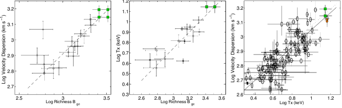
Figure 14.— The comparison of richness, velocity dispersion, and X-ray temperature for RCS2327 (green squares) against relations for these quantities from the literature. The left and middle panels compare to the data and fitted relations in Yee & Ellingson (2003) for velocity dispersion - richness (left) and X-ray temperature - richness (middle) and the right panel compares to the data and fitted relation in Xue & Wu (2000) for velocity dispersion - X-ray temperature. Both the total and early-type-only richnesses are shown, as well as velocity dispersions from both the early-type-only and all galaxies. The X-ray temperature and velocity dispersions (for all galaxies and early-type-only) of ACT-CL J0102–4915  ($z=0.87$) from Menanteau et al. (2013) are plotted in orange circles.

The left and middle panels of Figure 14 compare the velocity dispersion, X-ray temperature and richness of RCS2327 to the global correlations of these properties in an intermediate X-ray selected cluster sample from Yee & Ellingson (2003). The right panel of Figure 14 plots the measured velocity dispersion and X-ray temperature of RCS2327 against the cluster data and fitted relation from Xue & Wu (2000). We plot both the total and red-sequence richnesses, and the velocity dispersion from all galaxies, and only early-type galaxies. Which of each of these properties is best compared to the correlations in Yee & Ellingson (2003) or Xue & Wu (2000) is not obvious (e.g., see § 3.1). Regardless, to within both the measurement uncertainties and these systematic uncertainties, these three measures (which probe large scale dynamics, the gas properties of the cluster core – and hence small scale dynamics, the gas fraction, and the like – and the stellar mass-to-light ratio) are all consistent with a massive cluster with properties drawn from the global correlations seen in large cluster samples.

In Figure 15, reproduced from Bleem et al. (2015), we plot the estimated $M_{500}$ versus the redshift of RCS2327, compared to clusters from large X-ray and SZ cluster surveys. The figure illustrates that RCS2327  is among the most massive clusters at all redshifts, and in particular at $z\geq 0.7$.

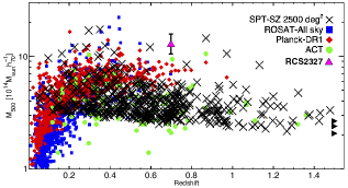
Figure 15.— Reproduced from Bleem et al. (2015). Estimated mass versus redshift for clusters from four large X-ray and SZ surveys: SPT-SZ 2500 deg² (Bleem et al., 2015), ROSAT all sky survey (Piffaretti et al., 2011), Planck-DR1 (Planck Collaboration et al., 2013), and ACT (Marriage et al., 2011). The X-ray mass of RCS2327  ($M_{500}=1.3^{+0.3}_{-0.2}\times 10^{15}$M_☉) is overplotted as a magenta triangle, placing it among the most massive clusters across all redshifts, and comparable to only few other clusters at $z\geq 0.7$. We note that clusters that appear in different catalog may show multiple times on this plot, e.g., ACT-CL J0102–4915  (Marriage et al. (2011), Menanteau et al. (2013)) appears with three mass estimates at $z=0.87$. Other notable high-mass clusters are SPT-CLJ2337-5942 at $z=0.77$, SPT-CLJ0615-5746 at $z=0.972$ and SPT-CLJ2106-5844 at $z=1.132$ (Bleem et al., 2015; Foley et al., 2011; Planck Collaboration et al., 2011).

4.2. Comparison of Mass Proxies

Though each of the mass proxies discussed above measure the mass most naturally at differing radii, it is still instructive to compare the results directly. To do so we consider several additions to the main analyses in § 3. Table 2 summarizes the mass estimates from different mass proxies at different radii, and they are plotted in Figure 16.

4.2.1 Cylindrical Masses from X-ray, Strong and Weak Lensing

As noted above, weak and strong lensing are both sensitive to projected mass density. However, they probe different regimes of the mass distribution: strong lensing is insensitive to the mass at the outskirts of the cluster, where no strong-lensing evidence exists. Weak lensing lacks the resolution at the cluster core. To compare the weak and strong lensing mass estimates, we first compute the projected enclosed mass (also known as the aperture mass) as a function of radius directly from the weak lensing data. We use the $\zeta_{c}$ statistic (Clowe et al., 1998; Hoekstra, 2007) and convert the measurements into projected masses, using the best fit NFW to estimate the large scale mean surface density (see Hoekstra, 2007, for details). The dependence of the resulting projected mass estimate on the assumed density profile is minimal (Hoekstra et al., 2015). At a radius of 500 ${h}_{70}^{-1}$  kpc this yields a projected enclosed mass of $M_{\rm WL,cyl}(<500$${h}_{70}^{-1}$$\rm{kpc})=5.7\pm 1.1\times 10^{14}$${h}_{70}^{-1}$M_☉.

We can similarly extend the mass estimate from the strong lensing model to larger radii. However, since the lens model is only constrained by lensing evidence in the innermost 400 kpc (measured from the BCG) we increase the systematic uncertainty of the strong lensing mass estimate by $\sim$10%. Following the analysis outlined in § 3.1, we find a mass at a 500${h}_{70}^{-1}$kpc radius of $M_{\rm SL,cyl}(<500$${h}_{70}^{-1}$$\rm{kpc})=8.0\pm 1.5\times 10^{14}$${h}_{70}^{-1}$M_☉. These two values are in fair agreement. We refrain from extrapolating the strong lensing mass to larger radii, where the strong lensing model is not constrained.

The X-ray masses can be converted to cylindrical mass, by integrating along the line of sight out to 10 Mpc on both sides of the cluster center. We note that this may introduce some uncertainty as this is model-dependent. The projected enclosed X-ray masses at the radii of the lensed galaxies (see Table 2) are $2.0^{+0.5}_{-0.4}$, $4.0^{+1.2}_{-0.8}$, $6.2^{+2.1}_{-1.4}$$\times 10^{14}$${h}_{70}^{-1}$M_☉  for 271, 352, 500 kpc, respectively. These values are in fair agreement with the projected enclosed masses derived from strong lensing, $3.4^{+0.3}_{-0.1}$, $5.8^{+0.4}_{-0.2}$, $8.0^{+0.6}_{-0.4}$$\times 10^{14}$${h}_{70}^{-1}$M_☉, respectively. The differences are in line with expected uncertainties and biases (see, e.g., Mahdavi et al. 2013) for hydrostatic masses, as overall we find that the lensing masses are somewhat higher than the X-ray and SZ masses. Nevertheless, it may also indicate that structure along the line of sight or elongation of the cluster halo may be significant. For example, the structure that is indicated by a concentration of galaxies at $z\sim 0.73$ (Figure 7) may be contributing to the lensing signal, and should be accounted for in future lensing analysis (D’Aloisio et al., 2014; McCully et al., 2014; Bayliss et al., 2014a).

4.2.2 Spherical Masses

To compare the weak lensing, X-ray, and SZ masses we deproject the aperture masses following Hoekstra (2007), assuming the mass-concentration from Duffy et al. (2008). Although the deprojection is somewhat model dependent, it is less sensitive to deviations from the NFW profile. At the cluster core, we compute the corresponding deprojected weak lensing mass within 500 ${h}_{70}^{-1}$ kpc (approximately $R_{2500}$). We obtain a value of $M_{\rm WL}(<500$${h}_{70}^{-1}$${\rm kpc})=4.1^{+1.2}_{-1.1}\times 10^{14}$${h}_{70}^{-1}$M_☉  within this radius, in agreement with the X-ray estimate of $M_{\rm{X},2500}=3.2^{+0.6}_{-0.3}\times 10^{14}$${h}_{70}^{-1}$M_☉, and SZ mass of $M_{\rm{SZ},2500}=4.6\pm 0.5\times 10^{14}$${h}_{70}^{-1}$M_☉.

At large radii, we use the extrapolated X-ray mass as described in § 3.3. In making this comparison we note that the native values of $R_{200}$ from each of these analyses agree within the uncertainties. The X-ray mass is $M_{\rm{X},200}=1.8^{+1.8}_{-0.7}\times 10^{15}$${h}_{70}^{-1}$M_☉  and the weak lensing mass from the NFW fit is $M_{\rm{WL},200}(<2.1\rm{Mpc})=2.7\pm 0.7\times 10^{15}$${h}_{70}^{-1}$M_☉. Hence at large radii the extrapolated X-ray mass and weak lensing data also agree within the uncertainties.

Table 2 Estimated Masses

Mass proxy	Projected Mass [$10^{14}$${h}_{70}^{-1}$M☉]			Spherical Mass †
	$R=217$kpc	$R=352$kpc	$R=500$kpc	$r_{2500}$	$M_{2500}/10^{14}$	$r_{500}$	$M_{500}/10^{14}$	$r_{200}$	$M_{200}/10^{14}$
				[kpc]	[${h}_{70}^{-1}$M☉]	[Mpc]	[${h}_{70}^{-1}$M☉]	[Mpc]	[${h}_{70}^{-1}$M☉]
Strong Lensing	$3.4^{+0.3}_{-0.1}$$\pm 0.5$	$5.8^{+0.4}_{-0.2}$$\pm 0.9$	[$8.0^{+0.6}_{-0.4}$$\pm 1.4$]	$\cdots$	$\cdots$	$\cdots$	$\cdots$	$\cdots$	$\cdots$
X-ray	$2.0^{+0.5}_{-0.4}$	$4.0^{+1.2}_{-0.8}$	$6.2^{+2.1}_{-1.4}$	$471^{+54}_{-33}$	$3.2^{+0.6}_{-0.3}$	[$1.15^{+0.59}_{-0.25}$]	[$11^{+9}_{-6}$]	[$1.78^{+1.24}_{-0.43}$]	[$18^{+18}_{-7}$]
Weak Lensing	$\cdots$	$\cdots$	$5.7\pm 1.1$	517	$4.3\pm 1.2$	1.34	$15^{+2.9}_{-2.7}$	$\cdots$	$20^{+9}_{-7}$
SZ	$\cdots$	$\cdots$	$\cdots$	$\cdots$	$\cdots$	$1.13\pm 0.02$	$8.5\pm 0.4$	$\cdots$	$\cdots$
SZ (M11‡)	$\cdots$	$\cdots$	$\cdots$	$540\pm 6$	$4.6^{+0.1}_{-0.2}$	$1.15\pm 0.02$	$8.9\pm 0.8$	$\cdots$	$\cdots$
Velocity dispersion	$\cdots$	$\cdots$	$\cdots$	$\cdots$	$\cdots$	$\cdots$	$\cdots$	2.1	$29.7^{+14}_{-9.5}$
Caustics	$\cdots$	$\cdots$	$\cdots$	$\cdots$	$\cdots$	$\cdots$	$\cdots$	2.1	$29^{+10}_{-7}$
Richness	$\cdots$	$\cdots$	$\cdots$	$\cdots$	$\cdots$	$\cdots$	$\cdots$	2.1	$32^{+9}_{-8}$

Note. — Summary of the mass estimates from the different mass proxies considered in this work. Square brackets indicate extrapolated values. Projected X-ray mass was computed by integrating the mass model along the line of sight out to 10 Mpc on both sides of the cluster.

^† The different mass proxies were estimated within different radii, as indicated.

^‡ SZ measurments using the method of Mroczkowski (2011).

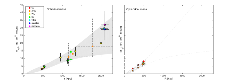
Figure 16.— The mass estimates from the different mass proxies considered in this work (see Table 2) are plotted as a function of radius, color-coded by mass proxy as indicated in the legend. Points with dashed error bars are from extrapolated results (see text). The SZ mass estimates from Hasselfield et al. (2013) are plotted at $R=1.2$ Mpc in green squares. In the left panel we plot spherical masses within radius $r$, and in the right panel are cylindrical (projected) masses enclosed within projected radius $R$. 1-$\sigma$ uncertainties are shown; we note that when $r_{\Delta}$ and $M_{\Delta}$ are determined jointly their uncertainties are correlated. The shaded area in the left panel is the 1-$\sigma$ range of spherical NFW mass profiles that were fit to the spherical masses measured in this work. The measurements that were included in the fit are indicated with thick circles and errorbars. The cylindrical masses in the right panel were not included in the fit, nevertheless, we show the projected mass density of the same fits as striped area in the right panel. As discussed in Section 4.3, this simple fit does not represent a true joint analysis of the data, since various assumptions on the slope of the mass profile are already folded into some of these measurements.

4.3. Mass Profile

Figure 16 presents the enclosed masses measured in this paper as a function of cluster-centric radius, as well as SZ masses from the literature. As demonstrated above, these measurements are consistent with each other within errors, and trace the mass profile from the very core out to $R_{200}$.

We fit a set of spherical NFW profiles (Eq. 7) to the spherical masses measured in this paper. To estimate the range of fits that are consistent with the measurements, we fit the profile 1000 times, each time to a set of measurements that were randomly sampled from their 1-$\sigma$ uncertainties, and weighted by their uncertainties. We did not include in the fit the extrapolated estimates and constraints from the literature. These masses are shown in Figure 16 for reference, extrapolated measurements with in dashed error bars, and the Hasselfield et al. (2013) mass estimates in thin lines. A large range of scale radii is consistent with the measured masses, and the resulting range of NFW profiles is shown as the solid shaded area in Figure 16. The striped area in the right panel of Figure 16 traces the cylindrical mass from the same NFW profiles that were fit to the spherical masses. While we could simultaneously fit the profile to the cylindrical and spherical masses, we choose not to, because the cylindrical strong lensing measurements do not assume spherical symmetry and thus should not be expected to be described by a spherical NFW profile. We find that the strong lensing masses are somewhat higher than the predicted cylindrical masses, which could be due to the triaxiality that is not taken into account in this simplified fit. As expected, the projected X-ray masses do agree with the spherical profile, since they were computed by integration of the X-ray best fit spherical profile along the line of sight.

The simplistic NFW fit to all the non-extrapolated cylindrical mass measurements yields $r_{s}=0.9_{-0.7}^{+1.3}{\rm Mpc}$. However, while a fit of a spherical NFW profile to the mass measurements is possible (though a large range of scale radii is consistent with the results), we caution that such a fit is not meaningful at this point. The different measurements were conducted completely independently of each other, and rely on different assumptions as described in the previous sections (e.g., mass-concentration relations, spherical symmetry, hydrostatic equilibrium, various scaling relations). In particular, some of the mass proxies already assume a certain mass profile slope. A self-consistent combined multi-wavelength analysis is called for. Such an analysis would ideally allow triaxial symmetry, and fit the mass distribution simultaneously to constraints derived directly from all the observables: strong lensing constraints, weak lensing shear, galaxy velocity distribution, and X-ray and SZ measurements. This sort of analysis is left for future work, and is not within the scope of this paper.

5. Summary and Conclusions

We present a multi-wavelength analysis of RCS2327, a massive cluster at $z=0.6986$. The mass is estimated independently at several radii, using seven different mass proxies. At the core of the cluster, we measure the projected mass from a strong lensing model; at intermediate radii, $\sim 0.5$ Mpc, the mass is estimated from X-ray, weak lensing, and the SZ effect. At large radii, $\sim 2$ Mpc, we measure the cluster mass from its weak lensing signal, the dynamics of galaxies in the cluster, and from scaling relations with the richness of the cluster. This analysis provides a unique opportunity of comparing methods and testing them against each other at a significant redshift. In the previous section we compared mass estimates at overlapping radii. Each of the mass proxies is prone to statistical and systematical uncertainties. Moreover, since all the measurements were conducted independently from each other, some of the mass proxies rely on assumptions (e.g., assumed mass-concentration relation or the derived value of $r_{\Delta}$) that are not necessarily uniform among these proxies. This unavoidably contributes to the scatter among the derived masses. Nevertheless, the simple internal comparisons in § 4.2, and the comparison to global cluster correlations in § 4.1 suggests that RCS2327 is not a peculiar object (apart from its overall mass) and we thus expect that a self consistent analysis would yield results comparable to those presented here.

In summary, all the evidence point to the conclusion that RCS2327 is one of the most massive high redshift clusters known to date at $z\geq 0.7$.

The set of measurements presented in this paper is expected to be improved upon in the near future, with deep HST  observations that have already been executed. Further observations will provide constraints for a self-consistent modeling of the three-dimensional cluster mass distribution (e.g., Umetsu et al., 2015; Limousin et al., 2013; Sereno et al., 2013), that takes into account the effects of triaxiality and orientation on the mass observables.

References

- Allen (1998) Allen, S. W. 1998, MNRAS, 296, 392
- Andersson et al. (2011) Andersson, K., Benson, B. A., Ade, P. A. R., et al. 2011, ApJ, 738, 48
- Applegate et al. (2014) Applegate, D. E., von der Linden, A., Kelly, P. L., et al. 2014, MNRAS, 439, 48
- Arnaud (1996) Arnaud, K.A. 1996, ADASS, 101, 5
- Arnaud et al. (2010) Arnaud, M., Pratt, G. W., Piffaretti, R., et al. 2010, A&A, 517, AA92
- Bahcall & Fan (1998) Bahcall, N. A., & Fan, X. 1998, ApJ, 504, 1
- Balucinska-Church & McCammon (1992) Balucinska-Church, M., & McCammon, D. 1992, ApJ, 400, 699
- Bartalucci et al. (2014) Bartalucci, I., Mazzotta, P., Bourdin, H., & Vikhlinin, A. 2014, A&A, 566, A25
- Battaglia et al. (2013) Battaglia, N., Bond, J. R., Pfrommer, C., & Sievers, J. L. 2013, ApJ, 777, 123
- Bayliss et al. (2014b) Bayliss, M. B., Ashby, M. L. N., Ruel, J., et al. 2014b, ApJ, 794, 12
- Bayliss et al. (2014a) Bayliss, M. B., Johnson, T., Gladders, M. D., Sharon, K., & Oguri, M. 2014a, ApJ, 783, 41
- Bildfell et al. (2008) Bildfell, C., Hoekstra, H., Babul, A., & Mahdavi, A. 2008, MNRAS, 389, 1637
- Bleem et al. (2015) Bleem, L. E., Stalder, B., de Haan, T., et al. 2015, ApJS, 216, 27
- Bonamente et al. (2008) Bonamente, M., Joy, M., LaRoque, S. J., Carlstrom, J. E., Nagai, D., & Marrone, D. P. 2008, ApJ, 675, 106
- Bourdin & Mazzotta (2008) Bourdin, H., & Mazzotta, P. 2008, A&A, 479, 307
- Bradač et al. (2008) Bradač, M., Allen, S. W., Treu, T., Ebeling, H., Massey, R., Morris, R. G., von der Linden, A., & Applegate, D. 2008, ApJ, 687, 959
- Brodwin et al. (2014) Brodwin, M., Greer, C. H., Leitch, E. M., et al. 2014, arXiv:1410.2355
- Brodwin et al. (2012) Brodwin, M., Gonzalez, A. H., Stanford, S. A., et al. 2012, ApJ, 753, 162
- Brodwin et al. (2011) Brodwin, M., Stern, D., Vikhlinin, A., et al. 2011, ApJ, 732, 33
- Brodwin et al. (2006) Brodwin, M., Brown, M. J. I., Ashby, M. L. N., et al. 2006, ApJ, 651, 791
- Buddendiek et al. (2014) Buddendiek, A., Schrabback, T., Greer, C. H., et al. 2014, arXiv:1412.3304
- Carlberg et al. (1997) Carlberg, R. G., et al. 1997, ApJ, 476, L7
- Clowe et al. (1998) Clowe, D., Luppino, G. A., Kaiser, N., Henry, J. P., & Gioia, I. M. 1998, ApJ, 497, L61
- Clowe et al. (2004) Clowe, D., Gonzalez, A., & Markevitch, M. 2004, ApJ, 604, 596
- Condon et al. (1998) Condon, J. J., Cotton, W. D., Greisen, E. W., et al. 1998, AJ, 115, 1693
- Crocce et al. (2010) Crocce, M., Fosalba, P., Castander, F. J., & Gaztañaga, E. 2010, MNRAS, 403, 1353
- D’Aloisio et al. (2014) D’Aloisio, A., Natarajan, P., & Shapiro, P. R. 2014, MNRAS, 445, 3581
- De Lucia et al. (2007) De Lucia, G., et al. 2007, MNRAS, 374, 809
- Diaferio & Geller (1997) Diaferio, A., & Geller, M. J. 1997, ApJ, 481, 633
- Duffy et al. (2008) Duffy, A. R., Schaye, J., Kay, S. T., & Dalla Vecchia, C. 2008, MNRAS, 390, L64
- Ebeling et al. (2001) Ebeling, H., Edge, A. C., & Henry, J. P. 2001, ApJ, 553, 668
- Eisenhardt et al. (2008) Eisenhardt, P. R. M., Brodwin, M., Gonzalez, A. H., et al. 2008, ApJ, 684, 905
- Eke et al. (1996) Eke, V. R., Cole, S., & Frenk, C. S. 1996, MNRAS, 282, 263
- Elston et al. (2006) Elston, R. J., Gonzalez, A. H., McKenzie, E., et al. 2006, ApJ, 639, 816
- Evrard et al. (2008) Evrard, A. E., et al. 2008, ApJ, 672, 122
- Foley et al. (2011) Foley, R. J., Andersson, K., Bazin, G., et al. 2011, ApJ, 731, 86
- Gettings et al. (2012) Gettings, D. P., Gonzalez, A. H., Stanford, S. A., et al. 2012, ApJ, 759, L23
- Gifford et al. (2013) Gifford, D., Miller, C., & Kern, N. 2013, ApJ, 773, 116
- Gifford & Miller (2013) Gifford, D., & Miller, C. J. 2013, ApJ, 768, L32
- Gilbank et al. (2011) Gilbank, D. G., Gladders, M. D., Yee, H. K. C., & Hsieh, B. C. 2011, AJ, 141, 94
- Gioia & Luppino (1994) Gioia, I. M., & Luppino, G. A. 1994, ApJS, 94, 583
- Gladders et al. (1998) Gladders, M. D., Lopez-Cruz, O., Yee, H. K. C., & Kodama, T. 1998, ApJ, 501, 571
- Gladders & Yee (2005) Gladders, M. D., & Yee, H. K. C. 2005, ApJS, 157, 1
- Gladders et al. (2007) Gladders, M. D., Yee, H. K. C., Majumdar, S., Barrientos, L. F., Hoekstra, H., Hall, P. B., & Infante, L. 2007, ApJ, 655, 128
- Gralla et al. (2011) Gralla, M. B., Sharon, K., Gladders, M. D., et al. 2011, ApJ, 737, 74
- Grevesse & Sauval (1998) Grevesse, N., & Sauval, A. J. 1998, Space Sci. Rev., 85, 161
- Hao et al. (2009) Hao, J., et al. 2009, ApJ, 702, 745
- Hasselfield et al. (2013) Hasselfield, M., Hilton, M., Marriage, T. A., et al. 2013, Journal of Cosmology and Astroparticle Physics, 7, 008
- Hennawi et al. (2007) Hennawi, J. F., Dalal, N., Bode, P., & Ostriker, J. P. 2007, ApJ, 654, 714
- Hlavacek-Larrondo et al. (2013) Hlavacek-Larrondo, J., Allen, S. W., Taylor, G. B., et al. 2013, ApJ, 777, 163
- Hlavacek-Larrondo et al. (2014) Hlavacek-Larrondo, J., McDonald, M., Benson, B. A., et al. 2015, ApJ, 805, 35
- Hoag et al. (2015) Hoag, A., Bradač, M., Huang, K.-H., et al. 2015, arXiv:1503.02670
- Hoekstra (2007) Hoekstra, H. 2007, MNRAS, 379, 317
- Hoekstra et al. (2012) Hoekstra, H., Mahdavi, A., Babul, A., & Bildfell, C. 2012, MNRAS, 427, 1298
- Hoekstra et al. (2015) Hoekstra, H., Herbonnet, R., Muzzin, A., et al. 2015, MNRAS, 449, 685
- Jee & Tyson (2009) Jee, M. J., & Tyson, J. A. 2009, ApJ, 691, 1337
- Jullo et al. (2007) Jullo, E., Kneib, J.-P., Limousin, M., Elíasdóttir, Á., Marshall, P. J., & Verdugo, T. 2007, New Journal of Physics, 9, 447
- Kalberla et al. (2005) Kalberla, P. M. W., Burton, W. B., Hartmann, D., et al. 2005, A&A, 440, 775
- Koester et al. (2007) Koester, B. P., et al. 2007, ApJ, 660, 239
- Komatsu et al. (2009) Komatsu, E., et al. 2009, ApJS, 180, 33
- Kravtsov et al. (2006) Kravtsov, A. V., Vikhlinin, A., & Nagai, D. 2006, ApJ, 650, 128
- Limousin et al. (2005) Limousin, M., Kneib, J.-P., & Natarajan, P. 2005, MNRAS, 356, 309 Page 17
- Limousin et al. (2013) Limousin, M., Morandi, A., Sereno, M., et al. 2013, Space Sci. Rev., 177, 155
- Loh et al. (2008) Loh, Y.-S., Ellingson, E., Yee, H. K. C., Gilbank, D. G., Gladders, M. D., & Barrientos, L. F. 2008, ApJ, 680, 214
- Mahdavi et al. (2013) Mahdavi, A., Hoekstra, H., Babul, A., et al. 2013, ApJ, 767, 116
- Mahdavi et al. (2008) Mahdavi, A., Hoekstra, H., Babul, A., & Henry, J. P. 2008, MNRAS, 384, 1567
- Mahdavi et al. (2007) Mahdavi, A., Hoekstra, H., Babul, A., Balam, D. D., & Capak, P. L. 2007, ApJ, 668, 806
- Marriage et al. (2011) Marriage, T. A., Acquaviva, V., Ade, P. A. R., et al. 2011, ApJ, 737, 61 Marrone et al. 2011 should be 2012
- Marrone et al. (2012) Marrone, D. P., Smith, G. P., Okabe, N., et al. 2012, ApJ, 754, 119
- Marrone et al. (2012) Marrone, D. P., Smith, G. P., Okabe, N., et al. 2012, ApJ, 754, 119
- Martino et al. (2014) Martino, R., Mazzotta, P., Bourdin, H., et al. 2014, MNRAS, 443, 2342
- Maughan et al. (2004) Maughan, B. J., Jones, L. R., Ebeling, H., & Scharf, C. 2004, MNRAS, 351, 1193
- McCully et al. (2014) McCully, C., Keeton,C. R., Wong, K. C., & Zabludoff, A. I. 2014, MNRAS, 443, 3631
- Medezinski et al. (2013) Medezinski, E., Umetsu, K., Nonino, M., et al. 2013, ApJ, 777, 43
- Mei et al. (2009) Mei, S., et al. 2009, ApJ, 690, 4
- Menanteau et al. (2012) Menanteau, F., Hughes, J. P., Sifón, C., et al. 2012, ApJ, 748, 7
- Menanteau et al. (2013) Menanteau, F., Sifón, C., Barrientos, L. F., et al. 2013, ApJ, 765, 67
- Meneghetti et al. (2010) Meneghetti, M., Rasia, E., Merten, J., et al. 2010, A&A, 514, A93
- Mroczkowski et al. (2009) Mroczkowski, T., et al. 2009, ApJ, 694, 1034
- Mroczkowski (2011) Mroczkowski, T. 2011, ApJ, 728, L35
- Mroczkowski (2012) Mroczkowski, T. 2012, ApJ, 746, L29
- Muchovej et al. (2007) Muchovej, S., et al. 2007, ApJ, 663, 708
- Mullis et al. (2005) Mullis, C. R., Rosati, P., Lamer, G., et al. 2005, ApJ, 623, L85
- Muzzin et al. (2009) Muzzin, A., Wilson, G., Yee, H. K. C., et al. 2009, ApJ, 698, 1934
- Nagai et al. (2007) Nagai, D., Kravtsov, A. V., & Vikhlinin, A. 2007, ApJ, 668, 1
- Navarro et al. (1995) Navarro, J. F., Frenk, C. S., & White, S. D. M. 1995, MNRAS, 275, 720
- Navarro et al. (1996) Navarro, J. F., Frenk, C. S., & White, S. D. M. 1996, ApJ, 462, 563
- Navarro et al. (1997) Navarro, J. F., Frenk, C. S., & White, S. D. M. 1997, ApJ, 490, 493
- Oguri & Keeton (2004) Oguri, M., & Keeton, C. R. 2004, ApJ, 610, 663
- Papovich et al. (2010) Papovich, C., Momcheva, I., Willmer, C. N. A., et al. 2010, ApJ, 716, 1503
- Piffaretti et al. (2011) Piffaretti, R., Arnaud, M., Pratt, G. W., Pointecouteau, E., & Melin, J.-B. 2011, A&A, 534, A109
- Planck Collaboration et al. (2013) Planck Collaboration, Ade, P. A. R., Aghanim, N., et al. 2014, A&A, 571, A20
- Planck Collaboration et al. (2011) Planck Collaboration, Ade, P. A. R., Aghanim, N., et al. 2011, A&A, 536, A8
- Pratt et al. (2009) Pratt, G. W., Croston, J. H., Arnaud, M., Böhringer, H. 2009, A&A, 498, 361
- Rasia et al. (2006) Rasia, E., Ettori, S., Moscardini, L., et al. 2006, MNRAS, 369, 2013
- Rasia et al. (2012) Rasia, E., Meneghetti, M., Martino, R., et al. 2012, New Journal of Physics, 14, 055018
- Reese et al. (2012) Reese, E. D., Mroczkowski, T., Menanteau, F., et al. 2012, ApJ, 751, 12
- Reichardt et al. (2013) Reichardt, C. L., Stalder, B., Bleem, L. E., et al. 2013, ApJ, 763, 127
- Romer et al. (2000) Romer, A. K., et al.2000, ApJS, 126, 209
- Rosati et al. (2009) Rosati, P., Tozzi, P., Gobat, R., et al. 2009, A&A, 508, 583
- Rosati et al. (2004) Rosati, P., Tozzi, P., Ettori, S., et al. 2004, AJ, 127, 230
- Rosati et al. (1998) Rosati, P., della Ceca, R., Norman, C., & Giacconi, R. 1998, ApJ, 492, L21
- Rozo et al. (2009) Rozo, E., et al. 2009, ApJ, 699, 768
- Sanderson et al. (2009) Sanderson, A. J. R., Edge, A. C., & Smith, G. P. 2009, MNRAS, 398, 1698
- Santos et al. (2011) Santos, J. S., Tozzi, P., & Rosati, P. 2011, Memorie della Societa Astronomica Italiana Supplementi, 17, 66
- Sarazin (1988) Sarazin, C. L. 1988, Cambridge Astrophysics Series, Cambridge: Cambridge University Press, 1988,
- Saro et al. (2013) Saro, A., Mohr, J. J., Bazin, G., & Dolag, K. 2013, ApJ, 772, 47
- Sartoris et al. (2010) Sartoris, B., Borgani, S., Fedeli, C., et al. 2010, MNRAS, 407, 2339
- Sereno et al. (2013) Sereno, M., Ettori, S., Umetsu, K., & Baldi, A. 2013, MNRAS, 428, 2241
- Smith et al. (2001) Smith, R. K., Brickhouse, N. S., Liedahl, D. A., & Raymond, J. C. 2001, ApJ, 556, L91
- Stanford et al. (2005) Stanford, S. A., Eisenhardt, P. R., Brodwin, M., et al. 2005, ApJ, 634, L129
- Stanford et al. (2006) Stanford, S. A., et al.2006, ApJ, 646, L13
- Stanford et al. (2012) Stanford, S. A., Brodwin, M., Gonzalez, A. H., et al. 2012, ApJ, 753, 164
- Stanford et al. (2014) Stanford, S. A., Gonzalez, A. H., Brodwin, M., et al. 2014, ApJS, 213, 25
- Staniszewski et al. (2009) Staniszewski, Z.,Ade, P. A. R., Aird, K. A., et al. 2009, ApJ, 701, 32
- Staniszewski et al. (2009) Staniszewski, Z., Ade, P. A. R., Aird, K. A., et al. 2009, ApJ, 701, 32
- Umetsu et al. (2012) Umetsu, K., Medezinski, E., Nonino, M., et al. 2012, ApJ, 755, 56
- Umetsu et al. (2015) Umetsu, K., Sereno, M., Medezinski, E., et al. 2015, ApJ, 806, 207
- Vanderlinde et al. (2010) Vanderlinde, K., Crawford, T. M., de Haan, T., et al. 2010, ApJ, 722, 1180
- Vikhlinin et al. (2006) Vikhlinin, A. et al. 2006, ApJ, 640, 691
- Vikhlinin et al. (2006) Vikhlinin, A., Kravtsov, A., Forman, W., et al. 2006, ApJ, 640, 691
- Vikhlinin et al. (2009) Vikhlinin, A., Burenin, R. A., Ebeling, H., et al. 2009, ApJ, 692, 1033
- Williamson et al. (2011) Williamson, R., Benson, B. A., High, F. W., et al. 2011, ApJ, 738, 139
- Wilson et al. (2009) Wilson, G., et al. 2009, ApJ, 698, 1943
- Wittman et al. (2006) Wittman, D., Dell’Antonio, I. P., Hughes, J. P., Margoniner, V. E., Tyson, J. A., Cohen, J. G., & Norman, D. 2006, ApJ, 643, 128
- Xue & Wu (2000) Xue, Y.-J., & Wu, X.-P. 2000, ApJ, 538, 65
- Yee & Ellingson (2003) Yee, H. K. C., & Ellingson, E. 2003, ApJ, 585, 215
- York et al. (2000) York, D. G., et al. 2000, AJ, 120, 1579
- Zeimann et al. (2012) Zeimann, G. R., Stanford, S. A., Brodwin, M., et al. 2012, ApJ, 756, 115
- Zitrin et al. (2015) Zitrin, A., Fabris, A., Merten, J., et al. 2015, ApJ, 801, 44