Dynamical Detection of Topological Phase Transitions in Short-Lived Atomic Systems

Abstract

We demonstrate that dynamical probes provide direct means of detecting the topological phase transition (TPT) between conventional and topological phases, which would otherwise be difficult to access because of loss or heating processes. We propose to avoid such heating by rapidly quenching in and out of the short-lived topological phase across the transition that supports gapless excitations. Following the quench, the distribution of excitations in the final conventional phase carries signatures of the TPT. We apply this strategy to study the TPT into a Majorana-carrying topological phase predicted in one-dimensional spin-orbit-coupled Fermi gases with attractive interactions. The resulting spin-resolved momentum distribution, computed by self-consistently solving the time-dependent Bogoliubov–de Gennes equations, exhibits Kibble-Zurek scaling and Stückelberg oscillations characteristic of the TPT. We discuss parameter regimes where the TPT is experimentally accessible.

Systems of ultracold atoms provide one of the most versatile platforms for realizing many-body quantum phases of matter. In fact, several quantum phases and phase transitions such as the superfluid-Mott transition Jaksch ; Greiner ; Folling ; Spielman ; Campbell ; Bakr have been realized in such systems. Yet, many of the most interesting phases or phase transitions in such systems are yet to be observed. One of the most glaring examples is the elusive antiferromagnetic Néel order Greif ; Hart in the fermionic Hubbard model, which is believed to be a precursor of superconductivity in the model. Another example is the recently proposed family of phases based on the realization of spin-orbit coupling (SOC) by artificial gauge fields lin ; wang ; cheuk ; Zhang1 ; Qu , which includes topological insulators Beri ; Spielman12 ; Lewenstein , topological superfluids (TSFs) Liang ; Liuxj ; Wei ; Zhang ; Sato ; jay11 , and fractional quantum Hall phases Cooper . A generic obstruction to the observations of many of these phases is heating due to spontaneous emission from applied laser fields. The heating problem makes it difficult to cool into the equilibrium thermal state of many of these topological phases. To study these phases, one can also prepare a gapped nontopological state and ramp the Hamiltonian to drive the system from the nontopological to the topological state. However, the properties of the short-lived topological phase are difficult to probe while it is subject to thermal fluctuations.

In this Letter, we propose a dynamical solution to the problem of studying the short-lived topological phase by starting the system in its long-lived nontopological phase and driving it into the topological phase and back. The rapid nature of this process obviates heating; this is expected to make our proposal easily implementable in experiments. The process involves crossing the quantum phase transition between the phases, which supports gapless excitations. Driving through the gapless phase transition produces excitations in the gapped phase via the Landau-Zener (LZ) transitions landau ; zener with a defect density that demonstrates Kibble-Zurek (KZ) scaling Kibble ; Zurek ; Sadler ; Weiler ; Lamporesi ; Chen ; Navon ; Braun ; Corman ; Chomaz . More interestingly, our dip-in-dip-out strategy, where the system is driven through the phase transition and back, leads to the Stückelberg interference phenomenon Stuckelberg ; nori between the two LZ transitions, which in turn results in oscillations of the momentum and energy distribution of the excitations with the ramp rate. In many cases the unique ramp-rate dependence of the excitations’ momentum distributions can be measured via standard time-of-flight techniques. This provides an experimentally viable test for the dynamical fingerprints of the topological phase transition (TPT), whose equilibrium properties would otherwise be hard to access.

While this general idea applies to many phase transitions in ultracold bosonic and fermionic systems Greiner02 ; Sengupta12 ; Sengupta14 ; Braun , we focus on phase transitions whose dynamical properties are well understood Zhang ; Sato ; jay11 ; Bermudez09 ; Bermudez10 ; DeGottardi11 ; Perfetto13 ; Rajak14 ; Sengupta14 ; Kells14 ; Sacramento14 ; Hegde15 . In particular, we apply this idea to the proposed TSFs Zhang ; Sato ; jay11 in systems of ultracold atoms which host the Majorana modes Alicea12 ; Leijnse ; Beenakker ; Tudor ; Franz . Two of the key ingredients jay2 for realization of TSFs, namely, controllable Zeeman coupling and fermionic Cooper pairing are readily available in cold atomic systems. The recent realization of synthetic SOC in cold atoms lin ; wang ; cheuk ; Zhang1 ; Qu provides the third critical ingredient for realizing topological superfluidity thus opening up the possibility of observing topological phases in ultracold atomic setting. In addition, the challenges of spatial and energy-resolved spectroscopy are easily resolved Wei ; Sylvain . Despite the advantages of these proposals, the detection of TSFs in cold atomic systems is made difficult by the low temperature scales involved combined with the heating associated with SOC.

For the one-dimensional (1D) spin-orbit-coupled Fermi gases (SOCFGs) studied here, the TPT is accessed by raising the Zeeman field past a critical value Liang ; Liuxj ; Wei ; jay2 . Using the self-consistent time-dependent Bogoliubov–de Gennes equation (td-BdGE) formalism, we calculate the spin-resolved momentum distribution (SRMD) of the SOCFGs as it is ramped across the TPT through our dip-in-dip-out protocol described earlier. We find that the dynamics of the SRMD reflect both Stückelberg interference phenomenon and KZ scaling behavior for appropriate experimentally accessible ramp rates. We demonstrate that these oscillations and the scaling behavior persist at finite initial temperature and are robust features of the TPT separating the conventional and topological phases of the Fermi superfluids (SFs). While a gap closing is not by itself unique to TSFs, a closing of the gap of the nondegenerate Bogoliubov quasiparticles spectrum at zero momentum kitaev is a yet experimentally unobserved smoking-gun signature for a TPT.

We study 1D fermionic atoms with SOC and attractive $s$-wave interactions. The SOC is generated by a pair of counterpropagating Raman lasers, with recoil wave vector $k_{r}$, energy $E_{r}=\hbar^{2}k_{r}^{2}/2m$, and characteristic time scale $t_{r}=\hbar/E_{r}$, giving the SOC strength $\alpha=\hbar^{2}k_{r}/m$. These lasers couple two hyperfine atomic states representing the pseudospins $\sigma=\uparrow,\downarrow$ (for example, $\left|\uparrow\right\rangle\equiv\left|f=9/2,m_{F}=-7/2\right\rangle$ and $\left|\downarrow\right\rangle\equiv\left|f=9/2,m_{F}=-9/2\right\rangle$ in ⁴⁰K atoms Williams13 ). The transverse Zeeman potential strength $\Omega_{\mathrm{R}}$, set by the Raman coupling strength lin , is varied in time to drive the TPT. Here we consider varying $\Omega_{\mathrm{R}}$ linearly from 0 to $\Omega_{\mathrm{R}f}$ in a time $t_{\mathrm{ramp}}$, and back in the same time: a piecewise linear ramp protocol of duration $2t_{\mathrm{ramp}}$ [see blue curve in Fig. 1(a)]. Because our protocol starts with Raman lasers off ($\Omega_{\mathrm{R}}=0$), it is straightforward to experimentally realize a long-lived conventional SF as the initial state Deborah ; as we will see below, $t_{\mathrm{ramp}}$ is much less than the system’s lifetime (either limited by the spontaneous emission of the Raman lasers or inelastic scattering from the Feshbach resonances).

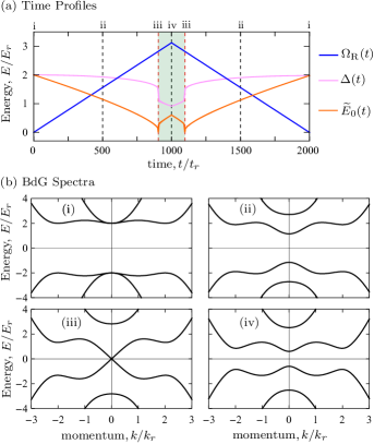
Figure 1: (a) Time profiles of $\Omega_{\mathrm{R}}(t)$, $\Delta(t)$, and $\widetilde{E}_{0}(t)$ for $t_{\mathrm{ramp}}=1000t_{r}$. The dashed lines denote the times whose instantaneous band diagrams are plotted in (b). The red dashed lines mark the critical times when TPT happens, and the shaded region corresponds to the topological regime. Plots are obtained from numerically solving the td-BdGE [Eq. (11)] self-consistently [Eqs. (12a) and  (12b)] with initial parameters: $\Omega_{\mathrm{R}}(0)=0$, $\Delta(0)=2E_{r}$ and $\mu(0)=0$ for SOC strength $\alpha=2E_{r}/k_{r}$ and $t_{\mathrm{ramp}}=1000t_{r}$. (b) Quasiparticle spectra at different Zeeman potentials $\Omega_{\mathrm{R}}$. From top to bottom, the energy bands are labeled by $E_{2,k},E_{1,k},E_{-1,k}$, and $E_{-2,k}$. The parameters are as follows: (i) $\Omega_{\mathrm{R}}=0$, $\Delta=2E_{r}$, $\mu=0$, (ii) $\Omega_{\mathrm{R}}=1.56E_{r}$, $\Delta=1.93E_{r}$, $\mu=-0.02E_{r}$, (iii) $\Omega_{\mathrm{R}}=2.8E_{r}$, $\Delta=1.4E_{r}$, $\mu=-0.14E_{r}$, and (iv) $\Omega_{\mathrm{R}}=3.12E_{r}$, $\Delta=0.91E_{r}$, $\mu=-0.3E_{r}$.

The system’s Hamiltonian in the Nambu basis $\Psi_{k}(t)=(\psi_{k\uparrow}(t),\psi_{k\downarrow}(t),\psi^{\dagger}_{-k\downarrow}(t),-\psi^{\dagger}_{-k\uparrow}(t))^{\top}$ is $H(t)=\frac{1}{2}\int dk\Psi_{k}(t)^{\dagger}\mathcal{H}_{\mathrm{BdG},k}(t)\Psi_{k}(t)$, where $\psi_{k\sigma}(\psi^{\dagger}_{k\sigma})$ denote the annihilation (creation) operators for fermions with momentum $k$ and spin $\sigma$. The Bogoliubov–de Gennes (BdG) Hamiltonian is roman ; oreg ; Wei ; sau1

$$\mathcal{H}_{\mathrm{BdG},k}(t)=\xi_{k}(t)\tau_{z}+\alpha k\tau_{z}\sigma_{z}+\frac{\Omega_{\mathrm{R}}(t)}{2}\sigma_{x}+\Delta(t)\tau_{x},$$ (1)

where $\boldsymbol{\sigma}$ and $\boldsymbol{\tau}$ are vectors of Pauli operators acting on spin and particle-hole space, respectively. Here, $\xi_{k}(t)=\hbar^{2}k^{2}/2m-\mu(t)$ combines the kinetic energy and the chemical potential $\mu(t)$, which is determined self-consistently to keep the number of atoms fixed.

The mean-field pairing potential

$$\Delta(t)e^{i\vartheta(t)}=g_{\mathrm{1D}}\int{\langle\psi_{k\uparrow}(t)\psi_{-k\downarrow}(t)\rangle dk}$$ (2)

is also self-consistently determined, where $\langle\dots\rangle$ denotes averaging with respect to the initial thermal distribution. The attractive effective 1D coupling constant $g_{\mathrm{1D}}<0$ can be controlled by Feshbach tuning the three-dimensional (3D) scattering length bergeman ; astra ; liu . In Eq. (1), we used the transformed basis where $\psi_{k\sigma}(t)\rightarrow\psi_{k\sigma}(t)\exp[i\vartheta(t)/2]$, giving a real pairing potential: $\Delta(t)\exp[i\vartheta(t)]\rightarrow\Delta(t)$.

The instantaneous quasiparticle excitation spectrum of the BdG Hamiltonian [cf. Fig. 1(b)] consists of four bands, $E_{n,k}=\operatorname{sgn}(n)\epsilon_{(-1)^{n},k}$, where $n=\pm 1,\pm 2$ and

$$\epsilon^{2}_{\pm,k}(t) = \frac{\Omega_{\mathrm{R}}(t)^{2}}{4}+\Delta(t)^{2}+\xi_{k}(t)^{2}+\alpha^{2}k^{2}$$

$$\pm 2\sqrt{\xi_{k}(t)^{2}\left[\alpha^{2}k^{2}+\frac{\Omega_{\mathrm{R}}(t)^{2}}{4}\right]+\Delta(t)^{2}\frac{\Omega_{\mathrm{R}}(t)^{2}}{4}}.\$$

Since $\mathcal{H}_{\mathrm{BdG},k}$ respects particle-hole symmetry, the spectrum is symmetric around $E=0$. As shown in Fig. 1(b), the instantaneous energy spectrum is gapped for $k\neq 0$; however, for $k=0$ the gap closes when $\epsilon_{-,0}(t)=\Omega_{\mathrm{R}}(t)/2-\sqrt{\Delta(t)^{2}+\mu(t)^{2}}=0$. Such a gap closing without change in the symmetry of the ground state (which remains SF for all $\Omega_{\mathrm{R}}$) signifies a TPT roman ; jay2 ; oreg between topological $[\epsilon_{-,0}(t)>0]$ and conventional SF phases $[\epsilon_{-,0}(t)<0]$. For $\Omega_{\mathrm{R}}=0$, the positive and negative bands are doubly degenerate at $k=0$; any nonzero $\Omega_{\mathrm{R}}$ lifts this degeneracy.

To study the dynamics around the TPT, we propose to prepare conventional SFs $[\epsilon_{-,0}(t)<0]$ at nonzero temperature $T$. We then drive the system through the TPT by changing $\Omega_{\mathrm{R}}$ according to our ramp protocol with $\Omega_{\mathrm{R}f}>2\sqrt{\Delta_{f}^{2}+\mu_{f}^{2}}$ (where the subscript $f$ denotes the quantities at time $t=t_{\mathrm{ramp}}$) such that the ramp crosses the TPT (cf. Fig. 1).

We first analytically study the dynamics, considering the simple case of slow ramps at $T=0$. In this limit, excitations occur near $k=0$ and at the transition times $t=t_{c(1,2)}$, given by the roots of $\Omega_{\mathrm{R}}(t_{c})=2\sqrt{\Delta(t_{c})^{2}+\mu(t_{c})^{2}}$, where the Fermi gas changes from conventional to TSF and vice versa. For $\hbar^{2}k^{2}/2m\ll\alpha k$, we approximate

$$\mathcal{H}_{\mathrm{BdG},k}(t)\approx\alpha k\tau_{z}\sigma_{z}-\mu(t)\tau_{z}+\frac{\Omega_{\mathrm{R}}(t)}{2}\sigma_{x}+\Delta(t)\tau_{x}.$$ (4)

In this limit, excitations occur only between the $E_{1,k}$ and $E_{-1,k}$ bands [cf. Fig. 1(b)]. At $k=0$, the eigenenergies are $\pm\widetilde{E}_{0}(t)$, where $\widetilde{E}_{0}(t)=|\sqrt{\Delta(t)^{2}+\mu(t)^{2}}-\Omega_{\mathrm{R}}(t)/2|$ with eigenstates

$$\widetilde{\phi}_{0}^{+}(t) =\left(\begin{matrix}\cos\frac{\theta(t)}{2}\\ \sin\frac{\theta(t)}{2}\end{matrix}\right)\otimes\frac{1}{\sqrt{2}}\left(\begin{matrix}1\\ 1\end{matrix}\right),$$ (5a)

$$\widetilde{\phi}_{0}^{-}(t) =\left(\begin{matrix}-\sin\frac{\theta(t)}{2}\\ \cos\frac{\theta(t)}{2}\end{matrix}\right)\otimes\frac{1}{\sqrt{2}}\left(\begin{matrix}1\\ -1\end{matrix}\right),$$ (5b)

where $\widetilde{\phi}_{0}^{\pm}(t)$ corresponds to positive and negative bands [with pseudospin $\left|\pm\right\rangle\equiv(\left|\uparrow\right\rangle\pm\left|\downarrow\right\rangle)/\sqrt{2}$] and $\cos\theta(t)\equiv\mu(t)/\sqrt{\Delta(t)^{2}+\mu(t)^{2}}$. In the subspace of these eigenstates, the effective low-energy Hamiltonian near $k=0$ is

$$\widetilde{\mathcal{H}}_{\mathrm{BdG},k}(t) = \widetilde{\alpha}(t)k\eta_{x}+\widetilde{E}_{0}(t)\eta_{z},$$ (6)

where $\widetilde{\alpha}(t)=\alpha\sin\theta(t)$, $\eta_{x}=\widetilde{\phi}_{0}^{+}(t)[\widetilde{\phi}_{0}^{-}(t)]^{\dagger}+\mathrm{H.c.}$, $\eta_{z}=\widetilde{\phi}_{0}^{+}(t)[\widetilde{\phi}_{0}^{+}(t)]^{\dagger}-\widetilde{\phi}_{0}^{-}(t)[\widetilde{\phi}_{0}^{-}(t)]^{\dagger}$, and $2\eta_{y}=-i[\eta_{z},\eta_{x}]$. Equation (6) is a two-parameter driven Hamiltonian sau1 with instantaneous energy eigenvalues $\pm\widetilde{E}_{k}(t)$, where $\widetilde{E}_{k}(t)=\sqrt{\widetilde{E}_{0}(t)^{2}+\widetilde{\alpha}(t)^{2}k^{2}}$.

We analyze the dynamics of the TPT using $\widetilde{\mathcal{H}}_{\mathrm{BdG},k}(t)$, where the single-particle state of the system at time $t$ is given by

$$\widetilde{\phi}_{k}(t)=b_{k}^{+}(t)\left(\begin{matrix}w^{+}_{k}(t)\\ \operatorname{sgn}(k)w^{-}_{k}(t)\end{matrix}\right)+b_{k}^{-}(t)\left(\begin{matrix}-\operatorname{sgn}(k)w^{-}_{k}(t)\\ w^{+}_{k}(t)\end{matrix}\right),$$ (7)

with the initial conditions $b_{k}^{+}(0)=0$ and $b_{k}^{-}(0)=1$. These two-component vectors are expressed in the basis $\widetilde{\phi}_{0}^{\pm}$ with $w^{\pm}_{k}(t)=\sqrt{[1\pm\widetilde{E}_{0}(t)/\widetilde{E}_{k}(t)]/2}$. The Schrödinger equation for the system then leads to

$$i\hbar\partial_{t}\vec{b}_{k}(t)=\widetilde{\mathcal{H}}_{\mathrm{BdG},k}(t)\vec{b}_{k}(t),$$ (8)

where $\vec{b}_{k}(t)=(b_{k}^{+}(t),b_{k}^{-}(t))^{\top}$.

We make further analytical progress by ignoring the self-consistency condition so that the system can be treated as a collection of two-level systems for each $(k,-k)$ pair and use the adiabatic-impulse approximation damski05 ; damski06 ; nori ; adutt1 ; Dziarmaga ; note that describes such periodic dynamics accurately for low frequency and/or large amplitude drives. Within this approximation, excitations are produced only near the critical gap-closing times $t_{c(1,2)}$ when the system enters the impulse regime; otherwise, the dynamics occur adiabatically in each band and the system accumulates a dynamical phase $U(t_{f},t_{i})=\exp[-i\eta_{z}\int_{t_{i}}^{t_{f}}{dt\widetilde{E}_{k}(t)/\hbar}]$. In the former regime, near the gap-closing times $t_{c(1,2)}$, excitations are produced and the evolution operator is nori

$$N=\sqrt{1-p_{k}}[i\sin(\varphi_{\mathrm{S},k})-\eta_{z}\cos(\varphi_{\mathrm{S},k})]-i\eta_{y}\sqrt{p_{k}},$$ (9)

where $p_{k}=\exp\left({-2\pi\delta_{k}}\right)$ is the probability of excitation formation in each passage through the critical point landau ; zener with $\delta_{k}=(\alpha k)^{2}/(2\hbar|d\widetilde{E}_{0}(t)/dt|_{t_{c}})$, and $\varphi_{\mathrm{S},k}=\pi/4+\delta_{k}(\ln\delta_{k}-1)+\arg\Gamma(1-i\delta_{k})$ is the Stokes phase originating from the interference of the parts of the system wave function in the instantaneous ground and excited states at $t=t_{c(1,2)}$ with $\arg\Gamma(1-i\delta_{k})$ being the argument of the gamma function gradshteyn . These results give the probability of defect formation

$$P^{\mathrm{ex}}_{k}=4p_{k}(1-p_{k})\sin^{2}\Phi_{\mathrm{St},k}$$ (10)

at $t=2t_{\mathrm{ramp}}$, where $\Phi_{\mathrm{St},k}=\zeta_{2k}+\varphi_{\mathrm{S},k}$ is the Stückelberg phase and $\zeta_{2k}=\int_{t_{c1}}^{t_{c2}}dt\widetilde{E}_{k}(t)/\hbar$ is the dynamical phase factor accumulated during passage between the two crossings of the gap-closing points nori ; adutt1 ; note . Since the excitations occur near $k\sim 0$ where the $E_{\pm 1,k}$ band approximately corresponds to pseudospin $|\pm\rangle$ (along the $x$ direction), $P^{\mathrm{ex}}_{k}$ is directly related to changes in the SRMD $\delta n_{k\pm}$ measured along the pseudospin $x$ direction. Furthermore, within these approximations, $|d\widetilde{E}_{0}(t)/dt|_{t_{c(1,2)}}=\Omega_{\mathrm{R}f}/(2t_{\mathrm{ramp}})$, and it can be shown that $P_{k}^{\mathrm{ex}}$ is a function of $k\sqrt{t_{\mathrm{ramp}}}$ only (see Ref. note for the derivation). Thus, the integrated change of the SRMD $\delta{\widetilde{n}}_{\pm}=\int dk\delta n_{k\pm}$ displays KZ scaling $\sim\sqrt{t_{\rm ramp}}$ of defect density for a system dynamically evolved through the TPT. We now show that these properties persist even when the self-consistency conditions for $\Delta(t)$ and $\mu(t)$ are imposed, as well as at nonzero $T$ (see Fig. 2).

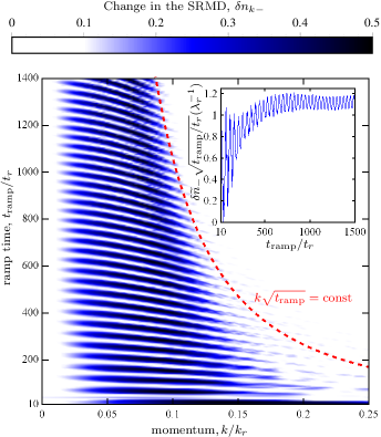
Figure 2: Change in the SRMD $\delta n_{k-}$ for spin $\left|-\right\rangle=\left(\left|\uparrow\right\rangle-\left|\downarrow\right\rangle\right)/\sqrt{2}$ as a function of $t_{\rm ramp}/t_{r}$ and $k/k_{r}$. For large $t_{\rm ramp}$, the width of the oscillation envelopes scales with $1/\sqrt{t_{\mathrm{ramp}}}$ as shown by the red dashed line. $\delta n_{k-}$ is symmetric with respect to $k=0$; thus, for illustration purposes, we only plot $\delta n_{k-}$ for $k\geq 0$. Note that $\delta n_{k+}=-\delta n_{k-}$. Inset: Integrated change in SRMD $\delta\widetilde{n}_{-}=\int{dk\delta n_{k-}}$ as a function of $t_{\rm ramp}/t_{r}$ exhibiting oscillations, with the amplitude of the oscillations at large $t_{\rm ramp}$ scaling like $\sqrt{t_{\rm ramp}}$, as can be read off directly from the $y$ axis. The plots are obtained by numerically solving Eq. (11) self-consistently [Eqs. (12a) and (12b)] with initial conditions $\mu(0)=0$, $\Delta(0)=2E_{r}$, and $\Omega_{\mathrm{R}}(0)=0$ for a temperature $k_{\mathrm{B}}T=0.1E_{\mathrm{F}}$ (which is below the critical temperature $T_{c}=0.19T_{\mathrm{F}}$ Nascimbene ; Zwierlein ), SOC strength $\alpha=2E_{r}/k_{r}$, and $\Omega_{\mathrm{R}f}=3.12E_{r}$.

We solve for the dynamics of the single-particle density matrix $\rho^{ab}_{k}(t)=\langle\Psi^{\dagger a}_{k}(t)\Psi^{b}_{k}(t)\rangle$ self-consistently and at finite initial temperature, where $a,b$ denote the indices of elements in the Nambu basis. The density matrix obeys the equation of motion [Eq. (1)]

$$i\hbar\partial_{t}\rho_{k}(t)=[\mathcal{H}_{\mathrm{BdG},k}(t),\rho_{k}(t)],$$ (11)

subject to the self-consistency conditions (see Ref. note for the derivation)

$$\Delta(t) =\frac{g_{\mathrm{1D}}}{4}\int{dk\mathrm{Tr}(\rho_{k}(t)\tau_{x})},$$ (12a)

$$\mu(t) =\frac{g_{\mathrm{1D}}}{4\Delta(t)}\int dk\mathrm{Tr}\left(\rho_{k}(t)\Lambda_{k}(t)\right),$$ (12b)

where $\Lambda_{k}(t)=\left(\hbar^{2}k^{2}/2m+\alpha k\sigma_{z}\right)\tau_{x}-\Delta(t)\tau_{z}$. Our system begins in the thermal state

$$\rho_{k}(t)=\sum_{\begin{subarray}{c}n\\ E_{n,k}(0)<0\end{subarray}}f_{n,k}\chi_{n,k}(t)\chi_{n,k}^{\dagger}(t)+(1-f_{n,k})\widetilde{\chi}_{n,-k}(t)\widetilde{\chi}_{n,-k}^{\dagger}(t),$$ (13)

where $f_{n,k}=[\exp(E_{n,k}(0)/k_{\mathrm{B}}T)+1]^{-1}$ is the Fermi function of the initial Hamiltonian, and $k_{\mathrm{B}}$ is Boltzmann’s constant. The wave function $\chi_{n,k}(t)$ with its particle-hole conjugate $\widetilde{\chi}_{n,k}(t)=\tau_{y}\sigma_{y}\chi_{-n,-k}^{\ast}(t)$ begins as eigenfunctions of the initial Hamiltonian and evolves according to $i\hbar\partial_{t}\chi_{n,k}(t)=\mathcal{H}_{\mathrm{BdG},k}(t)\chi_{n,k}(t)$. Figure 1(a) shows the resulting time profiles of the pairing potential obtained from solving the td-BdGE (see Ref. note for the time dependence of all parameters and remarks on the numerical simulation).

We numerically solved the td-BdGE for the change in the SRMD

$$\delta n_{k\pm}=\mathrm{Tr}\left(\left[\rho_{k}(2t_{\mathrm{ramp}})-\rho_{k}(0)\right]\left[\left(\frac{1+\tau_{z}}{2}\right)\otimes\left(\frac{1\pm\sigma_{x}}{2}\right)\right]\right).$$ (14)

Figure 2 shows that $\delta n_{k-}$ still exhibits Stückelberg oscillations even with inclusion of the self-consistency conditions and at $T>0$. Furthermore, for $t_{\mathrm{ramp}}\gg\hbar/\Delta_{f}$, we still see $\delta{n}_{k\pm}\sim k\sqrt{t_{\rm ramp}}$ (see Ref. note for an explicit demonstration of the scaling), and the integrated change in SRMD $\delta{\widetilde{n}}_{\pm}=\int dk\delta{n}_{k\pm}$ therefore scales with $\sqrt{t_{\mathrm{ramp}}}$, thus, showing the robustness of such interference phenomenon in the present system. We verified that these features appear only if $\Omega_{\mathrm{R}f}>2\sqrt{\Delta_{f}^{2}+\mu_{f}^{2}}$, where the ramp takes the system through the TPT; thus both the KZ scaling and the presence of Stückelberg oscillations mark the TPT. In our calculation, we ignored the effect of phase fluctuation as this effect can be suppressed by coupling an array of 1D SOCFGs mizushima ; sau2 ; meng ; fidkowski .

The parameters used for the plots in Fig. 2 are realistic for 1D SOCFG experiments. For experiments with ⁴⁰K, the Raman laser beams, coupling the $\left|\uparrow\right\rangle\equiv\left|9/2,-7/2\right\rangle$ and $\left|\downarrow\right\rangle\equiv\left|9/2,-9/2\right\rangle$ states, have laser wavelength $\lambda_{r}=768.86$ nm, giving the recoil energy $E_{r}=h\times 8.445$ kHz, and time $t_{r}=\hbar/E_{r}\approx 20$ $\mu$s Williams13 . The single-body decay time due to photons scattering from the Raman lasers is about 60 ms Williams13 , and the lifetime owing to three-body recombination is about 200 ms Jin04 . We consider SOCFGs with Fermi energy $E_{\mathrm{F}}=E_{r}$. The 1D Fermi gas criterion is satisfied when $E_{\mathrm{F}}<\hbar\omega_{\perp}$; for the lateral trapping frequency $\omega_{\perp}/2\pi=5\times 10^{4}$ Hz, which corresponds to characteristic harmonic oscillator length $d_{\perp}=\sqrt{\hbar/m\omega_{\perp}}\approx 1345a_{0}$, where $a_{0}$ is the Bohr radius; the parameters used in the calculation for the plots in Fig. 2 correspond to linear density $\widetilde{n}\approx 5$ $\mu\mathrm{m}^{-1}$ and 1D interaction strength $g_{\mathrm{1D}}\approx-0.73E_{r}\lambda_{r}$ (or 3D scattering length $a_{\mathrm{3D}}\approx-2870a_{0}$ liu ). For these values, Fig. 2 shows that the Stückelberg oscillations and KZ scaling behavior of the SRMD can be observed within the experimentally limiting single-body decay time $(\approx 3000t_{r})$ and thus is feasible experimentally.

Our dip-in-dip-out protocol is quite general and can be gainfully used for observing features related to quantum phase transitions between long-lived and short-lived phases of ultracold bosonic and fermionic atoms. In addition, it provides a route to escaping the heating problem, which is one of the major obstacles in measuring properties of such systems in or near their short-lived phases. Moreover, our work also shows that such a protocol applied to ultracold atom systems, including the one we analyzed in detail, may provide us with test beds for observation of both KZ scaling Sadler ; Weiler ; Lamporesi ; Chen ; Navon ; Braun ; Corman ; Chomaz and Stückelberg interference phenomenon Mark ; Kling ; Zenesini .

We thank H.-Y. Hui, S. S. Natu, and J. Radić for useful discussions. F. S. and J. D. S. acknowledge the support from LPS-CMTC, JQI-NSF-PFC and University of Maryland startup grants. I. B. S. gratefully acknowledges funding from the ARO’s Atomtronics-MURI, the AFOSR’s quantum matter MURI, the NSF through the JQI Physics Frontier Center, and NIST.

Supplemental Material for “Dynamical Detection of Topological Phase Transitions in Short-Lived Atomic Systems”

I Adiabatic-Impulse Approximation

The equation of motion $i\hbar\partial_{t}\vec{b}_{k}(t)=\widetilde{\mathcal{H}}_{\mathrm{BdG},k}(t)\vec{b}_{k}(t)$ [Eq. (8)], where $\vec{b}_{k}(t)=(b_{k}^{+}(t),b_{k}^{-}(t))^{\top}$ [Eq. (7)] and $\widetilde{\mathcal{H}}_{\mathrm{BdG},k}(t)=\widetilde{\alpha}(t)k\eta_{x}+\widetilde{E}_{0}(t)\eta_{z}$ [Eq. (6)] with $\eta_{x}$ and $\eta_{z}$ being the Pauli matrices acting on the subspace $\widetilde{\phi}_{0}^{\pm}(t)$ [Eq. (5)], can be expressed in form of two-decoupled second-order differential equations as

$$\left\{-\hbar^{2}\partial_{t}^{2}-\widetilde{E}_{k}(t)^{2}+i\hbar\left[\mp\partial_{t}\widetilde{E}_{0}(t)\pm\widetilde{E}_{0}(t)\partial_{t}-\frac{\partial_{t}\widetilde{\alpha}(t)}{\widetilde{\alpha}(t)}\left[i\hbar\partial_{t}\mp\widetilde{E}_{0}(t)\right]\right]\right\}b_{k}^{\pm} =0.$$ (S-1)

Assuming no self-consistency, we can use the adiabatic-impulse approximation nori to write Eq. (S-1) as $\vec{b}_{k}(t)=V\vec{b}_{k}(0)$ where the total evolution operator $V$ is decomposed into adiabatic $U$ and impulse $N$ operators. The adiabatic (impulse) regime corresponds to the time duration far away from (near) the critical gap-closing time $t_{c(1,2)}$. In matrix form we can write down $U$ as

$$U_{j}=\left(\begin{matrix}e^{-i\zeta_{jk}}&0\\ 0&e^{i\zeta_{jk}}\end{matrix}\right),\hskip 8.5359ptj=1,2,3,$$ (S-2)

where the dynamical phases are given by $\zeta_{1k}=\int_{0}^{t_{c1}}{dt\widetilde{E}_{k}(t)/\hbar}$, $\zeta_{2k}=\int_{t_{c1}}^{t_{c2}}{dt\widetilde{E}_{k}(t)/\hbar}$, and $\zeta_{3k}=\int_{t_{c2}}^{2t_{\mathrm{ramp}}}{dt\widetilde{E}_{k}(t)/\hbar}$. The impulse operator $N$ can be written as nori

$$\hskip 8.5359pt\hskip 14.22636ptN=\left(\begin{matrix}\sqrt{1-p_{k}}e^{-i\widetilde{\varphi}_{\mathrm{S},k}}&-\sqrt{p_{k}}\\ \sqrt{p_{k}}&\sqrt{1-p_{k}}e^{i\widetilde{\varphi}_{\mathrm{S},k}}\end{matrix}\right),$$ (S-3)

where $p_{k}=\exp(2\pi\delta_{k})$ is the landau-Zener transition probability landau ; zener at each critical time, $\delta_{k}=(\alpha k)^{2}/(2\hbar|d\widetilde{E}_{0}(t)/dt|_{t_{c}})$, $\widetilde{\varphi}_{\mathrm{S},k}=\varphi_{\mathrm{S},k}-\pi/2$ and $\varphi_{\mathrm{S},k}=\pi/4+\delta_{k}(\ln\delta_{k}-1)+\arg\Gamma(1-i\delta_{k})$. The Stokes phase $\varphi_{\mathrm{S},k}$ increases monotonously from $0$ in the adiabatic limit ($\delta_{k}\rightarrow\infty$) to $\pi/4$ in the diabatic or fast driving limit ($\delta_{k}\rightarrow 0$), as seen from the asymptotic argument of the gamma function gradshteyn

$$\mathrm{arg}~{}\Gamma(1-i\delta_{k})\approx\begin{cases}C\delta_{k},&\delta_{k}\ll 1,\\ -\frac{\pi}{4}-\delta_{k}(\ln\delta_{k}-1),&\delta_{k}\gg 1,\end{cases}$$ (S-4)

where $C\approx 0.58$ is the Euler constant. At the end of the ramp protocol, the total evolution operator becomes

$$V=U_{3}NU_{2}NU_{1}=\left(\begin{matrix}\beta_{k}&-\gamma_{k}^{*}\\ \gamma_{k}&\beta_{k}^{*}\end{matrix}\right),$$ (S-5)

with matrix elements

$$\beta_{k} =(1-p_{k})e^{-i\zeta_{+k}}-p_{k}e^{-i\zeta_{-k}},$$

$$\gamma_{k} =\sqrt{(1-p_{k})p_{k}}e^{i(\widetilde{\varphi}_{\mathrm{S},k}+2\zeta_{3k})}\left(e^{-i\zeta_{+k}}+e^{-i\zeta_{-k}}\right),$$ (S-6)

where the phases are given by $\zeta_{+k}=\zeta_{1k}+\zeta_{2k}+\zeta_{3k}+2\widetilde{\varphi}_{\mathrm{S},k}$ and $\zeta_{-k}=\zeta_{1k}-\zeta_{2k}+\zeta_{3k}$. The probability of defect formation at the end of the ramp protocol (at $t=2t_{\mathrm{ramp}}$) is then given by

$$P^{\mathrm{ex}}_{k}=|\gamma_{k}|^{2}=4p_{k}(1-p_{k})\sin^{2}\Phi_{\mathrm{St},k},$$ (S-7)

where $\Phi_{\mathrm{St},k}=\zeta_{2k}+\varphi_{\mathrm{S},k}$ is the Stückelberg phase. Note that in the case of no-self consistency, $|d\widetilde{E}_{0}(t)/dt|=\Omega_{\mathrm{R}f}/(2t_{\mathrm{ramp}})$, and consequently $\delta_{k}$ is a function of $k\sqrt{t_{\mathrm{ramp}}}$. Since $p_{k}$ and $\varphi_{\mathrm{S},k}$ are functions of $\delta_{k}$, $P^{\mathrm{ex}}_{k}$ is also a function of $k\sqrt{t_{\mathrm{ramp}}}$. As a result, the defect density displays Kibble-Zurek scaling $\sim\sqrt{t_{\mathrm{ramp}}}$.

II Self-Consistency Condition

The self-consistent chemical potential $\mu(t)$ [Eq. (12b)] is derived from the constraint on the particle density $\widetilde{n}$, i.e.,

$$\int dk\mathrm{Tr}\left(\rho_{k}(t)\left(\frac{1+\tau_{z}}{2}\right)\right)=\widetilde{n}.$$ (S-8)

Taking the time derivative of Eq. (S-8), i.e., $i\hbar\partial_{t}\rho_{k}(t)=[\mathcal{H}_{\mathrm{BdG},k}(t),\rho_{k}(t)]$, and using the cyclic property of trace, we have

$$\frac{1}{2}\int{dk\mathrm{Tr}([\mathcal{H}_{\mathrm{BdG},k}(t),\rho_{k}(t)]\tau_{z})} =0$$

$$\frac{1}{2}\int{dk\mathrm{Tr}([\tau_{z},\mathcal{H}_{\mathrm{BdG},k}(t)]\rho_{k}(t))} =0$$

$$\int{dk\mathrm{Tr}(\tau_{y}\rho_{k}(t))} =0.$$ (S-9)

Differentiating Eq. (II) with respect to time and using the cyclic property of trace, we then obtain

$$\int{dk\mathrm{Tr}(\tau_{y}[\mathcal{H}_{\mathrm{BdG},k}(t),\rho_{k}(t)])} =0$$

$$\int{dk\mathrm{Tr}([\mathcal{H}_{\mathrm{BdG},k}(t),\tau_{y}]\rho_{k}(t))} =0$$

$$\int{dk\mathrm{Tr}\left((\hbar^{2}k^{2}/2m-\mu(t)+\alpha k\sigma_{z})\tau_{x}\rho_{k}(t)-\Delta(t)\tau_{z}\rho_{k}(t)\right)} =0.$$ (S-10)

Noting that $g_{\mathrm{1D}}\int{dk\mathrm{Tr}(\rho_{k}(t)\tau_{x})}/4=\Delta(t)$, we then have the self-consistent chemical potential $\mu(t)$ as

$$\mu(t)=\frac{g_{\mathrm{1D}}}{4\Delta(t)}\int{dk\mathrm{Tr}\left((\hbar^{2}k^{2}/2m+\alpha k\sigma_{z})\tau_{x}\rho_{k}(t)-\Delta(t)\tau_{z}\rho_{k}(t)\right)}.$$ (S-11)

III Remarks on The Numerical Simulation

In the main text, the td-BdGE is given in terms of the single-particle density matrix $\rho_{k}(t)$. The td-BdGE can also be written in terms of the wave function $\chi_{n,k}(t)=(u_{n,k\uparrow}(t),u_{n,k\downarrow}(t),v_{n,k\downarrow}(t),-v_{n,k\uparrow}(t))^{\top}$ as

$$i\hbar\partial_{t}\chi_{n,k}(t)=\mathcal{H}_{\mathrm{BdG},k}(t)\chi_{n,k}(t),$$ (S-12)

subject to the self-consistency conditions

$$\Delta(t) =\frac{g_{\mathrm{1D}}}{4}\sum_{\begin{subarray}{c}n\\ E_{n,k}(0)<0\end{subarray}}\int dk\mathcal{I}^{-}_{n,k}(t),$$ (S-13a)

$$\mu(t) =\frac{g_{\mathrm{1D}}}{4\Delta(t)}\sum_{\begin{subarray}{c}n\\ E_{n,k}(0)<0\end{subarray}}\int dk\left[\frac{\hbar^{2}k^{2}}{2m}\mathcal{I}^{-}_{n,k}(t)+\alpha k\mathcal{I}^{+}_{n,k}(t)-\Delta(t)\mathcal{Q}_{n,k}(t)\right],$$ (S-13b)

where

$$\mathcal{I}_{n,k}^{\pm}(t) =(2f_{n,k}-1)\{[v^{*}_{n,k\downarrow}(t)u_{n,k\uparrow}(t)\pm u_{n,k\downarrow}(t)v^{*}_{n,k\uparrow}(t)]+\mathrm{H.c.}\},$$ (S-14a)

$$\hskip 8.5359pt\mathcal{Q}_{n,k}(t) =(2f_{n,k}-1)\sum_{\sigma}(|u_{n,k\sigma}|^{2}-|v_{n,k\sigma}|^{2}),$$ (S-14b)

with $f_{n,k}=[\exp(E_{n,k}(0)/k_{\mathrm{B}}T)+1]^{-1}$ being the Fermi function of the initial Hamiltonian.

The self-consistent solution of the td-BdGE involves solving a large number of coupled time-dependent differential equations (one for each $k$ point). To reduce the number of time-dependent variables, we first calculated the self-consistent $\Delta(t)$ and $\mu(t)$ in the adiabatic regime by solving the time-independent BdG equation. The td-BdGE was then solved self-consistently for a small range of states near $k=0$ where excitations occur. Since the $\pm k$ eigenstates are related by $\mathrm{X}_{n,-k}=\sigma_{x}\mathrm{X}_{n,k}$, we accelerated the computation by focusing on $k\geq 0$. Solving the td-BdGE self-consistently with the Zeeman potential $\Omega_{\mathrm{R}}(t)$ varied according the piecewise linear ramp protocol (see blue curve in Fig. S1), we obtained $\widetilde{\alpha}(t)$, $\Delta(t)$, $\widetilde{E}_{0}(t)$, and $\mu(t)$ as shown in Fig. S1.

Supplementary Figure S1: Time profiles of $\Omega_{\mathrm{R}}(t)$, $\widetilde{\alpha}(t)$, $\Delta(t)$, $\widetilde{E}_{0}(t)$ and $\mu(t)$ for $t_{\mathrm{ramp}}=1000t_{r}$. The dashed lines denote the times whose instantaneous band diagrams are plotted in Fig. 1(b) in the main text. The red dashed lines mark the critical times when TPT happens, and the shaded region corresponds to the topological regime. Plots are obtained from numerically solving the td-BdGE self-consistently with initial parameters: $\Omega_{\mathrm{R}}(0)=0$, $\Delta(0)=2E_{r}$, and $\mu(0)=0$ for SOC strength $\alpha=2E_{r}/k_{r}$ and $t_{\mathrm{ramp}}=1000t_{r}$.

IV Spin-Resolved Momentum Distribution

The change in spin-resolved momentum distribution $\delta n_{k-}$ shows Stückelberg oscillations with the ramp time $t_{\mathrm{ramp}}$ and for large $t_{\mathrm{ramp}}$, $\delta n_{k-}$ scales with $\sqrt{t_{\mathrm{ramp}}}$, as shown in Fig. 2 in the main text. In Fig. S2, we demonstrate the scaling more explicitly by plotting $\delta n_{k-}$ as a function of scaled momentum $k/k_{r}\sqrt{t_{\rm ramp}/t_{r}}$.

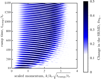
Supplementary Figure S2: Change in the SRMD $\delta n_{k-}$ for pseudospin $\left|-\right\rangle=\left(\left|\uparrow\right\rangle-\left|\downarrow\right\rangle\right)/\sqrt{2}$ as a function of $t_{\rm ramp}/t_{r}$ and $k/k_{r}\sqrt{t_{\rm ramp}/t_{r}}$. Note that $\delta n_{k-}$ is a function of $k\sqrt{t_{\rm ramp}}$ only for large $t_{\rm ramp}$, as seen from its almost flat nature for small $k/k_{r}$ and the width of its oscillation envelopes. The scaling of $\delta n_{k-}$ can be read off directly from the $x$ axis. $\delta n_{k-}$ is symmetric with respect to $k=0$; thus, for illustration purposes, we only plot $\delta n_{k-}$ for $k\geq 0$. The plots are obtained by numerically solving the td-BdGE self-consistently with initial conditions $\Omega_{\mathrm{R}}(0)=0$, $\Delta(0)=2E_{r}$ and $\mu(0)=0$ for a temperature $k_{\mathrm{B}}T=0.1E_{\mathrm{F}}$ (which is below the critical temperature $T_{c}=0.19T_{\mathrm{F}}$ Nascimbene ; Zwierlein ), SOC strength $\alpha=2E_{r}/k_{r}$, and $\Omega_{\mathrm{R}f}=3.12E_{r}$. Note that $\delta n_{k+}=-\delta n_{k-}$ due to particle number conservation.

References

(1) D. Jaksch, C. Bruder, J. I. Cirac, C. W. Gardiner, and P. Zoller, Phys. Rev. Lett. 81, 3108 (1998).
(2) M. Greiner, O. Mandel, T. Esslinger, T. W. Hänsch, and I. Bloch, Nature (London) 415, 39 (2002).
(3) S. Fölling, A. Widera, T. Müller, F. Gerbier, and I. Bloch, Phys. Rev. Lett. 97, 060403 (2006).
(4) G. K. Campbell, J. Mun, M. Boyd, P. Medley, A. E. Leanhardt, L. G. Marcassa, D. E. Pritchard, and W. Ketterle, Science 313, 649 (2006).
(5) I. B. Spielman, W. D. Phillips, and J. V. Porto, Phys. Rev. Lett. 98, 080404 (2007).
(6) W. S. Bakr, A. Peng, M. E. Tai, R. Ma, J. Simon, J. I. Gillen, S. Fölling, L. Pollet, and M. Greiner, Science 329, 547 (2010).
(7) D. Greif, T. Uehlinger, G. Jotzu, L. Tarruell, and T. Esslinger, Science 340, 1307 (2013).
(8) R. A. Hart, P. M. Duarte, T.-L. Yang, X. Liu, T. Paiva, E. Khatami, R. T. Scalettar, N. Trivedi, D. A. Huse, and R. G. Hulet, Nature (London) 519, 211 (2015).
(9) Y.-J. Lin, K. Jiménez-García, and I. B. Spielman, Nature (London) 471, 83 (2011).
(10) P. Wang, Z.-Q. Yu, Z. Fu, J. Miao, L. Huang, S. Chai, H. Zhai, and J. Zhang, Phys. Rev. Lett. 109, 095301 (2012).
(11) L. W. Cheuk, A. T. Sommer, Z. Hadzibabic, T. Yefsah, W. S. Bakr, and M. W. Zwierlein, Phys. Rev. Lett. 109, 095302 (2012).
(12) J.-Y. Zhang, S.-C. Ji, Z. Chen, L. Zhang, Z.-D. Du, B. Yan, G.-S. Pan, B. Zhao, Y.-J. Deng, H. Zhai, S. Chen, and J.-W. Pan, Phys. Rev. Lett. 109, 115301 (2012).
(13) C. Qu, C. Hamner, M. Gong, C. Zhang, and P. Engels, Phys. Rev. A 88, 021604(R) (2013).
(14) B. Béri and N. R. Cooper, Phys. Rev. Lett. 107, 145301 (2011).
(15) N. Goldman, I. Satija, P. Nikolic, A. Bermudez, M. A. Martin-Delgado, M. Lewenstein, and I. B. Spielman, Phys. Rev. Lett. 105, 255302 (2010).
(16) L. Mazza, A. Bermudez, N. Goldman, M. Rizzi, M. A. Martin-Delgado and M. Lewenstein, New. J. Phys. 14, 015007 (2012).
(17) L. Jiang, T. Kitagawa, J. Alicea, A. R. Akhmerov, D. Pekker, G. Refael, J. I. Cirac, E. Demler, M. D. Lukin, and P. Zoller, Phys. Rev. Lett. 106, 220402 (2011).
(18) X.-J. Liu, L. Jiang, H. Pu, and H. Hu, Phys. Rev. A 85, 021603(R) (2012).
(19) R. Wei and E. J. Mueller, Phys. Rev. A 86, 063604 (2012).
(20) C. Zhang, S. Tewari, R. M. Lutchyn, and S. Das Sarma, Phys. Rev. Lett. 101, 160401 (2008).
(21) M. Sato, Y. Takahashi, and S. Fujimoto, Phys. Rev. Lett. 103, 020401 (2009).
(22) J. D. Sau, R. Sensarma, S. Powell, I. B. Spielman, and S. Das Sarma, Phys. Rev. B 83, 140510(R) (2011).
(23) N. R. Cooper and J. Dalibard, Phys. Rev. Lett. 110, 185301 (2013).
(24) L. D. Landau, Phys. Z. Sowjetunion 2, 46 (1932).
(25) G. Zener, Proc. R. Soc. London, Ser. A 137, 696 (1932).
(26) T. Kibble, J. Phys. Math. Gen. 9, 1387 (1976).
(27) W. H. Zurek, Nature (London) 317, 505 (1985).
(28) L. E. Sadler, J. M. Higbie, S. R. Leslie, M. Vengalattore, and D. M. Stamper-Kurn, Nature (London) 443, 312 (2006).
(29) C. N. Weiler, T. W. Neely, D. R. Scherer, A. S. Bradley, M. J. Davis, and B. P. Anderson, Nature (London) 455, 948 (2008).
(30) D. Chen, M. White, C. Borries, and B. DeMarco, Phys. Rev. Lett. 106, 235304 (2011).
(31) G. Lamporesi, S. Donadello, S. Serafini, F. Dalfovo, and G. Ferrari, Nat. Phys. 9, 656 (2013).
(32) L. Corman, L. Chomaz, T. Bienaimé, R. Desbuquois, C. Weitenberg, S. Nascimbène, J. Dalibard, and J. Beugnon, Phys. Rev. Lett. 113, 135302 (2014).
(33) N. Navon, A. L. Gaunt, R. P. Smith, and Z. Hadzibabic, Science 347, 167 (2015).
(34) S. Braun, M. Friesdorf, S. S. Hodgman, M. Schreiber, J. P. Ronzheimer, A. Riera, M. del Rey, I. Bloch, J. Eisert, and U. Schneider, Proc. Natl. Acad. Sci. U.S.A 112, 3641 (2015).
(35) L. Chomaz, L. Corman, T. Bienaimé, R. Desbuquois, C. Weitenberg, S. Nascimbène, J. Beugnon, and J. Dalibard, Nat. Commun. 6, 6162 (2015).
(36) E. C. G. Stückelberg, Helv. Phys. Acta 5, 369 (1932).
(37) S. N. Shevchenko, S. Ashhab, and F. Nori, Phys. Rep. 492, 1, (2010).
(38) M. Greiner, O. Mandel, T. W. Hänsch, and I. Bloch, Nature (London) 419, 51 (2002).
(39) S. Mondal, D. Pekker, and K. Sengupta, Europhys. Lett. 100, 60007 (2012).
(40) U. Divakaran and K. Sengupta, Phys. Rev. B 90, 184303 (2014).
(41) A. Bermudez, D. Patanè, L. Amico, and M. A. Martin-Delgado, Phys. Rev. Lett. 102, 135702 (2009).
(42) A. Bermudez, L. Amico, and M. A. Martin-Delgado, New J. Phys. 12, 055014 (2010).
(43) W. DeGottardi, D. Sen, and S. Vishveshwara, New J. Phys. 13, 065028 (2011).
(44) E. Perfetto, Phys. Rev. Lett. 110, 087001 (2013).
(45) A. Rajak and A. Dutta, Phys. Rev. E 89, 042125 (2014).
(46) G. Kells, D. Sen, J. K. Slingerland, and S. Vishveshwara, Phys. Rev. B 89, 235130 (2014).
(47) P. D. Sacramento, Phys. Rev. E 90, 032138 (2014).
(48) S. Hegde, V. Shivamoggi, S. Vishveshwara, and D. Sen, New J. Phys. 17, 053036 (2015).
(49) J. Alicea, Rep. Prog. Phys. 75, 076501 (2012).
(50) M. Leijnse and K. Flensberg, Semicond. Sci. Technol. 27, 124003 (2012).
(51) C. W. J. Beenakker, Annu. Rev. Condens. Matter Phys. 4, 113 (2013).
(52) T. D. Stanescu and S. Tewari, J. Phys. Condens. Matter 25, 233201 (2013).
(53) S. R. Elliott and M. Franz, Rev. Mod. Phys. 87, 137 (2015).
(54) J. D. Sau, S. Tewari, R. M. Lutchyn, T. Stanescu, and S. Das Sarma, Phys. Rev. B 82, 214509 (2010).
(55) S. Nascimbène, J. Phys. B 46, 134005 (2013).
(56) A. Kitaev, Phys. Usp. 44, 131 (2001).
(57) R. A. Williams, M. C. Beeler, L. J. LeBlanc, K. Jiménez-García, and I. B. Spielman, Phys. Rev. Lett. 111, 095301 (2013).
(58) M. Greiner, C. A. Regal , and D. S. Jin, Nature (London) 426, 537 (2003).
(59) R. M. Lutchyn, J. D. Sau, and S. Das Sarma, Phys. Rev. Lett. 105, 077001 (2010).
(60) Y. Oreg, G. Refael, and F. von Oppen, Phys. Rev. Lett. 105, 177002 (2010).
(61) J. D. Sau and K. Sengupta, Phys. Rev. B 90, 104306 (2014).
(62) T. Bergeman, M. G. Moore, and M. Olshanii, Phys. Rev. Lett. 91, 163201 (2003).
(63) G. E. Astrakharchik, D. Blume, S. Giorgini, and L. P. Pitaevskii, Phys. Rev. Lett. 93, 050402 (2004).
(64) X.-J. Liu, H. Hu, and P. D. Drummond, Phys. Rev. A 76, 043605 (2007).
(65) B. Damski, Phys. Rev. Lett. 95, 035701 (2005).
(66) B. Damski and W. H. Zurek, Phys. Rev. A 73, 063405 (2006).
(67) A. Dutta, A. Das, and K. Sengupta, Phys. Rev. E 92, 012104 (2015).
(68) J. Dziarmaga, Adv. in Phys. 59, 1063 (2010).
(69) See Supplemental Material for detailed calculations of the probability of defect formation within the adiabatic-impulse approximation, a derivation of the self-consistent chemical potential, remarks on the numerical simulation and an explicit demonstration of the KZ scaling.
(70) I. S. Gradshteyn and I. M. Ryzhik, Table of Integrals, Series, and Products, 7th ed. (Academic Press, New York, 2007).
(71) S. Nascimbène, N. Navon, K. J. Jiang, F. Chevy, and C. Salomon, Nature (London) 463, 1057 (2010).
(72) M. J. H. Ku, A. T. Sommer, L. W. Cheuk, and M. W. Zwierlein, Science 335, 563 (2012).
(73) M. Cheng and H.-H. Tu, Phys. Rev. B 84, 094503 (2011).
(74) J. D. Sau, B. I. Halperin, K. Flensberg, and S. Das Sarma, Phys. Rev. B 84, 144509 (2011).
(75) L. Fidkowski, R. M. Lutchyn, C. Nayak, and M. P. A. Fisher, Phys. Rev. B 84, 195436 (2011).
(76) T. Mizushima and M. Sato, New. J. Phys. 15, 075010 (2013).
(77) C. A. Regal, M. Greiner, and D. S. Jin, Phys. Rev. Lett. 92, 083201 (2004).
(78) M. Mark, T. Kraemer, P. Waldburger, J. Herbig, C. Chin, H.-C. Nägerl, and R. Grimm, Phys. Rev. Lett. 99, 113201 (2007).
(79) S. Kling, T. Salger, C. Grossert, and M. Weitz, Phys. Rev. Lett. 105, 215301 (2010).
(80) A. Zenesini, D. Ciampini, O. Morsch, and E. Arimondo, Phys. Rev. A 82, 065601 (2010).