Energy-momentum tensor on the lattice: non- perturbative renormalization in Yang–Mills theory
Abstract
We construct an energy-momentum tensor on the lattice which satisfies the appropriate Ward Identities (WIs) and has the right trace anomaly in the continuum limit. It is defined by imposing suitable WIs associated to the Poincaré invariance of the continuum theory. These relations come forth when the length of the box in the temporal direction is finite, and they take a particularly simple form if the coordinate and the periodicity axes are not aligned. We implement the method for the SU(3) Yang–Mills theory discretized with the standard Wilson action in presence of shifted boundary conditions in the (short) temporal direction. By carrying out extensive numerical simulations, the renormalization constants of the traceless components of the tensor are determined with a precision of roughly half a percent for values of the bare coupling constant in the range .
I Introduction
On the lattice the Poincaré group is explicitly broken into discrete subgroups, and the full symmetry is recovered only in the continuum limit. As a consequence, a given definition of the energy-momentum tensor needs to be properly renormalized to guarantee that the associated charges are the generators of the Poincaré group in the continuum limit, and that the trace anomaly is correctly reproduced.
In order to construct the renormalized energy-momentum tensor, the way to proceed is to impose suitable WIs at fixed lattice spacing that hold up to cutoff effects which vanish in the continuum limit Caracciolo:1989pt . This program can be realized in practice if the WIs involve correlators which in turn are simple enough to be computed numerically with good precision.
When the theory is considered in a finite box, the Euclidean Lorentz symmetry is also softly broken by its shape. If the length in one (temporal) direction is chosen to be shorter than the typical scale of the theory (thermal theory), interesting WIs follows Giusti:2010bb ; Giusti:2011kt ; Giusti:2012yj . They become particularly simple and of practical use if the periodicity axes are tilted with respect to the lattice grid, i.e. if the hard breaking of the Poincaré symmetry due to the lattice discretization and the soft one due to the finite temporal direction are not aligned. This set-up has a natural implementation in the Euclidean path-integral formulation in terms of shifted boundary conditions DellaMorte:2010yp ; Giusti:2010bb .
Here we define the renormalized energy-momentum tensor of the Yang–Mills theory non-perturbatively by working in this framework. This is achieved by supplementing the set of WIs found in Refs Giusti:2011kt ; Giusti:2012yj with a new one which guarantees that the correct trace anomaly is reproduced in the continuum limit.
We implement this strategy for the SU(3) Yang–Mills theory regularized with the standard Wilson action. We carry out extensive numerical simulations, and compute with high precision the renormalization constants of the traceless components of the tensor. The numerical determination of the renormalization constant of the trace part requires additional simulations, and it is left for a forthcoming publication. Over the last year an alternative method, based on the Yang–Mills gradient flow, has also been proposed for renormalizing non-perturbatively the energy-momentum tensor Suzuki:2013gza ; DelDebbio:2013zaa ; Makino:2014taa .
II Ward identities in presence of a non-zero shift
In this section we consider the SU(3) Yang–Mills theory in the continuum. The definitions of the action and of the partition function are reported in Appendices A and B together with other conventions. Here we are interested in the thermal theory defined in the path integral formalism with shifted boundary conditions
| (1) |
along the compact (temporal) direction of length with shift . The free-energy density is given by
| (2) |
where is the spatial volume of the box. In the thermodynamic limit, which is always assumed in this section, the invariance of the dynamics under the SO(4) group implies Giusti:2012yj
| (3) |
When , odd derivatives in do not vanish, and the following interesting relations hold Giusti:2010bb ; Giusti:2011kt ; Giusti:2012yj ():
| (4) |
where is the energy-momentum tensor, , is a generic gauge invariant operator, and the subscript indicates a connected correlation function. By deriving once with respect to and to one obtains the relation (no summation over repeated here) Giusti:2012yj
| (5) |
In the equations above and in the rest of this paper we focus on correlation functions of the energy-momentum tensor with gauge-invariant operators inserted at a physical distance. As reviewed in Appendix C, it is appropriate in those cases to consider the symmetric gauge-invariant definition of the energy-momentum tensor given by
| (6) |
By deriving two times with respect to the shift components and by using Eq. (II), one obtains Giusti:2012yj
| (7) |
where on the r.h.s. the two fields are inserted at different times. Analogously one shows that ()
| (8) |
which can also be put in the more suggestive form
| (9) |
II.1 Finiteness of and trace anomaly
In dimensional regularization, the energy-momentum tensor in Eq. (6) is decomposed as
| (10) |
where
| (11) | |||||
are two fields transforming as a two-index symmetric and a singlet irreducible representation of the SO(D) group respectively, and .
The field is a dimension-four gauge invariant operator which is multiplicatively renormalizable. The WI in Eq. (7) fixes its renormalization constant to 1. This in turn implies that renormalizes as
where is the renormalization constant of the coupling, see Appendix D. By defining the renormalization group invariant (RGI) operator as Luscher:2013lgggg
we finally arrive to
| (14) |
where is the first coefficient of the -function given in Eq. (73). The field is also dimension-four and gauge invariant, but it is a singlet under SO(D). Therefore it mixes with itself and with the identity operator. The Eq. (II) fixes the multiplicative renormalization constant to 1, while a natural prescription for the identity subtraction is
| (15) |
where indicates the vacuum expectation value for (zero temperature). This in turn implies that one can define
| (16) |
and Eq. (15) becomes
| (17) |
By using the result in Eq. (81) of Appendix D, one obtains the well known result for the trace anomaly Adler:1976zt ; Collins:1976yq
| (18) |
By defining the renormalization group invariant operator as Luscher:2013lgggg
| (19) |
we can finally write
| (20) |
The WIs in Eqs. (7) and (II) fix unambiguously the renormalization constants of the composite fields entering the energy-momentum tensor definition so that the correct trace anomaly is reproduced. The Eqs. (18)–(20) hold to all orders in perturbation theory.
III The energy momentum tensor on the lattice
We regularize the SU(3) Yang–Mills theory on a finite four-dimensional lattice of spatial volume , temporal direction , and spacing . The gauge field satisfies periodic boundary conditions in the three spatial directions and shifted boundary conditions in the compact direction
| (21) |
where are the link variables. The action is discretized through the standard Wilson plaquette
| (22) |
where the trace is over the color index, and with being the bare coupling constant. The plaquette is defined as a function of the gauge links, and it given by
| (23) |
where , is the unit vector along the direction , and is the space-time coordinate. The gluon field strength tensor is defined as111We use the same notation for lattice and continuum quantities, since any ambiguity is resolved from the context. As usual, the continuum limit value of a renormalized lattice quantity, identified with the subscript , is the one to be identified with its continuum counterpart. Caracciolo:1989pt
| (24) |
where
| (25) | |||
The target energy-momentum tensor in the continuum is a gauge-invariant operator of dimension 4, which is a combination of a traceless two-index symmetric and a singlet irreducible representation of SO(4). When SO(4) is broken to the hypercubic group SW4, the traceless two-index symmetric representation splits into a sextet (non-diagonal components) and a triplet (diagonal traceless components). At finite lattice spacing, the energy-momentum tensor is thus a combination of gauge-invariant operators of dimension which, under the hypercubic group, transform as one of those two representations and the singlet. In the SU(3) Yang–Mills theory there are only three such operators (no summation over repeated and here) Caracciolo:1989pt ; Caracciolo:1991cp :
| (26) | |||||
and the identity. The sextet and the triplet renormalize multiplicatively, while the singlet mixes also with the identity. The renormalized energy-momentum tensor can finally be written as
| (27) |
The renormalization constants , and are finite and depend on only. At one loop in perturbation theory their expressions are Caracciolo:1989pt ; Caracciolo:1991cp
| (28) | |||||
III.1 Non-perturbative renormalization conditions
The renormalization constants , and can be determined non-perturbatively by requiring that on the lattice the WIs in Eqs. (II), (5), and (9) hold up to discretization effects which vanish in the continuum limit. The renormalization constant of the sextet is fixed to be Giusti:2014ila (see also Robaina:2013zmb )
| (29) |
where the derivative in the shift in Eq. (II) is discretized by the symmetric finite difference
| (30) |
to ensure that discretization effects start at . In the thermodynamic limit, which is always assumed in this section, the triplet is renormalized by requiring that Eq. (5) holds up to harmless discretization effects, i.e.
| (31) |
By choosing one possibility of discretizing Eq. (9), the singlet renormalization constant is fixed to be
| (32) |
At finite , the renormalization constants depend on the bare coupling constant and on due to discretization effects. Our prescription is to define them in the limit222Notice that in Ref. Giusti:2014ila a different condition was imposed. Since we were interested in in a limited range of , we defined as in Eq. (29) but at finite . at fixed .
IV Numerical computation
In this section we describe how the strategy outlined above has been implemented in practice to determine the renormalization constants and . In all simulations the basic Monte Carlo step is a combination of heatbath and over-relaxation updates of the link variables using the Cabibbo–Marinari scheme Cabibbo:1982zn . A single sweep is made of 1 heatbath and 3 over-relaxation updates of all link variables. All lattices have an inverse temporal length , where is the critical temperature of the theory. We have checked explicitly the autocorrelation times of the primary observables by profiting from the long Monte Carlo histories, which are typically made of sweeps. No long autocorrelations were observed333At these values of fluctuations of the topological charge away from zero are heavily suppressed.. For the statistical analysis we have blocked together the primary observables generated in several hundreds of consecutive sweeps, a value which is always much larger than the autocorrelation times measured. It is important to notice that the determinations of and require (see below) the computation of expectation values of single local operators only. Indeed increasing the spatial size of the lattice does not increase the computational effort at fixed statistical accuracy.
IV.1 Determination of
The direct determination of in Eq. (29) would involve the computation of the ratio of two partition functions with different shifts at the same value of and . Since the relevant phase spaces in the path integral of the two systems overlap very poorly, the ratio cannot be estimated in a single Monte Carlo simulation. A possible way out is to define a series of physical systems with actions which interpolate between the two original ones, and then use the Monte Carlo procedure of Refs. deForcrand:2000fi ; DellaMorte:2007zz ; Giusti:2010bb . The calculation, however, becomes quickly demanding for large lattices since the numerical cost increases quadratically with the spatial volume.
To bypass this problem we can profit from the fact that is a smooth function of at fixed values of and in the range of chosen values. Its derivative with respect to can be written as
| (33) |
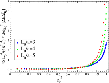
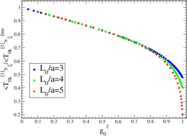
where stands for the expectation value of the action in Eq. (22). Although the quantities on the r.h.s. of Eq. (33) have values which are close to each other, their difference can be computed at a few permille accuracy with a moderate numerical effort. The difference has been computed for and at , and values of for and respectively. A sample of values is reported in Table 1, while all of them are shown in the left plot of Fig. 1. At each value of the points are interpolated with a cubic spline, and the resulting curve is integrated over . The free-case value is computed analytically by using Eq. (93), and is added to the integral. The systematics induced by the interpolation and the numerical integration of the data is negligible with respect to the statistical error.
To complete the calculation of , the expectation value is measured in a dedicated set of simulations. It is computed for and at , and values of for and respectively. A sample of values is reported in Table 2, and all of them are shown in the right plot of Fig. 1. By interpolating the results with a cubic spline, the renormalization constant is finally determined by the tree-level improved version of Eq. (29) given by
| (34) |
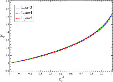
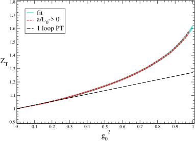
The results444Preliminary results have been reported in Ref. Giusti:2014tfa for at and and are shown in the left plot of Fig. 2. At the larger value of , discretization effects in are within our statistical errors. Those due to the finiteness of have been checked by computing555At this small volume we have computed either with the method described in this section, or with the Monte Carlo procedure in Ref. Giusti:2010bb . The numerical results are in agreement within statistical errors. at and in the full range of , and at and for . The results at for and are statistically compatible, and their central values differ at most by toward the larger values of . Since on the lattices with and those effects are expected to be suppressed at least by an additional factor of 1/8, we conclude that they are well within the statistical errors. We thus quote the values of at and as our best results in the limit , see right plot of Fig. 2. Even if defined by renormalization conditions which differ from ours by discretization effects, our values of at agree with those in Refs. Robaina:2013zmb ; Giusti:2014ila which, however, in many cases have a much larger statistical error.
IV.2 Determination of
The renormalization constant is computed by imposing the tree-level improved version of Eq. (31) given by
| (35) |
with
| (36) |
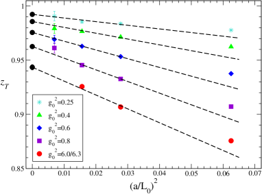
The latter condition guarantees that the WI remains valid at finite volume as it stands Giusti:2012yj . The expectation values of and of the difference are measured straightforwardly in the same Monte Carlo simulation666It is interesting to notice that the difference requires roughly 10 times the statistics needed for to meet the same relative statistical error.. The free case is subtracted analytically by using its expression in Appendix E. In practice we chose and so that the ratio of the spatial linear size over the temporal one is fixed to be . We simulated 5 values of in the range with temporal length and . The results for are given in Table 3, and they are shown in the left plot of Fig. 3. Discretization effects turn out to be quite larger than for at the smaller values of . Our best extrapolation to is given by the overall fit of the data at and to the function
| (37) |
The quality of the fit is very good, and it leads to the values of shown by the black points in the same plot. To check for the systematics associated to the extrapolation, we have performed a variety of different fits: we have removed the points at from our best fit, we have fit each set of points independently with a quadratic function in , we have amended the combined fit function by adding a quadratic term in to the coefficient of , and we have added a quadratic term in in Eq. (37). The results of all these fits are statistically compatible with those obtained in our best fit to the function in Eq. (37) and the selection of data points chosen. We take the maximum spread of the central values from the various fits as a systematic error due to the extrapolation, and we add it in quadrature to the statistical one. The final results are shown in the right plot of Fig. 3.
V Results and conclusions
The final results for are shown in the right plot of Fig. 2. They are very well represented by the expression
| (38) | |||||
in the full range , a function which coincide with the expansion in Eq. (III) to order . The deviation of the curve from the data is smaller than the statistical accuracy, see right plot of Fig. 2. The error to be attached to computed as in Eq. (38) is up to , while it grows linearly from to in the range . Within our statistical errors, the non-perturbative determination starts to deviate significantly from the one-loop result at .
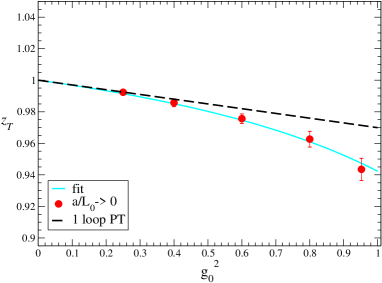
Our best results for are shown in the right plot of Fig. 3. In the full range , they are well represented by the expression
| (39) |
a function which again coincide with the expansion in
Eq. (III) to order . In this case the
error to be attached to the values in
Eq. (39) grows linearly from
to in the interval . The one loop
result agrees with the non-perturbative determination up to
within our statistical errors.
The above results for and clearly show that in the range of where the Wilson action is frequently simulated, one-loop perturbation theory is not adequate for computing the renormalization constants of the traceless components of the energy-momentum tensor defined as in Eq. (III). Shifted boundary conditions offer an extremely powerful tool to compute them, and therefore to define non-perturbatively the energy-momentum tensor on the lattice. The strategy implemented here can be easily generalized to QCD, and to (beyond Standard Model) QCD-like or supersymmetric theories.
Acknowledgements.
We thank H. B. Meyer and D. Robaina for interesting discussions in an early stage of this work. The simulations were performed on the BG/Q at CINECA (INFN and LISA agreement), on the PC cluster Zefiro of the INFN-CSN4 in Pisa, and on PC clusters at the Physics Department of the University of Milano-Bicocca. We thankfully acknowledge the computer resources and technical support provided by these institutions. This work was partially supported by the INFN SUMA project.Appendix A SU(3) conventions
The Lie algebra of SU(3) may be identified with the linear space of all hermitian traceless matrices. In the basis , , with
| (40) |
the elements of the algebra are linear combinations of them with real coefficients. The structure constants in the commutator relation
| (41) |
are real and totally anti-symmetric in the indices if the normalization condition
| (42) |
is imposed.
Appendix B Continuum notation
In the Euclidean space-time, the path integral of the SU(3) Yang–Mills theory is defined as
| (43) |
where the measures on gauge and ghost fields are defined as usual. The action is defined as
| (44) |
with
| (45) | |||||
where is the bare coupling constant, is the gauge-fixing parameter, the trace is over the color index and
| (46) | |||||
The ghost fields and are in the adjoint representation of the SU(3) group, i.e. and analogously for .
B.1 BRST transformations
The action (44) is invariant under the BRST transformations defined as Becchi:1974xu ; Becchi:1974md ; Tyutin:1975qk
| (47) | |||||
where is an infinitesimal Grassmann constant. They are nilpotent up to the equations of motion of the ghost field . In fact if we define
| (48) |
where is one of the fundamental fields which transforms as in Eqs. (B.1), it is easy to prove that777To this aim it is useful to notice that .
| (49) |
while
| (50) |
By using Eqs. (49) and (50) it is easy to show that the BRST transformations are nilpotent, up to the equation of motion of , when acting on any product of fundamental fields at arbitrary space-time points and thus on any functional of them.
The gauge-invariant part of the Yang–Mills action (44) is BRST-invariant because the BRST correspond to infinitesimal gauge transformations with parameter . The gauge-fixing part of the action turns out to be BRST-invariant too. It can also be written as a BRST rotation of a functional plus a term which, after integrating by parts, is proportional to the equation of motion of and serves to cancel the term coming from Eq. (50).
B.2 Equations of motion
The equations of motion for the gauge field are given by
| (51) |
where represents a generic string of fields, and the covariant derivative for the adjoint representation is defined as in Eq. (46), i.e.
| (52) |
The equations of motion for the ghosts are
| (53) | |||||
Appendix C Energy-momentum tensor in the continuum
The continuum theory is invariant under the group of space-time translations
| (54) |
where indicates generically one of the fields . The associated WIs can be derived in the usual way by studying the variation of the functional integral under local transformations parameterized by
| (55) |
The resulting integrated WIs are
| (56) |
where is the variation of the string of fields under the transformation (C). The canonical energy-momentum tensor of the theory can be written as
| (57) |
where
| (58) | |||||
For , Eq. (56) gives
| (60) |
and when all operators of the string are localized far away from , the classical conservation identities
| (61) |
are recovered. The canonical energy-momentum tensor is neither symmetric nor gauge invariant. To make it both symmetric and gauge invariant one applies the Belinfante procedure, and use the equation of motion. The resulting tensor satisfies the on-shell WIs in Eq. (61), and it gives the same conserved charges of the canonical tensor when inserted in on-shell correlation functions. The ambiguity left by the use of the equations of motion allows one to define the energy-momentum tensor as the one derived by exploiting the re-parameterization transformations of the theory coupled to an external gravitational field Callan:1970ze ; Adler:1976zt ; Collins:1976yq . All definitions related by terms which vanish by the equation of motion are equivalent provided the corresponding contact terms are taken into account in the WIs. The symmetric energy-momentum tensor is defined as
| (62) |
where
| (63) | |||||
By comparing Eqs. (57) and (62), it is quite easy to show that
| (64) |
i.e. the two four-divergences differ by terms which are proportional to the equations of motion. If we insert last equation in the WIs (60) and we use the the equations of motion (51) we arrive to
| (65) |
It is also useful to notice that
| (66) |
where is the BRST variation defined in appendix B and
When the interpolating operator is gauge-invariant, it is thus appropriate to define a gauge-invariant energy-momentum tensor
| (68) |
which satisfies
| (69) |
where the term proportional to the equation of motion of the ghosts is null because a gauge-invariant operator is independent of the field. The WIs (65) applies as well to without any modification. It is worth nothing that the gauge-invariant energy-momentum tensor generates the very same charges in on-shell correlation functions as all the other definitions in this appendix.
Appendix D Renormalization of the action density in dimensional regularization
In this appendix we report the essential formulas in dimensional regularization which are needed in the paper, for a recent review see Ref. Weisz:2010nr and reference therein. In dimensional regularization one replaces , and renormalizes the coupling constant as
| (70) |
where . The -function is
| (71) | |||||
where
| (72) |
and
| (73) |
with the number of colours being in our case.
In presence of shifted boundary conditions it holds
| (74) |
which can be written as ()
| (75) |
where and the renormalized density are defined in Eq. (16). The expectation values of the renormalized operators in Eq. (75) are finite and expandable in powers of . By following Ref. Luscher:2013lgggg , see also Ref. Suzuki:2013gza , the ratio
| (76) |
must then have a series in with no poles in . In dimensional regularization the coefficients of the poles in in the renormalization constants start at , and therefore
| (77) |
which implies
| (78) |
If we expand in the denominator we obtain
| (79) |
Since this quantity cannot have poles in
| (80) |
and therefore
| (81) |
The renormalization constant of the energy-density operator is unambiguously fixed from the one of the coupling.
Appendix E Lattice free theory with shifted boundary conditions
In this appendix we report the results for the expectation values of , (no sum over k), , and in the free theory on the lattice888The lattice spacing is set to in this appendix.. In the infinite volume limit the expectation value of the momentum density is given by Giusti:2012yj
| (82) |
where
| (83) |
If we notice that Giusti:2012yj
| (84) | |||||
where , and that real and imaginary parts of read
| (85) | |||||
| (86) |
we arrive to
| (87) |
Analogously, for the traceless diagonal component of the energy-momentum tensor we obtain
| (88) | |||
which by summing over gives
| (89) |
For the trace part we obtain
| (90) |
which by summing over gives
| (91) |
In the free theory the discrete derivative of the free energy in Eq. (30) is given by
| (92) |
which by summing over gives
| (93) |
All previous equations remain valid in finite volume if one makes the substitution
| (94) |
and defines a prescription for the zero mode.
Appendix F Numerical results
| 6.0 | 5.489(10) | 3.028(7) | 4.2564(33) |
|---|---|---|---|
| 6.03 | 4.886(10) | 2.443(6) | 3.8484(38) |
| 6.125 | 3.601(14) | 1.491(7) | 1.0016(28) |
| 6.5 | 1.576(11) | 5.160(37) | 2.339(20) |
| 7.0 | 7.65(8) | 2.232(33) | 8.88(11) |
| 8.0 | 2.96(5) | 7.08(25) | 2.43(9) |
| 9.0 | 1.604(38) | 3.60(17) | 1.09(11) |
| 10.0 | 1.041(23) | 2.07(8) | 6.6(9) |
| 11.0 | 7.77(22) | 1.49(8) | 3.8(6) |
| 12.0 | 5.85(25) | 1.06(6) | 3.2(5) |
| 13.5 | 4.29(35) | 7.9(8) | 2.0(6) |
| 17.0 | 2.39(14) | 3.8(5) | 1.3(4) |
| 20.0 | 1.52(12) | 2.8(4) | 8.2(28) |
| 24.0 | 1.14(8) | 2.16(27) | 4.6(24) |
| 30.0 | 7.5(6) | 1.48(26) | 5.5(14) |
| 50.0 | 2.99(23) | 6.6(8) | 2.3(7) |
| 80.0 | 1.25(15) | 2.09(39) | 0.97(37) |
For a representative sample of values of that we have simulated we collect the results for the difference of the average plaquettes entering Eq. (33) in Table 1, and the values of at in Table 2. The values of and for are given in Table 3.
| 6.0 | -5.2735(27) | -1.3772(13) | -2.826(9) |
|---|---|---|---|
| 6.03 | -5.3921(29) | -1.4447(11) | -4.047(6) |
| 6.125 | -5.6976(29) | -1.6064(13) | -5.568(5) |
| 6.3 | -6.1359(37) | -1.7977(12) | -6.797(6) |
| 6.5 | -6.5124(28) | -1.9495(12) | -7.610(7) |
| 7.0 | -7.1554(29) | -2.1899(20) | -8.786(7) |
| 8.0 | -7.9077(37) | -2.4488(20) | -9.916(8) |
| 9.0 | -8.3673(21) | -2.5947(30) | -10.550(7) |
| 10.0 | -8.6896(14) | -2.7002(32) | -10.981(8) |
| 11.0 | -8.9385(16) | -2.7780(31) | -11.288(6) |
| 12.0 | -9.1331(20) | -2.8358(20) | -11.538(6) |
| 13.5 | -9.3654(23) | -2.9111(16) | -11.822(6) |
| 17.0 | -9.7261(22) | -3.0181(16) | -12.276(6) |
| 20.0 | -9.9253(21) | -3.0862(17) | -12.525(6) |
| 24.0 | -10.1097(15) | -3.1420(17) | -12.768(7) |
| 30.0 | -10.2941(17) | -3.1987(18) | -12.995(6) |
| 40.0 | -10.4792(18) | -3.2587(6) | -13.240(6) |
| 60.0 | -10.6608(17) | -3.3148(7) | -13.446(7) |
| 6.3 | -4.1926(32) | -5.920(7) |
| 7.5 | -5.2711(17) | -7.228(5) |
| 10.0 | -6.1130(23) | -8.155(6) |
| 15.0 | -6.7612(22) | -8.825(6) |
| 24.0 | -7.2041(9) | -9.2798(23) |
| 6.3 | -0.7067(4) | -1.0642(14) |
| 7.5 | -0.9703(5) | -1.4242(14) |
| 10.0 | -1.1345(5) | -1.6321(13) |
| 15.0 | -1.2559(5) | -1.7761(14) |
| 24.0 | -1.3379(5) | -1.8703(14) |
| 6.3 | -0.18493(15) | -0.2839(6) |
| 7.5 | -0.29738(16) | -0.4475(5) |
| 10.0 | -0.35095(17) | -0.5190(5) |
| 15.0 | -0.38832(18) | -0.5666(5) |
| 24.0 | -0.41292(22) | -0.5972(6) |
| 7.5 | -0.05643(11) | -0.08597(37) |
| 10.0 | -0.06785(12) | -0.10255(35) |
| 15.0 | -0.07494(16) | -0.1121(5) |
| 24.0 | -0.08029(17) | -0.1188(5) |
References
- (1) S. Caracciolo, G. Curci, P. Menotti, and A. Pelissetto, The energy momentum tensor for lattice gauge theories, Annals Phys. 197 (1990) 119.
- (2) L. Giusti and H. B. Meyer, Thermal momentum distribution from path integrals with shifted boundary conditions, Phys.Rev.Lett. 106 (2011) 131601, [arXiv:1011.2727].
- (3) L. Giusti and H. B. Meyer, Thermodynamic potentials from shifted boundary conditions: the scalar-field theory case, JHEP 1111 (2011) 087, [arXiv:1110.3136].
- (4) L. Giusti and H. B. Meyer, Implications of Poincare symmetry for thermal field theories in finite-volume, JHEP 1301 (2013) 140, [arXiv:1211.6669].
- (5) M. Della Morte and L. Giusti, A novel approach for computing glueball masses and matrix elements in Yang-Mills theories on the lattice, JHEP 1105 (2011) 056, [arXiv:1012.2562].
- (6) H. Suzuki, Energy-momentum tensor from the Yang-Mills gradient flow, PTEP 2013 (2013), no. 8 083B03, [arXiv:1304.0533].
- (7) L. Del Debbio, A. Patella, and A. Rago, Space-time symmetries and the Yang-Mills gradient flow, JHEP 1311 (2013) 212, [arXiv:1306.1173].
- (8) H. Makino and H. Suzuki, Lattice energy-momentum tensor from the Yang-Mills gradient flow–inclusion of fermion fields, PTEP 2014 (2014), no. 6 063B02, [arXiv:1403.4772].
- (9) M. Lüscher, Small flow-time expansion of gauge-invariant local fields, Unpublished notes June 2013.
- (10) S. L. Adler, J. C. Collins, and A. Duncan, Energy-Momentum-Tensor Trace Anomaly in Spin 1/2 Quantum Electrodynamics, Phys.Rev. D15 (1977) 1712.
- (11) J. C. Collins, A. Duncan, and S. D. Joglekar, Trace and Dilatation Anomalies in Gauge Theories, Phys.Rev. D16 (1977) 438–449.
- (12) S. Caracciolo, P. Menotti, and A. Pelissetto, One loop analytic computation of the energy momentum tensor for lattice gauge theories, Nucl.Phys. B375 (1992) 195–242.
- (13) L. Giusti and M. Pepe, Equation of state of a relativistic theory from a moving frame, Phys.Rev.Lett. 113 (2014) 031601, [arXiv:1403.0360].
- (14) D. Robaina and H. B. Meyer, Renormalization of the momentum density on the lattice using shifted boundary conditions, PoS LATTICE2013 (2014) 323, [arXiv:1310.6075].
- (15) N. Cabibbo and E. Marinari, A New Method for Updating SU(N) Matrices in Computer Simulations of Gauge Theories, Phys. Lett. B119 (1982) 387–390.
- (16) P. de Forcrand, M. D’Elia, and M. Pepe, A study of the ’t Hooft loop in SU(2) Yang-Mills theory, Phys. Rev. Lett. 86 (2001) 1438, [hep-lat/0007034].
- (17) M. Della Morte and L. Giusti, Exploiting symmetries for exponential error reduction in path integral Monte Carlo, Comput. Phys. Commun. 180 (2009) 813–818.
- (18) L. Giusti and M. Pepe, Non-perturbative renormalization of the energy-momentum tensor in SU(3) Yang-Mills theory, Proc. Sci. LATTICE2014 (2015) 322
- (19) C. Becchi, A. Rouet, and R. Stora, The Abelian Higgs-Kibble Model. Unitarity of the S Operator, Phys.Lett. B52 (1974) 344.
- (20) C. Becchi, A. Rouet, and R. Stora, Renormalization of the Abelian Higgs-Kibble Model, Commun.Math.Phys. 42 (1975) 127–162.
- (21) I. Tyutin, Gauge Invariance in Field Theory and Statistical Physics in Operator Formalism, arXiv:0812.0580.
- (22) J. Callan, Curtis G., S. R. Coleman, and R. Jackiw, A New improved energy-momentum tensor, Annals Phys. 59 (1970) 42–73.
- (23) P. Weisz, Renormalization and lattice artifacts, arXiv:1004.3462.