Property-based Polynomial Invariant Generation using Sums-of-Squares Optimization

Abstract

While abstract interpretation is not theoretically restricted to specific kinds of properties, it is, in practice, mainly developed to compute linear over-approximations of reachable sets, aka. the collecting semantics of the program. The verification of user-provided properties is not easily compatible with the usual forward fixpoint computation using numerical abstract domains.

We propose here to rely on sums-of-squares programming to characterize a property-driven polynomial invariant. This invariant generation can be guided by either boundedness, or in contrary, a given zone of the state space to avoid.

While the target property is not necessarily inductive with respect to the program semantics, our method identifies a stronger inductive polynomial invariant using numerical optimization. Our method applies to a wide set of programs: a main while loop composed of a disjunction (if-then-else) of polynomial updates e.g. piecewise polynomial controllers. It has been evaluated on various programs.

1 Introduction

With the increased need for confidence in software, it becomes more than ever important to provide means to support the verification of specification of software. Among the various formal verification methods to support these analysis, a first line of approaches, such as deductive methods or SMT-based model checking, provide rich languages to support the expression of the specification and then try to discharge the associate proof obligation using automatic solvers. The current state of the art of these solvers is able to manipulate satisfiability problems over linear arithmetics or restricted fragments of non linear arithmetics. Another line of approaches, such as static analysis also known as abstract interpretation, restricts, a priori, the kind of properties considered during the computation: these methods typically perform interval arithmetic analysis or rely on convex polyhedra computations. In practice this second line of work seems more capable of manipulating and generating numerical invariants through the computation of inductive invariants, while the first line of approaches hardly synthesize these required invariants through satisfiability checks.

However, when it comes to more than linear properties, the state of the art is not well developed. In the early 2000s, ellipsoid analyses [Fer04], similar to restricted cases of Lyapunov functions, were designed to support the study of a family of Airbus controllers. This exciting result was used to provide the analysis of absence of runtime errors but could hardly be adapted to handle more general user provided specifications for polynomial programs.

However proving polynomial inequalities is NP-hard and boils down to show that the infimum of a given polynomial is nonnegative. Still, one can obtain lower bounds of such infima by decomposing certain nonnegative polynomials into sums-of-squares (SOS). This actually leads to solve hierarchies of semidefinite relaxations, introduced by Lasserre in [Las01]. Recent advances in semidefinite programming allowed to extensively apply these relaxations to various fields, including parametric polynomial optimization, optimal control, combinatorial optimization, etc. (see e.g. [Par03, Lau09] for more details).

While these approaches were mentioned a decade ago in [Cou05] and mainly applied to termination analysis, they hardly made their way through the software verification community to address more general properties.

Contributions.

Our contribution allows to analyze high level properties defined as a sublevel set of polynomials functions, i.e. basic semialgebraic sets. This class of properties is rather large: it ranges from boundedness properties to the definition of a bad region of the state space to avoid. While these properties, when they hold, are meant to be invariant, i.e. they hold in each reachable state, they are not necessarily inductive. Our approach rely on the computation of a stronger inductive property using SOS programming. This stronger property is proved inductive on the complete system and, by construction, implies the target property specified by the user. We develop our analysis on discrete-time piecewise polynomial systems, capturing a wide class of critical programs, as typically found in current embedded systems such as aircrafts.

Organization of the paper.

The paper is organized as follows. In Section 2, we present the programs that we want to analyze and their representation as piecewise polynomial discrete-time systems. Next, we recall in Section 3 the collecting semantics that we use and introduce the polynomial optimization problem providing inductive invariants based on target polynomial properties. Section 4 contains the main contribution of the paper, namely how to compute effectively such invariants with SOS programming. Practical computation examples are provided in Section 5. Finally, we explain in Section 6 how to derive template bases from generated invariants.

2 Polynomial programs and piecewise polynomial discrete-time systems

In this section, we describe the programs which are considered in this paper and we explain how to analyze them through their representation as piecewise polynomial discrete-time dynamical systems.

We focus on programs composed of a single loop with a possibly complicated switch-case type loop body. Moreover we suppose without loss of generality that the analyzed programs are written in Static Single Assignment (SSA) form, that is each variable is initialized at most once.

Definitions.

We recall that a function $f$ from $\mathbb{R}^{d}$ to $\mathbb{R}$ is a polynomial if and only if there exists $k\in\mathbb{N}$, a family $\{c_{\alpha}\mid\alpha=(\alpha_{1},\ldots,\alpha_{d})\in\mathbb{N}^{d},\ |\alpha|=\alpha_{1}+\ldots+\alpha_{d}\leq k\}$ such that for all $x\in\mathbb{R}^{d}$, $f(x)=\sum_{|\alpha|\leq k}c_{\alpha}x_{1}^{\alpha_{1}}\ldots x_{d}^{\alpha_{d}}$. By extension a function $f:\mathbb{R}^{d}\mapsto\mathbb{R}^{d}$ is a polynomial if and only if all its coordinate functions are polynomials. Let $\mathbb{R}[x]$ stands for the set of $d$-variate polynomials.

In this paper, we consider assignments of variables using only parallel polynomial assignments $(x_{1},\ldots,x_{d})=T(x_{1},\ldots,x_{d})$ where $(x_{1},\ldots,x_{d})$ is the vector of the program variables. Tests are either weak polynomial inequalities $r(x_{1},\ldots,x_{d})\leq 0$ or strict polynomial inequalities $r(x_{1},\ldots,x_{d})<0$. We assume that assignments are polynomials from $\mathbb{R}^{d}$ to $\mathbb{R}^{d}$ and test functions are polynomials from $\mathbb{R}^{d}$ to $\mathbb{R}$. In the program syntax, the notation $\ll$ will be either $\verb+<=+$ or $\verb+<+$. The form of the analyzed program is described in Figure 1.

⬇ x $\in$ $X^{\mathrm{in}}$; while ($r_{1}^{0}$(x)$\ll$0 and … and $r_{n_{0}}^{0}$(x)$\ll$0){ case ($r_{1}^{1}$(x)$\ll$0 and … and $r_{n_{1}}^{1}$(x)$\ll$0): x = $T^{1}$(x); case … case ($r_{i}^{1}$(x)$\ll$0 and … and $r_{n_{i}}^{1}$(x)$\ll$0): x = $T^{i}$(x); }

Figure 1: One-loop programs with nested conditional branches

A set $C\subseteq\mathbb{R}^{d}$ is said to be a basic semialgebraic set if there exist $g_{1},\ldots,g_{m}\in\mathbb{R}[x]$ such that $C=\{x\in\mathbb{R}^{d}\mid g_{j}(x)\ll 0,\forall\,j=1,\ldots,m\}$, where $\ll$ is used to encode either a strict or a weak inequality.

As depicted in Figure 1, an update $T^{i}:\mathbb{R}^{d}\to\mathbb{R}^{d}$ of the $i$-th condition branch is executed if and only if the conjunction of tests $r_{j}^{i}(x)\ll 0$ holds. In other words, the variable $x$ is updated by $T^{i}(x)$ if the current value of $x$ belongs to the basic semialgebraic set

$$X^{i}:=\{x\in\mathbb{R}^{d}\,|\,\forall j=1,\dots,n_{i},\ r_{j}^{i}(x)\ll 0\}\enspace.$$ (1)

Piecewise Polynomial Systems.

Consequently, we interpret programs as constrained piecewise polynomial discrete-time dynamical systems (PPS for short). The term piecewise means that there exists a partition $\{X^{i},i\in\mathcal{I}\}$ of $\mathbb{R}^{d}$ such that for all $i\in\mathcal{I}$, the dynamics of the system is represented by the following relation, for $k\in\mathbb{N}$:

$$\text{if }x_{k}\in X^{i}\cap X^{0},\ x_{k+1}=T^{i}(x_{k})\,.$$ (2)

We assume that $\mathcal{I}$ is finite and that the initial condition $x_{0}$ belongs to some compact basic semialgebraic set $X^{\mathrm{in}}$. For the program, $X^{\mathrm{in}}$ is the set where the variables are supposed to be initialized in. Since the test entry for the loop condition can be nontrivial, we add the term constrained and $X^{0}$ denotes the set representing the conjunctions of tests for the loop condition. The iterates of the PPS are constrained to live in $X^{0}$: if for some step $k\in\mathbb{N}$, $x_{k}\notin X^{0}$ then the PPS is stopped at this iterate with the terminal value $x_{k}$.

We define a partition as a family of nonempty sets such that:

$$\bigcup_{i\in\mathcal{I}}X^{i}=\mathbb{R}^{d},\ \forall\,i,j\in\mathcal{I},\ i\neq j,X^{i}\cap X^{j}\neq\emptyset\,.$$ (3)

From Equation (3), for all $k\in\mathbb{N}^{*}$ there exists a unique $i\in\mathcal{I}$ such that $x_{k}\in X^{i}$. A set $X^{i}$ can contain both strict and weak polynomial inequalities and characterizes the set of the $n_{i}$ conjunctions of tests polynomials $r_{j}^{i}$. Let $r^{i}=(r_{1}^{i},\ldots,r_{n_{i}}^{i})$ stands for the vector of tests functions associated to the set $X^{i}$. We suppose that the basic semialgebraic sets $X^{\mathrm{in}}$ and $X^{0}$ also admits the representation given by Equation (1) and we denote by $r^{0}$ the vector of tests polynomials $(r_{1}^{0},\ldots,r_{n_{0}}^{0})$ and by $r^{\mathrm{in}}$ the vector of test polynomials $(r_{1}^{\mathrm{in}},\ldots,r_{n_{\mathrm{in}}}^{\mathrm{in}})$. To sum up, we give a formal definition of PPS.

Definition 1 (PPS)

A constrained polynomial piecewise discrete-time dynamical system (PPS) is the quadruple $(X^{\mathrm{in}},X^{0},\mathcal{X},\mathcal{L})$ with:

• $X^{\mathrm{in}}\subseteq\mathbb{R}^{d}$ is the compact basic semialgebraic set of the possible initial conditions;

• $X^{0}\subseteq\mathbb{R}^{d}$ is the basic semialgebraic set where the state variable lives;

• $\mathcal{X}:=\{X^{i},i\in\mathcal{I}\}$ is a partition as defined in Equation (3);

• $\mathcal{L}:=\{T^{i},i\in\mathcal{I}\}$ is the family of the polynomials from $\mathbb{R}^{d}$ to $\mathbb{R}^{d}$, w.r.t. the partition $\mathcal{X}$ satisfying Equation (2).

From now on, we associate a PPS representation to each program of the form described at Figure 1. Since a program admits several PPS representations, we choose one of them, but this arbitrary choice does not change the results provided in this paper. In the sequel, we will often refer to the running example described in Example 1.

Example 1 (Running example)

The program below involves four variables and contains an infinite loop with a conditional branch in the loop body. The update of each branch is polynomial. The parameters $c_{ij}$ (resp. $d_{ij}$) are given parameters. During the analysis, we only keep the variables $x_{1}$ and $x_{2}$ since $oldx_{1}$ and $oldx_{2}$ are just memories.

⬇ $x_{1},x_{2}\in[a_{1},a_{2}]\times[b_{1},b_{2}]$; $oldx_{1}$ = $x_{1}$; $oldx_{2}$ = $x_{2}$; while (-1 <= 0){ $oldx_{1}$ = $x_{1}$; $oldx_{2}$ = $x_{2}$; case : $oldx_{1}$^2 + $oldx_{2}$^2 <= 1 : $x_{1}$ = $c_{11}$ * $oldx_{1}$^2 + $c_{11}$ * $oldx_{2}$^3; $x_{2}$ = $c_{21}$ * $oldx_{1}$^3 + $c_{22}$ * $oldx_{2}$^2; case : -$oldx_{1}$^2 - $oldx_{2}$^2 < -1 $x_{1}$ = $d_{11}$ * $oldx_{1}$^3 + $d_{12}$ * $oldx_{2}$^2; $x_{2}$ = $d_{21}$ * $oldx_{1}$^2 + $d_{22}$ * $oldx_{2}$^2; } }

The associated PPS corresponds to the quadruple $(X^{\mathrm{in}},X^{0},\{X^{1},X^{2}\},\{T^{1},T^{2}\})$, where the set of initial conditions is:

$$X^{\mathrm{in}}=[a_{1},a_{2}]\times[b_{1},b_{2}]\,,$$

the system is not globally constrained, i.e. the set $X^{0}$ in which the variable $x=(x_{1},x_{2})$ lies is:

$$X^{0}=\mathbb{R}^{d}\,,$$

the partition verifying Equation (3) is:

$$X^{1}=\{x\in\mathbb{R}^{2}\mid x_{1}^{2}+x_{2}^{2}\leq 1\},\quad X^{2}=\{x\in\mathbb{R}^{2}\mid-x_{1}^{2}-x_{2}^{2}<-1\}\,,$$

and the polynomials relative to the partition $\{X^{1},X^{2}\}$ are:

$$T^{1}(x)=\left(\begin{array}[]{c}c_{11}x_{1}^{2}+c_{12}x_{2}^{3}\\ c_{21}x_{1}^{3}+c_{22}x_{2}^{2}\end{array}\right)\text{ and }T^{2}(x)=\left(\begin{array}[]{c}d_{11}x_{1}^{3}+d_{12}x_{2}^{2}\\ d_{21}x_{1}^{2}+d_{22}x_{2}^{2}\end{array}\right)\enspace.$$

3 Program invariants as sublevel sets

The main goal of the paper is to decide automatically if a given property holds for the analyzed program, i.e. for all its reachable states. We are interested in numerical properties and more precisely in properties on the values taken by the $d$-uplet of the variables of the program. Hence, in our point-of-view, a property is just the membership of some set $P\subseteq\mathbb{R}^{d}$. In particular, we study properties which are valid after an arbitrary number of loop iterates. Such properties are called loop invariants of the program. Formally, we use the PPS representation of a given program and we say that $P$ is a loop invariant of this program if:

$$\forall\,k\in\mathbb{N},\ x_{k}\in P\,,$$

where $x_{k}$ is defined at Equation (2) as the state variable at step $k\in\mathbb{N}$ of the PPS representation of the program. Our approach addresses any property expressible as a polynomial level set property. This section defines formally these notions and develop our approach: synthesize a property-driven inductive invariant.

3.1 Collecting Semantics as postfixpoint characterization

Now, let us consider a program of the form described in Figure 1 and let us denote by $\mathcal{S}$ the PPS representation of this program. The set $\mathfrak{R}$ of reachable values is the set of all possible values taken by the state variable along the running of $\mathcal{S}$. We define $\mathfrak{R}$ as follows:

$$\mathfrak{R}=\bigcup_{k\in\mathbb{N}}T_{|_{X^{0}}}^{k}(X^{\mathrm{in}})$$ (4)

where $T_{|_{X^{0}}}$ is the restriction of $T$ on $X^{0}$ and $T_{|_{X^{0}}}$ is not defined outside $X^{0}$. To prove that a set $P$ is a loop invariant of the program is equivalent to prove that $\mathfrak{R}\subseteq P$. We can rewrite $\mathfrak{R}$ inductively:

$$\mathfrak{R}=X^{\mathrm{in}}\cup\bigcup_{i\in\mathcal{I}}T^{i}\left(\mathfrak{R}\cap X^{i}\cap X^{0}\right)\,.$$ (5)

Let us denote by $\wp(\mathbb{R}^{d})$ the set of subsets of $\mathbb{R}^{d}$ and introduce the map $F:\wp(\mathbb{R}^{d})\rightarrow\wp(\mathbb{R}^{d})$ defined by:

$$F(C)=X^{\mathrm{in}}\cup\bigcup_{i\in\mathcal{I}}T^{i}\left(C\cap X^{i}\cap X^{0}\right)$$ (6)

We equip $\wp(\mathbb{R}^{d})$ with the partial order of inclusion. The infimum is understood in this sense i.e. as the greatest lower bound with respect to this order. The smallest fixed point problem is:

$$\inf\left\{C\in\wp(\mathbb{R}^{d})\mid C=F(C)\right\}\,.$$

It is well-known from Tarski’s theorem that the solution of this problem exists, is unique and in this case, it corresponds to $\mathfrak{R}$. Tarski’s theorem also states that $\mathfrak{R}$ is the smallest solution of the following Problem:

$$\inf\left\{C\in\wp(\mathbb{R}^{d})\mid F(C)\subseteq C\right\}\,.$$

Note also that the map $F$ corresponds to a standard transfer function (or collecting semantics functional) applied to the PPS representation of a program. We refer the reader to [CC77] for a seminal presentation of this approach.

To prove that a subset $P$ is a loop invariant, it suffices to show that $P$ satisfies $F(P)\subseteq P$. In this case, such $P$ is called inductive invariant.

3.2 Considered properties: sublevel properties $\mathcal{P}_{\kappa,\alpha}$

In this paper, we consider special properties: those that are encoded with sublevel sets of a given polynomial function.

Definition 2 (Sublevel property)

Given a polynomial function $\kappa\in\mathbb{R}[x]$ and $\alpha\in\mathbb{R}\cup\{+\infty\}$, we define the sublevel property $\mathcal{P}_{\kappa,\alpha}$ as follows:

$$\mathcal{P}_{\kappa,\alpha}:=\{x\in\mathbb{R}^{d}\mid\kappa(x)\ll\alpha\}\,.$$

where $\ll$ denotes $\leq$ when $\alpha\in\mathbb{R}$ and denotes $<$ for $+\infty$. The expression $\kappa(x)<+\infty$ expresses the boundedness of $\kappa(x)$ without providing a specific bound $\alpha$.

Example 2 (Sublevel property examples)

Boundedness. When one wants to bound the reachable values of a system, we can try to bound the $l_{2}$-norm of the system: $\mathcal{P}_{\|\cdot\|_{2}^{2},\infty}$ with $\kappa(x)=\|x\|_{2}^{2}$. The use of $\alpha=\infty$ does not impose any bound on $\kappa(x)$.

Safe set. Similarly, it is possible to check whether a specific bound is matched. Either globally using the $l_{2}$-norm and a specific $\alpha$: $\mathcal{P}_{\|\cdot\|_{2}^{2},\alpha}$, or bounding the reachable values of each variable: $\mathcal{P}_{\kappa_{i},\alpha_{i}}$ with $\kappa_{i}:x\mapsto x_{i}$ and $\alpha_{i}\in\mathbb{R}$.

Avoiding bad regions. If the bad region can be encoded as a sublevel property $k(x)\leq 0$ then its negation $-k(x)\leq 0$ characterize the avoidance of that bad zone. Eg. if one wants to prove that the square norm of the program variables is always greater than 1, then we can consider the property $\mathcal{P}_{\kappa,\alpha}$ with $\kappa(x)=1-\|x\|_{2}^{2}$ and $\alpha=0$.

A sublevel property is called sublevel invariant when this property is a loop invariant. This turns out to be difficult to prove loop invariant properties while considering directly $\mathfrak{R}$, thus we propose to find a more tractable over-approximation of $\mathfrak{R}$ for which such properties hold.

3.3 Approach: compute a $\mathcal{P}_{\kappa,\alpha}$-driven inductive invariant $P$

In this subsection, we explain how to compute a $d$-variate polynomial $p\in\mathbb{R}[x]$ and a bound $w\in\mathbb{R}$, such that the polynomial sublevel sets $P:=\{x\in\mathbb{R}^{d}\mid p(x)\leq 0\}$ and $\mathcal{P}_{\kappa,w}$ satisfy:

$$\mathfrak{R}\subseteq P\subseteq\mathcal{P}_{\kappa,w}\subseteq\mathcal{P}_{\kappa,\alpha}\,.$$ (7)

The first (from the left) inclusion forces $P$ to be valid for the whole reachable values set. The second inclusion constraints all elements of $P$ to satisfy the given sublevel property for a certain bound $w$. The last inclusion requires that the bound $w$ is smaller than the desired level $\alpha$. When $\alpha=\infty$, any bound $w$ ensures the sublevel property.

Now, we derive sufficient conditions on $p$ and $w$ to satisfy Equation (7). We decompose the problem in two parts. To satisfy the first inclusion, i.e. ensure that $P$ is a loop invariant, it suffices to guarantee that $F(P)\subseteq P$, namely that $P$ is an inductive invariant. Using Equation (5), $P$ is an inductive invariant if and only if:

$$X^{\mathrm{in}}\cup\bigcup_{i\in\mathcal{I}}T^{i}\left(P\cap X^{i}\cap X^{0}\right)\subseteq P\,,$$

or equivalently:

$$\left\{\begin{array}[]{l}\displaystyle{X^{\mathrm{in}}\subseteq P}\,,\\ \displaystyle{\forall\,i\in\mathcal{I},\ T^{i}\left(P\cap X^{i}\cap X^{0}\right)\subseteq P\,.}\end{array}\right.$$ (8)

Thus, we obtain:

$$\left\{\begin{array}[]{lrl}&p(x)\leq 0\,,&\quad\forall x\in X^{\mathrm{in}}\,,\\ \forall\,i\in\mathcal{I}\,,&p\,(T^{i}(x))\leq 0\,,&\quad\forall x\in P\cap X^{i}\cap X^{0}\,.\end{array}\right.$$ (11)

Now, we are interested in the second and third inclusions at Equation (7) that is the sublevel property satisfaction. The condition $P\subseteq\mathcal{P}_{\kappa,w}\subseteq\mathcal{P}_{\kappa,\alpha}$ can be formulated as follows:

$$\kappa(x)\leq w\leq\alpha\,,\quad\forall x\in P\,.\\$$ (12)

We recall that we have supposed that $P$ is written as $\{x\in\mathbb{R}^{d}\mid p(x)\leq 0\}$ where $p\in\mathbb{R}[x]$. Finally, we provide sufficient conditions to satisfy both (11) and (12). Consider the following optimization problem:

$$\left\{\begin{array}[]{rll}\inf_{p\in\mathbb{R}[x],w\in\mathbb{R}}&\quad w\,,&\\ \text{s.t.}&\quad p(x)\leq 0\,,&\quad\forall x\in X^{\mathrm{in}}\,,\\ &\quad\forall\,i\in\mathcal{I}\,,p\,(T^{i}(x))\leq p(x)\,,&\quad\forall x\in X^{i}\cap X^{0}\,,\\ &\quad\kappa(x)\leq w+p(x)\,,&\quad\forall x\in\mathbb{R}^{d}\,.\end{array}\right.$$ (17)

We remark that $\alpha$ is not present in Problem (17). Indeed, since we minimize $w$, either there exists a feasible $w$ such that $w\leq\alpha$ and we can exploit this solution or such $w$ is not available and we cannot conclude. However, from Problem (17), we can extract $(p,w)$ and in the case where the optimal bound $w$ is greater than $\alpha$, we could use this solution with another method such as policy iteration [AGM15].

Lemma 1

Let $(p,w)$ be any feasible solution of Problem (17) with $w\leq\alpha$ or $w<\infty$ in the case of $\alpha=\infty$. Then $(p,w)$ satisfies both (11) and (12) with $P:=\{x\in\mathbb{R}^{d}\mid p(x)\leq 0\}$. Finally, $P$ and $\mathcal{P}_{\kappa,w}$ satisfy Equation (7).

In practice, we rely on sum-of-squares programming to solve a relaxed version of Problem (17).

4 Sums-of-Squares Programming for Invariant Generation

We first recall some basic background about sums-of-squares certificates for polynomial optimization. Let $\mathbb{R}[x]_{2m}$ stands for the set of polynomials of degree at most $2m$ and $\Sigma[x]\subset\mathbb{R}[x]$ be the cone of sums-of-squares (SOS) polynomials, that is $\Sigma[x]:=\{\,\sum_{i}q_{i}^{2},\,\text{ with }q_{i}\in\mathbb{R}[x]\,\}$. Our work will use the simple fact that for all $p\in\Sigma[x]$, then $p(x)\geq 0$ for all $x\in\mathbb{R}^{d}$ i.e. $\Sigma[x]$ is a restriction of the set of the nonnegative polynomials. For $q\in\mathbb{R}[x]_{2m}$, finding a SOS decomposition $q=\sum_{i}q_{i}^{2}$ valid over $\mathbb{R}^{d}$ is equivalent to solve the following matrix linear feasibility problem:

$$q(x)=b_{m}(x)^{T}\,Q\,b_{m}(x)\,,\quad\forall x\in\mathbb{R}^{d},\,$$ (18)

where $b_{m}(x):=(1,x_{1},\dots,x_{d},x_{1}^{2},x_{1}x_{2},\dots,x_{d}^{m})$ (the vector of all monomials in $x$ up to degree $m$) and $Q$ being a semidefinite positive matrix (i.e. all the eigenvalues of $Q$ are nonnegative). The size of $Q$ (as well as the length of $b_{m}$) is ${d+m\choose d}$.

Example 3

consider the bi-variate polynomial $q(x):=1+x_{1}^{2}-2x_{1}x_{2}+x_{2}^{2}$. With $b_{1}(x)=(1,x_{1},x_{2})$, one looks for a semidefinite positive matrix $Q$ such that the polynomial equality $q(x)=b_{1}(x)^{T}\,Q\,b_{1}(x)$ holds for all $x\in\mathbb{R}^{2}$. The matrix

$$Q=\begin{pmatrix}1&0&0\\ 0&1&-1\\ 0&-1&1\end{pmatrix}$$

satisfies this equality and has three nonnegative eigenvalues, which are 0, 1, and 2, respectively associated to the three eigenvectors $e_{0}:=(0,1,1)^{\intercal}$, $e_{1}:=(1,0,0)^{\intercal}$ and $e_{2}:=(0,1,-1)^{\intercal}$. Defining the matrices $L:=(e_{1}\,e_{2}\,e_{0})=\begin{pmatrix}1&0&0\\ 0&1&1\\ 0&-1&1\end{pmatrix}$ and $D=\begin{pmatrix}1&0&0\\ 0&2&0\\ 0&0&0\end{pmatrix}$, one obtains the decomposition $Q=L^{\intercal}\,D\,L$ and the equality $q(x)=(L\,b_{1}(x))^{T}\,D\,(L\,b_{1}(x))=\sigma(x)=1+(x_{1}-x_{2})^{2}$, for all $x\in\mathbb{R}^{2}$. The polynomial $\sigma$ is called a SOS certificate and guarantees that $q$ is nonnegative.

In practice, one can solve the general problem (18) by using semidefinite programming (SDP) solvers (e.g. Mosek [AA00], SDPA [YFN⁺10]). For more details about SDP, we refer the interested reader to [VB94].

One way to strengthen the three nonnegativity constraints of Problem (17) is to consider the following hierarchy of SOS programs, parametrized by the integer $m$ representing the half of the degree of $p$:

$$\left\{\begin{aligned} \inf_{p\in\mathbb{R}[x]_{2m},w\in\mathbb{R}}&\quad w\enspace,\\ \text{s.t.}&\quad-p=\sigma_{0}-\sum_{j=1}^{n_{\mathrm{in}}}\sigma_{j}r_{j}^{\mathrm{in}}\enspace,\\ &\quad\forall\,i\in\mathcal{I},\ \displaystyle{p-p\circ T^{i}=\sigma^{i}-\sum_{j=1}^{n_{i}}\mu_{j}^{i}r_{j}^{i}-\sum_{j=1}^{n_{0}}\gamma_{j}^{i}r_{j}^{0}}\enspace,\\ &\quad\displaystyle{w+p-\kappa=\psi}\enspace,\\ &\\ &\quad\forall\,j=1,\ldots,n_{\mathrm{in}}\enspace,\ \sigma_{j}\in\Sigma[x]\enspace,\ \deg(\sigma_{j}r_{j}^{\mathrm{in}})\leq 2m\enspace,\\ &\quad\sigma_{0}\in\Sigma[x]\enspace,\ \deg(\sigma_{0})\leq 2m\enspace,\\ &\quad\forall\,i\in\mathcal{I}\enspace,\ \sigma^{i}\in\Sigma[x]\enspace,\ \deg(\sigma^{i})\leq 2m\deg T^{i}\enspace,\\ &\quad\forall\,i\in\mathcal{I}\enspace,\ \forall\,j=1,\ldots,n_{i}\enspace,\ \mu_{j}^{i}\in\Sigma[x]\enspace,\ \deg(\mu_{j}^{i}r_{j}^{i})\leq 2m\deg T^{i}\enspace,\\ &\quad\forall\,i\in\mathcal{I}\enspace,\ \forall\,j=1,\ldots,n_{0}\enspace,\ \gamma^{i}\in\Sigma[x]\enspace,\ \deg(\gamma_{j}^{i}r_{j}^{0})\leq 2m\deg T^{i}\enspace,\\ &\quad\psi\in\Sigma[x]\enspace,\ \deg(\psi)\leq 2m\enspace.\\ \end{aligned}\right.$$ (19)

Proposition 1

For a given $m\in\mathbb{N}$, let $(p_{m},w_{m})$ be any feasible solution of Problem (19). Then $(p_{m},w_{m})$ is also a feasible solution of Problem (17). Moreover, if $w_{m}\leq\alpha$ then both $P_{m}:=\{x\in\mathbb{R}^{d}\mid p_{m}(x)\leq 0\}$ and $\mathcal{P}_{\kappa,w_{m}}$ satisfy Equation (7).

Proof

The feasible solution $(p_{m},w_{m})$ is associated with SOS certificates ensuring that the three equality constraints of Problem (19) hold: $\{\sigma_{0},\sigma_{j}\}$ is associated to the first one, $\{\sigma^{i},\mu_{j}^{i},\gamma_{j}^{i}\}$ is associated to the second one and $\psi$ is associated to the third one. The first equality constraint, namely

$$-p_{m}(x)=\sigma_{0}(x)-\sum_{j=1}^{n_{\mathrm{in}}}\sigma_{j}(x)r_{j}^{\mathrm{in}}(x)\,,\quad\forall x\in\mathbb{R}^{d}\,,$$

implies that $\forall x\in X^{\mathrm{in}}\,,p_{m}(x)\leq 0$. Similarly, one has $\forall i\in\mathcal{I},\forall x\in X^{i}\cap X^{0},p_{m}\,(T^{i}(x))\leq p_{m}(x)$ and $\forall x\in\mathbb{R}^{d},\kappa(x)\leq w_{m}+p_{m}(x)$. Then $(p_{m},w_{m})$ is a feasible solution of Problem (17). The second statement comes directly from Lemma 1.

Computational considerations.

Define $t:=\max\{\deg T^{i},i\in\mathcal{I}\}$. At step $m$ of this hierarchy, the number of SDP variables is proportional to $\binom{d+2mt}{d}$ and the number of SDP constraints is proportional to $\binom{d+mt}{d}$. Thus, one expects tractable approximations when the number $d$ of variables (resp. the degree $2m$ of the template $p$) is small. However, one can handle bigger instances of Problem (19) by taking into account the system properties. For instance one could exploit sparsity as in [WKKM06] by considering the variable sparsity correlation pattern of the polynomials $\{T^{i},i\in\mathcal{I}\},\{r_{j}^{i},i\in\mathcal{I},j=1,\ldots,n_{i}\},\{r_{j}^{0},j=1,\ldots,n_{0}\},\{r_{j}^{\mathrm{in}},j=1,\ldots,n_{\mathrm{in}}\}$ and $\kappa$.

5 Benchmarks

Here, we perform some numerical experiments while solving Problem (19) (given in Section 4) on several examples. In Section 5.1, we verify that the program of Example 1 satisfies some boundedness property. We also provide examples involving higher dimensional cases. Then, Section 5.2 focuses on other properties, such as checking that the set of variable values avoids an unsafe region. Numerical experiments are performed on an Intel Core i5 CPU ($2.40\,$GHz) with Yalmip being interfaced with the SDP solver Mosek.

5.1 Checking boundedness of the set of variables values

Example 4

Following Example 1, we consider the constrained piecewise discrete-time dynamical system $\mathcal{S}=(X^{\mathrm{in}},X^{0},\{X^{1},X^{2}\},\{T^{1},T^{2}\})$ with $X^{\mathrm{in}}=[0.9,1.1]\times[0,0.2]$, $X^{0}=\{x\in\mathbb{R}^{2}\mid r^{0}(x)\leq 0\}$ with $r^{0}:x\mapsto-1$, $X^{1}=\{x\in\mathbb{R}^{2}\mid r^{1}(x)\leq 0\}$ with $r^{1}:x\mapsto\mbox{$\|x\|$}^{2}-1$, $X^{2}=\{x\in\mathbb{R}^{2}\mid r^{2}(x)<0\}$ with $r^{2}=-r^{1}$ and $T^{1}:(x_{1},x_{2})\mapsto(c_{11}x_{1}^{2}+c_{12}x_{2}^{3},c_{21}x_{1}^{3}+c_{22}x_{2}^{2})$, $T^{2}:(x_{1},x_{2})\mapsto(d_{11}x_{1}^{3}+d_{12}x_{2}^{2},d_{21}x_{1}^{2}+d_{22}x_{2}^{2})$. We are interested in showing that the boundedness property $\mathcal{P}_{\|\cdot\|_{2}^{2},\alpha}$ holds for some positive $\alpha$.

(a) $m=3$

(b) $m=4$

(c) $m=5$

Figure 2: A hierarchy of sublevel sets $P_{m}$ for Example 4

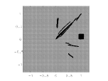
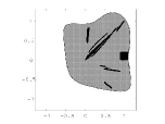
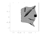
Here we illustrate the method by instantiating the program of Example 1 with the following input: $a_{1}=0.9$, $a_{2}=1.1$, $b_{1}=0$, $b_{2}=0.2$, $c_{11}=c_{12}=c_{21}=c_{22}=1$, $d_{11}=0.5$, $d_{12}=0.4$, $d_{21}=-0.6$ and $d_{22}=0.3$. We represent the possible initial values taken by the program variables $(x_{1},x_{2})$ by picking uniformly $N$ points $(x_{1}^{(i)},x_{2}^{(i)})\ (i=1,\dots,N)$ inside the box $X^{\mathrm{in}}=[0.9,1.1]\times[0,0.2]$ (see the corresponding square of dots on Figure 2). The other dots are obtained after successive updates of each point $(x_{1}^{(i)},x_{2}^{(i)})$ by the program of Example 1. The sets of dots in Figure 2 are obtained with $N=100$ and six successive iterations.

At step $m=3$, Program (19) yields a solution $(p_{3},w_{3})\in\mathbb{R}_{6}[x]\times\mathbb{R}$ together with SOS certificates, which guarantee the boundedness property, that is $x\in\mathfrak{R}\implies x\in P_{3}:=\{p_{3}(x)\leq 0\}\subseteq\mathcal{P}_{\|\cdot\|_{2}^{2},w_{3}}\implies\|x\|_{2}^{2}\leq w_{3}$. One has $p_{3}(x):=-2.510902467-0.0050x_{1}-0.0148x_{2}+3.0998x_{1}^{2}-0.8037x_{2}^{3}-3.0297x_{1}^{3}+2.5924x_{2}^{2}+1.5266x_{1}x_{2}-1.9133x_{1}^{2}x_{2}-1.8122x_{1}x_{2}^{2}+1.6042x_{1}^{4}+0.0512x_{1}^{3}x_{2}-4.4430x_{1}^{2}x_{2}^{2}-1.8926x_{1}x_{2}^{3}+0.5464x_{2}^{4}-0.2084x_{1}^{5}+0.5866x_{1}^{4}x_{2}+2.2410x_{1}^{3}x_{2}^{2}+1.5714x_{1}^{2}x_{2}^{3}-0.0890x_{1}x_{2}^{4}-0.9656x_{2}^{5}+0.0098x_{1}^{6}-0.0320x_{1}^{5}x_{2}-0.0232x_{1}^{4}x_{2}^{2}+0.2660x_{1}^{3}x_{2}^{3}+0.7746x_{1}^{2}x_{2}^{4}+0.9200x_{1}x_{2}^{5}+0.6411x_{2}^{6}$ (for the sake of conciseness, we do not display $p_{4}$ and $p_{5}$).

Figure 2 displays in light gray outer approximations of the set of possible values $X_{1}$ taken by the program of Example 4 as follows: (a) the degree six sublevel set $P_{3}$, (b) the degree eight sublevel set $P_{4}$ and (c) the degree ten sublevel set $P_{5}$. The outer approximation $P_{3}$ is coarse as it contains the box $[-1.5,1.5]^{2}$. However, solving Problem (19) at higher steps yields tighter outer approximations of $\mathfrak{R}$ together with more precise bounds $w_{4}$ and $w_{5}$ (see the corresponding row in Table 2).

We also succeeded to certify that the same property holds for higher dimensional programs, described in Example 5 ($d=3$) and Example 6 ($d=4$).

Example 5

Here we consider $X^{\mathrm{in}}=[0.9,1.1]\times[0,0.2]^{2}$, $r^{0}:x\mapsto-1$, $r^{1}:x\mapsto\|x\|_{2}^{2}-1$, $r^{2}=-r^{1}$, $T^{1}:(x_{1},x_{2},x_{3})\mapsto 1/4(0.8x_{1}^{2}+1.4x_{2}-0.5x_{3}^{2},1.3x_{1}+0.5x_{3}^{2},1.4x_{2}+0.8x_{3}^{2})$, $T^{2}:(x_{1},x_{2},x_{3})\mapsto 1/4(0.5x_{1}+0.4x_{2}^{2},-0.6x_{2}^{2}+0.3x_{3}^{2},0.5x_{3}+0.4x_{1}^{2})$ and $\kappa:x\mapsto\|x\|_{2}^{2}$.

Example 6

Here we consider $X^{\mathrm{in}}=[0.9,1.1]\times[0,0.2]^{3}$, $r^{0}:x\mapsto-1$, $r^{1}:x\mapsto\|x\|_{2}^{2}-1$, $r^{2}=-r^{1}$, $T^{1}:(x_{1},x_{2},x_{3},x_{4})\mapsto 0.25(0.8x_{1}^{2}+1.4x_{2}-0.5x_{3}^{2},1.3x_{1}+0.5,x_{2}^{2}-0.8x_{4}^{2},0.8x_{3}^{2}+1.4x_{4},1.3x_{3}+0.5x_{4}^{2})$, $T^{2}:(x_{1},x_{2},x_{3},x_{4})\mapsto 0.25(0.5x_{1}+0.4x_{2}^{2},-0.6x_{1}^{2}+0.3x_{2}^{2},0.5x_{3}+0.4x_{4}^{2},-0.6x_{3}+0.3x_{4}^{2})$ and $\kappa:x\mapsto\|x\|_{2}^{2}$.

Table 1 reports several data obtained while solving Problem (19) at step $m$, ($2\leq m\leq 5$), either for Example 4, Example 5 or Example 6. Each instance of Problem (19) is recast as a SDP program, involving a total number of “Nb. vars” SDP variables, with a SDP matrix of size “Mat. size”. We indicate the CPU time required to compute the optimal solution of each SDP program with Mosek.

The symbol “$-$” means that the corresponding SOS program could not be solved within one day of computation. These benchmarks illustrate the computational considerations mentioned in Section 4 as it takes more CPU time to analyze higher dimensional programs. Note that it is not possible to solve Problem (19) at step $5$ for Example 6. A possible workaround to limit this computational blow-up would be to exploit the sparsity of the system.

Table 1: Comparison of timing results for Example 4, 5 and 6

Degree $2m$		4	6	8	10
Example 4	Nb. vars	1513	5740	15705	35212
	Mat. size	368	802	1404	2174
($d=2$)	Time	$0.82\,s$	$1.35\,s$	$4.00\,s$	$9.86\,s$
Example 5	Nb. vars	2115	11950	46461	141612
	Mat. size	628	1860	4132	7764
($d=3$)	Time	$0.84\,s$	$2.98\,s$	$21.4\,s$	$109\,s$
Example 6	Nb. vars	7202	65306	18480	$-$
	Mat. size	1670	6622	373057	$-$
($d=4$)	Time	$2.85\,s$	$57.3\,s$	$1534\,s$	$-$

Table 2: Hierarchies of bounds obtained for various properties

Benchmark	$\kappa$	$w_{2}$	$w_{3}$	$w_{4}$	$w_{5}$
Example 4	$\|\cdot\|_{2}^{2}$	639	17.4	2.44	2.02
Example 7	$x\mapsto 0.25-\|x+0.5\|_{2}^{2}$	0.25	0.249	0.0993	-0.0777
Example 8	$\|\cdot\|_{2}^{2}$	10.2	2.84	2.84	2.84
	$x\mapsto\|T^{1}(x)-T^{2}(x)\|_{2}^{2}$	5.66	2.81	2.78	2.78

5.2 Other properties

Here we consider the program given in Example 7. One is interested in showing that the set $X_{1}$ of possible values taken by the variables of this program does not meet the ball $B$ of center $(-0.5,-0.5)$ and radius $0.5$.

Example 7

Let consider the PPS $\mathcal{S}=(X^{\mathrm{in}},X^{0},\{X^{1},X^{2}\},\{T^{1},T^{2}\})$ with $X^{\mathrm{in}}=[0.5,0.7]\times[0.5,0.7]$, $X^{0}=\{x\in\mathbb{R}^{2}\mid r^{0}(x)\leq 0\}$ with $r^{0}:x\mapsto-1$, $X^{1}=\{x\in\mathbb{R}^{2}\mid r^{1}(x)\leq 0\}$ with $r^{1}:x\mapsto\|x\|_{2}^{2}-1$, $X^{2}=\{x\in\mathbb{R}^{2}\mid r^{2}(x)\leq 0\}$ with $r^{2}=-r^{1}$ and $T^{1}:(x_{1},x_{2})\mapsto(x_{1}^{2}+x_{2}^{3},x_{1}^{3}+x_{2}^{2})$, $T^{2}:(x,y)\mapsto(0.5x_{1}^{3}+0.4x_{2}^{2},-0.6x_{1}^{2}+0.3x_{2}^{2})$. With $\kappa:(x_{1},x_{2})\mapsto 0.25-(x_{1}+0.5)^{2}-(x_{2}+0.5)^{2}$, one has $B:=\{x\in\mathbb{R}^{2}\mid 0\leq\kappa(x)\}$. Here, one shall prove $x\in\mathfrak{R}\implies\kappa(x)<0$ while computing some negative $\alpha$ such that $\mathfrak{R}\subseteq\mathcal{P}_{\kappa,\alpha}$. Note that $\kappa$ is not a norm, by contrast with the previous examples.

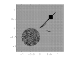
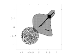
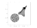
At step $m=3$ (resp.$m=4$), Program (19) yields a nonnegative solution $w_{3}$ (resp. $w_{4}$). Hence, it does not allow to certify that $\mathfrak{R}\cap B$ is empty. This is illustrated in both Figure 3 (a) and Figure 3 (b), where the light grey region does not avoid the ball $B$. However, solving Program (19) at step $m=5$ yields a negative bound $w_{5}$ together with a certificate that $\mathfrak{R}$ avoids the ball $B$ (see Figure 3 (c)). The corresponding values of $w_{m}$ ($m=3,4,5$) are given in Table 2.

(a) $m=3$

(b) $m=4$

(c) $m=5$

Figure 3: A hierarchy of sublevel sets $P_{m}$ for Example 7

Finally, one analyzes the program given in Example 8.

Example 8

(adapted from Example 3 in [AJ13])

Let $\mathcal{S}$ be the PPS $(X^{\mathrm{in}},X^{0},\{X^{1},X^{2}\},\{T^{1},T^{2}\})$ with $X^{\mathrm{in}}=[-1,1]\times[-1,1]$, $X^{0}=\{x\in\mathbb{R}^{2}\mid r^{0}(x)\leq 0\}$ with $r^{0}:x\mapsto-1$, $X^{1}=\{x\in\mathbb{R}^{2}\mid r^{1}(x)\leq 0\}$ with $r^{1}:x\mapsto x_{2}-x_{1}$, $X^{2}=\{x\in\mathbb{R}^{2}\mid r^{2}(x)\leq 0\}$ with $r^{2}=-r^{1}$ and $T^{1}:(x_{1},x_{2})\mapsto(0.687x_{1}+0.558x_{2}-0.0001*x_{1}x_{2},-0.292x_{1}+0.773x_{2})$, $T^{2}:(x,y)\mapsto(0.369x_{1}+0.532x_{2}-0.0001x_{1}^{2},-1.27x_{1}+0.12x_{2}-0.0001x_{1}x_{2})$. We consider the boundedness property $\kappa_{1}:=\|\cdot\|_{2}^{2}$ as well as $\kappa_{2}(x):=\|T^{1}(x)-T^{2}(x)\|_{2}^{2}$. The function $\kappa_{2}$ can be viewed as the absolute error made by updating the variable $x$ after a possibly “wrong” branching. Such behaviors could occur while computing wrong values for the conditionals (e.g. $r^{1}$) using floating-point arithmetics. Table 2 indicates the hierarchy of bounds obtained after solving Problem (19) with $m=3,4,5$, for both properties. The bound $w_{5}=2.84$ (for $\kappa_{1}$) implies that the set of reachable values may not be included in the initial set $X^{\mathrm{in}}$. A valid upper bound of the error function $\kappa_{2}$ is given by $w_{5}=2.78$.

6 Templates bases

We finally present further use of the set $P$ defined at Equation (7). This sublevel set can be viewed as a template abstraction, following from the definition in [AGG11], with a fixed template basis ${p}$ and an associated $0$ bound. This representation allows to develop a policy iteration algorithm [AGM15] to obtain more precise inductive invariants.

We now give some simple method to complete this template basis to improve the precision of the bound $w$ found with Problem (19).

Proposition 2 (Template basis completions)

Let $(p,w)$ be a solution of Problem (19) and $\mathcal{Q}$ be a finite subset of $\mathbb{R}[x]$ such that for all $q\in\mathcal{Q}$, $p-q\in\Sigma[x]$. Then $\mathfrak{R}\subseteq\{x\in\mathbb{R}^{d}\mid p(x)\leq 0,\ q(x)\leq 0,\ \forall\,q\in\mathcal{Q}\}\subseteq\mathcal{P}_{\kappa,w}\subseteq\mathcal{P}_{\kappa,\alpha}$ and $\{x\in\mathbb{R}^{d}\mid p(x)\leq 0,\ q(x)\leq 0,\ \forall\,q\in\mathcal{Q}\}$ is an inductive invariant.

Proof

Let $Q$ be the set $\{x\in\mathbb{R}^{d}\mid p(x)\leq 0,\ q(x)\leq 0,\ \forall\,q\in\mathcal{Q}\}$. It is obvious that $Q\subseteq P=\{x\in\mathbb{R}^{d}\mid p(x)\leq 0\}$ and hence $Q\subseteq\mathcal{P}_{\kappa,w}$. Now let us prove that $Q$ is an inductive invariant. We have to prove that $Q$ satisfies Equation (8) that is: (i) For all $x\in X^{\mathrm{in}}$, $q(x)\leq 0$; (ii) For all $i\in\mathcal{I}$, for all $x\in Q\cap X^{i}\cap X^{0}$, $q(T^{i}(x))\leq 0$. For all $q\in\mathcal{Q}$, we denote by $\psi_{q}$ the element of $\Sigma[x]$ such that $p-q=\psi_{q}$. Let us show (i) and let $x\in X^{\mathrm{in}}$. We have $q(x)=p(x)-\psi_{q}(x)$ and since $\psi_{q}\in\Sigma[x]$, we obtain, $q(x)\leq p(x)$. Now from Proposition 1 and Lemma 1 and since $(p,w)$ is a solution of Problem (19), we conclude that $q(x)\leq p(x)\leq 0$.

Now let us prove (ii) and let $i\in\mathcal{I}$ and $x\in Q\cap X^{i}\cap X^{0}$. We get $q(T^{i}(x))=p(T^{i}(x))-\psi_{q}(T^{i}(x))$ and since $\psi_{q}\in\Sigma[x]$, we obtain $q(T^{i}(x))\leq p(T^{i}(x))$. Using the fact that $(p,w)$ is a solution of Problem (19) and using Proposition 1 and Lemma 1, we obtain $q(T^{i}(x))\leq p(T^{i}(x))\leq p(x)$. Since $x\in Q\subseteq P=\{y\in\mathbb{R}^{d}\mid p(y)\leq 0\}$, we conclude that $q(T^{i}(x))\leq 0$.

Actually, we can weaken the hypothesis of Proposition 2 to construct an inductive invariant. Indeed, after the computation of $p$ following Problem (19), it suffices to take a polynomial $q$ such that $p-q\geq 0$. Nevertheless, we cannot compute easily such a polynomial $q$. By using the hypothesis $p-q\in\Sigma[x]$, we can compute $q$ by sum-of-squares. Proposition 2 allows to define a simple method to construct a basic semialgebraic inductive invariant set. Then the polynomials describing this basic semialgebraic set defines a new templates basis and this basic semialgebraic set can be used as initialisation of the policy iteration algorithm developed in [AGM15]. Note that the link between the templates generation and the initialisation of policy iteration has been addressed in [Adj14].

Example 9

Let us consider the property $\mathcal{P}_{\|\cdot\|_{2}^{2},\infty}$ and let $(p,w)$ be a solution of Problem (19). We have $\kappa(x)=\sum_{1\leq j\leq k}x_{j}^{2}$ and $w+p-\kappa=\psi$ where $\psi\in\Sigma[x]$. In [RJGF12], the templates basis used to compute bounds on the reachable values set consists in the square variables plus a Lyapunov function. Let us prove that, in our setting, $\mathcal{Q}=\{x_{k}^{2}-w,\ k=1,\ldots,d\}$ can complete $\{p\}$ in the sense of Proposition 2. Let $k\in\{1,\ldots,d\}$ and let $x\in\mathbb{R}^{d}$, $p(x)-(x_{k}^{2}-w)=p(x)-\kappa(x)+w+\sum_{j\neq k}x_{j}^{2}=\psi(x)+\sum_{j\neq k}x_{j}^{2}\in\Sigma[x]$.

7 Related works and conclusion

Roux et al. [RJGF12] provide an automatic method to compute floating-point certified Lyapunov functions of perturbed affine loop body updates. They use Lyapunov functions with squares of coordinate functions as quadratic invariants in case of single loop programs written in affine arithmetic. In the context of hybrid systems, certified inductive invariants can be computed by using SOS approximations of parametric polynomial optimization problems [LWYZ14]. In [PJ04], the authors develop a SOS-based methodology to certify that the trajectories of hybrid systems avoid an unsafe region.

In the context of static analysis for semialgebraic programs, the approach developed in [Cou05] focuses on inferring valid loop/conditional invariants for semialgebraic programs. This approach relaxes an invariant generation problem into the resolution of nonlinear matrix inequalities, handled with semidefinite programming. Our method bears similarities with this approach but we generate a hierarchy of invariants (of increasing degree) with respect to target polynomial properties and restrict ourselves to linear matrix inequality formulations. In [BRCZ05], invariants are given by polynomial inequalities (of bounded degree) but the method relies on a reduction to linear inequalities (the polyhedra domain). Template polyhedra domains allow to analyze reachability for polynomial systems: in [STDG12], the authors propose a method that computes linear templates to improve the accuracy of reachable set approximations, whereas the procedure in [DT12] relies on Bernstein polynomials and linear programming, with linear templates being fixed in advance. Bernstein polynomials also appear in  [RG13] as polynomial templates but they are not generated automatically. In [SG09], the authors use SMT-based techniques to automatically generate templates which are defined as formulas built with arbitrary logical structures and predicate conjunctions. Other reductions to systems of polynomial equalities (by contrast with polynomial inequalities, as we consider here) were studied in [MOS04, RCK07] and more recently in [CJJK14].

In this paper, we give a formal framework to relate the invariant generation problem to the property to prove on analyzed program. We proposed a practical method to compute such invariants in the case of polynomial arithmetic using sums-of-squares programming. This method is able to handle non trivial examples, as illustrated through the numerical experiments. Topics of further investigation include refining the invariant bounds generated for a specific sublevel property, by applying the policy iteration algorithm. Such a refinement would be of particular interest if one can not decide whether the set of variable values avoids an unsafe region when the bound of the corresponding sums-of-squares program is not accurate enough. For the case of boundedness property, it would allow to decrease the value of the bounds on the variables. Finally, our method could be generalized to a larger class of programs, involving semialgebraic or transcendental assignments, while applying the same polynomial reduction techniques as in [MAGW14].

References

- [AA00] Erling D. Andersen and Knud D. Andersen. The mosek interior point optimizer for linear programming: An implementation of the homogeneous algorithm. In Hans Frenk, Kees Roos, Tamás Terlaky, and Shuzhong Zhang, editors, High Performance Optimization, volume 33 of Applied Optimization, pages 197–232. Springer US, 2000.
- [Adj14] A. Adjé. Policy iteration in finite templates domain. In 7th International Workshop on Numerical Software Verification (NSV’12), July 2014.
- [AGG11] A. Adjé, S. Gaubert, and E. Goubault. Coupling policy iteration with semi-definite relaxation to compute accurate numerical invariants in static analysis. Logical Methods in Computer Science, 8(1), 2011.
- [AGM15] Assalé Adjé, Pierre-Loïc Garoche, and Victor Magron. A Sums-of-Squares Extension of Policy Iterations, 2015. Technial report.
- [AJ13] Amir Ali Ahmadi and Raphael M. Jungers. Switched stability of nonlinear systems via sos-convex lyapunov functions and semidefinite programming. In CDC’13, pages 727–732, 2013.
- [BRCZ05] R. Bagnara, E. Rodríguez-Carbonell, and E. Zaffanella. Generation of basic semi-algebraic invariants using convex polyhedra. In C. Hankin, editor, Static Analysis: Proceedings of the 12th International Symposium, volume 3672 of LNCS, pages 19–34. Springer, 2005.
- [CC77] P. Cousot and R. Cousot. Abstract interpretation: a unified lattice model for static analysis of programs by construction or approximation of fixpoints. In Conference Record of the Fourth Annual ACM SIGPLAN-SIGACT Symposium on Principles of Programming Languages, pages 238–252, Los Angeles, California, 1977. ACM Press, New York, NY.
- [CJJK14] David Cachera, Thomas Jensen, Arnaud Jobin, and Florent Kirchner. Inference of polynomial invariants for imperative programs: A farewell to gröbner bases. Science of Computer Programming, 2014.
- [Cou05] Patrick Cousot. Proving Program Invariance and Termination by Parametric Abstraction, Lagrangian Relaxation and Semidefinite Programming. In Radhia Cousot, editor, Verification, Model Checking, and Abstract Interpretation, volume 3385 of Lecture Notes in Computer Science, pages 1–24. Springer Berlin Heidelberg, 2005.
- [DT12] Thao Dang and Romain Testylier. Reachability analysis for polynomial dynamical systems using the bernstein expansion. Reliable Computing, 17(2):128–152, 2012.
- [Fer04] Jérôme Feret. Static analysis of digital filters. In David A. Schmidt, editor, Programming Languages and Systems, 13th European Symposium on Programming, ESOP 2004, Held as Part of the Joint European Conferences on Theory and Practice of Software, ETAPS 2004, Barcelona, Spain, March 29 - April 2, 2004, Proceedings, volume 2986 of Lecture Notes in Computer Science, pages 33–48. Springer, 2004.
- [Las01] Jean B. Lasserre. Global optimization with polynomials and the problem of moments. SIAM Journal on Optimization, 11(3):796–817, 2001.
- [Lau09] Monique Laurent. Sums of squares, moment matrices and optimization over polynomials. In Mihai Putinar and Seth Sullivant, editors, Emerging Applications of Algebraic Geometry, volume 149 of The IMA Volumes in Mathematics and its Applications, pages 157–270. Springer New York, 2009.
- [LWYZ14] Wang Lin, Min Wu, ZhengFeng Yang, and ZhenBing Zeng. Exact safety verification of hybrid systems using sums-of-squares representation. Science China Information Sciences, 57(5):1–13, 2014.
- [MAGW14] Victor Magron, Xavier Allamigeon, Stéphane Gaubert, and Benjamin Werner. Certification of Real Inequalities – Templates and Sums of Squares. Mathematical Programming SERIES B, pages 1–30, 2014. Volume on Polynomial Optimization.
- [MOS04] M. Müller-Olm and H. Seidl. Computing polynomial program invariants. Inf. Process. Lett., 91(5):233–244, 2004.
- [Par03] Pablo A. Parrilo. Semidefinite programming relaxations for semialgebraic problems. Mathematical Programming, 96(2):293–320, 2003.
- [PJ04] Stephen Prajna and Ali Jadbabaie. Safety verification of hybrid systems using barrier certificates. In Rajeev Alur and GeorgeJ. Pappas, editors, Hybrid Systems: Computation and Control, volume 2993 of Lecture Notes in Computer Science, pages 477–492. Springer Berlin Heidelberg, 2004.
- [RCK07] E. Rodríguez-Carbonell and D. Kapur. Automatic generation of polynomial invariants of bounded degree using abstract interpretation. Sci. Comput. Program., 64(1):54–75, 2007.
- [RG13] Pierre Roux and Pierre-Loïc Garoche. A polynomial template abstract domain based on bernstein polynomials. In Sixth International Workshop on Numerical Software Verification (NSV’13), 2013.
- [RJGF12] P. Roux, R. Jobredeaux, P-L. Garoche, and E. Feron. A generic ellipsoid abstract domain for linear time invariant systems. In T. Dang and I. M. Mitchell, editors, HSCC, pages 105–114. ACM, 2012.
- [SG09] Saurabh Srivastava and Sumit Gulwani. Program verification using templates over predicate abstraction. SIGPLAN Not., 44(6):223–234, June 2009.
- [STDG12] Mohamed Amin Ben Sassi, Romain Testylier, Thao Dang, and Antoine Girard. Reachability analysis of polynomial systems using linear programming relaxations. In Automated Technology for Verification and Analysis, pages 137–151. Springer, 2012.
- [VB94] Lieven Vandenberghe and Stephen Boyd. Semidefinite programming. SIAM Review, 38(1):49–95, 1994.
- [WKKM06] Hayato Waki, Sunyoung Kim, Masakazu Kojima, and Masakazu Muramatsu. Sums of squares and semidefinite programming relaxations for polynomial optimization problems with structured sparsity. SIAM Journal on Optimization, 17(1):218–242, 2006.
- [YFN+10] M. Yamashita, K. Fujisawa, K. Nakata, M. Nakata, M. Fukuda, K. Kobayashi, and K. Goto. A high-performance software package for semidefinite programs : Sdpa7. Technical report, Dept. of Information Sciences, Tokyo Institute of Technology, Tokyo, Japan, 2010.