Higher Order Finite Volume Central Schemes for Multi-dimensional Hyperbolic Problems

Abstract

Different ways of implementing dimension-by-dimension CWENO reconstruction are discussed and the most efficient method is applied to develop a fourth order accurate finite volume central scheme for multi-dimensional hyperbolic problems. Fourth order accuracy and shock capturing nature of the scheme are demonstrated in various nonlinear multi-dimensional problems. In order to show the overall performance of the present central scheme numerical errors and non-oscillatory behavior are compared with existing multi-dimensional CWENO based central schemes for various multi-dimensional problems. Moreover, the benefits of the present fourth order central scheme over third order implementation are shown by comparing the numerical dissipation and computational cost between the two.

I Introduction

Many physical phenomena that exhibit discontinuous solutions can be described by hyperbolic conservation laws. Various numerical methods have been proposed to approximate the solutions of these hyperbolic conservation laws. Among those, upwind and central schemes Friedrichs and Lax (1971); Nessyahu and Tadmor (1990); Kurganov and Levy (2000); Kurganov and Tadmor (2000); Kurganov and Petrova (2001); Kurganov et al. (2001); Levy ; Bianco et al. (1999); Levy et al. (1999, 2002, 2000a, 2000b, 2000c); Qiu and Shu (2002); Bryson and Levy (2003); Kleimann et al. (2004); Kissmann and Grauer (2007); Capdeville (2008); Hu et al. (2010); Lahooti and Pishevar (2012); Ivan and Groth (2014); Huang et al. (2014); Ivan et al. (2015) are widely used examples. An advantage of upwind schemes over central schemes is reduced numerical dissipation when dealing with discontinuous solutions. Upwind schemes, however, involve the solution of local Riemann problems Godunov (1959); Toro (2013); Castro and Toro (2008); Tokareva and Toro (2010); Capdeville (2011) which renders such algorithms numerically more complex and more costly. On the other hand, central schemes are technically simpler as they do not require Riemann solvers at the price of larger numerical diffusion. In this paper, we will focus on higher order central schemes in an effort to combine reduced numerical dissipation and computational cost.

The very first central scheme was proposed by Lax and Friedrichs Friedrichs and Lax (1971). This scheme employs spatial averaging of neighboring grid cells as part of the integration step — a procedure that can be regarded as an imprecise and highly diffusive partial approximation of a Riemann problem. Being first order accurate, the Lax-Friedrichs scheme is numerically too dissipative to be of practical use. With the aim of reducing the numerical viscosity, a second order central scheme based on a non-oscillatory reconstruction of the linear interpolant has been developed Nessyahu and Tadmor (1990). This approach was further improved by Kurganov et al.Kurganov and Levy (2000); Kurganov and Tadmor (2000); Kurganov and Petrova (2001); Kurganov et al. (2001); Kurganov and Levy (2002); Kurganov and Tadmor (2002) by introducing second and third order semi-discrete central schemes. The heart of these semi-discrete central schemes is centrally weighted essentially non-oscillatory (CWENO) reconstruction of the local polynomial under consideration. Various third and fourth order CWENO reconstruction methods have been proposed for 1D, 2D and 3D hyperbolic conservation laws Levy ; Bianco et al. (1999); Levy et al. (1999, 2002, 2000a, 2000b, 2000c); Lahooti and Pishevar (2012); Huang et al. (2014). The CWENO method has also been developed for nonuniform meshes and for adaptive mesh refinement Semplice et al. (2016); Cravero and Semplice (2016).

Genuine two-dimensional Levy et al. (2002) and three-dimensional Lahooti and Pishevar (2012) fourth-order accurate CWENO reconstructions are based on bi-quadratic and triple-quadratic polynomials, respectively. Hence a truly multidimensional reconstruction requires all cells in a multi-dimensional stencil simultaneously to build up a reconstruction polynomial. In contrast, a dimension-by-dimension reconstruction splits the work into consecutive one-dimensional reconstruction sweeps Shu (2009). Therefore a genuine multi-dimensional reconstruction is, particularly in three dimensions, computationally more expensive than a dimension-by-dimension reconstruction. Kurganov and Levy Kurganov and Levy (2000) have developed a third order semi-discrete central scheme for 2D hyperbolic systems using a third order dimension-by-dimension CWENO reconstruction.

Although the dimension-by-dimension approach has been used widely in the WENO framework up to seventh order Hu and Shu (1999); Shu (1998, 2009); Shi et al. (2002); Titarev and Toro (2004), the fourth order CWENO reconstruction Levy et al. (2000c) has not been investigated using the dimension-by-dimension approach for multidimensional problems and hence no comparison (mainly in terms of accuracy and non-oscillatory nature) with truly multidimensional CWENO reconstruction could be made. Moreover, the efficiencies of a third and fourth order CWENO reconstructions for multidimensional problems have not been compared yet. Hence, the goal of this paper is to reconsider these aspects with the aim to provide for the first time an efficient fourth order finite volume CWENO scheme using a dimension-by-dimension approach. It will become clear in the following that the centrally weighted reconstruction is particularly beneficial for the construction of an efficient fourth-order central scheme.

The flow of this paper is as follows: in section II, we give a brief overview of multidimensional hyperbolic conservation laws and the semi-discrete scheme. Section III has been devoted to the fourth order CWENO reconstruction and the dimension-by-dimension reconstruction methods for multi-dimensional hyperbolic problems. Section IV demonstrates the fourth order accuracy of the present scheme by solving various multi-dimensional linear and nonlinear hyperbolic problems and provides a comparison with truly multidimensional central schemes. In section V non-oscillatory behavior is confirmed and compared with truly multidimensional central schemes for the oblique Sod’s shock tube problem, oblique Lax problem, 2D blast wave problem, 2D Riemann problem 3D Burgers’ equation and 3D blast wave problem. Moreover, Kelvin-Helmholtz instability and shock-bubble interaction problems are also solved to demonstrate the performance of the scheme for well known more realistic problems. In section VI, we compare the efficiencies of the third-order central scheme Kurganov and Levy (2000) with the present fourth order central scheme for smooth and non-smooth nonlinear problems. In section VII, we provide a brief summary of the work presented in this paper.

II Three-dimensional hyperbolic conservation laws and the semi-discrete central scheme

Three-dimensional hyperbolic conservation laws in general from can be expressed as follows:

$$\frac{\partial\bf U}{\partial t}+\frac{\partial\bf F^{x}}{\partial x}+\frac{\partial\bf F^{y}}{\partial y}+\frac{\partial\bf F^{z}}{\partial z}=0,$$ (1)

where ${\bf U}\equiv{\bf U}(x,y,z,t)$ is the vector of conserved quantities and ${\bf F^{x}}\equiv{\bf F^{x}}\big{(}{\bf U}(x,y,z,t)\big{)}$, ${\bf F^{y}}\equiv{\bf F^{y}}\big{(}{\bf U}(x,y,z,t)\big{)}$ , ${\bf F^{z}}\equiv{\bf F^{z}}\big{(}{\bf U}(x,y,z,t)\big{)}$ are the corresponding vectors of fluxes along the $x$-, $y$- and $z$-directions, respectively.

In order to solve Eq.(1) numerically we discretize the computational domain $[l_{x},l_{y},l_{z}]$ into small grid cells where $l_{x}$, $l_{y}$, $l_{z}$ are the lengths of the domain along the $x$-, $y$- and $z$-directions, respectively. Suppose $n_{x}$, $n_{y}$ and $n_{z}$ are the number of grid cells along the respective directions then corresponding cell sizes can be obtained as follows: $\Delta x=l_{x}/n_{x}$, $\Delta y=l_{y}/n_{y}$ and $\Delta z=l_{z}/n_{z}$. Now consider a grid cell $(i,j,k)$ centered at ($x_{i},y_{j},z_{k}$) and perform the volume integration of Eq.(1) about the grid cell as,

$$\frac{1}{\Delta x\Delta y\Delta z}\\ \int_{z_{k-1/2}}^{z_{k+1/2}}\int_{y_{j-1/2}}^{y_{j+1/2}}\int_{x_{i-1/2}}^{x_{i+1/2}}\mathrm{d}x\,\mathrm{d}y\,\mathrm{d}z\,\Big{[}\frac{\partial\bf U}{\partial t}+\frac{\partial\bf F^{x}}{\partial x}+\frac{\partial\bf F^{y}}{\partial y}+\frac{\partial\bf F^{z}}{\partial z}=0\Big{]},$$ (2)

here $x_{i\pm 1/2}=x_{i}\pm\Delta x/2$, $y_{j\pm 1/2}=y_{j}\pm\Delta y/2$ and $z_{k\pm 1/2}=z_{k}\pm\Delta z/2$ correspond to the positions of grid cell interfaces along the $x$-, $y$- and $z$-directions, respectively. Eq.(2) after some algebra becomes,

$$\frac{d\overline{\bf U}_{i,j,k}}{dt}=-\frac{\overline{\bf F^{x}}_{i+1/2,j,k}-\overline{\bf F^{x}}_{i-1/2,j,k}}{\Delta x}-\\ \frac{\overline{\bf F^{y}}_{i,j+1/2,k}-\overline{\bf F^{y}}_{i,j-1/2,k}}{\Delta y}-\\ \frac{\overline{\bf F^{z}}_{i,j,k+1/2}-\overline{\bf F^{z}}_{i,j,k-1/2}}{\Delta z}$$ (3)

Here $\overline{\bf U}_{i,j,k}$ is the volume average of ${\bf U}$ in the grid cell $(i,j,k)$ and is defined as,

$$\overline{\bf U}_{i,j,k}(t)=\frac{1}{\Delta x\Delta y\Delta z}\int_{z_{k-1/2}}^{z_{k+1/2}}\int_{y_{j-1/2}}^{y_{j+1/2}}\int_{x_{i-1/2}}^{x_{i+1/2}}\mathrm{d}x\,\mathrm{d}y\,\mathrm{d}z\,{\bf U}(x,y,z,t)\,,$$ (4)

and $\overline{\bf F^{x}}_{i\pm 1/2,j,k}$, $\overline{\bf F^{y}}_{i,j\pm 1/2,k}$ and $\overline{\bf F^{z}}_{i,j,k\pm 1/2}$ are the area-averaged fluxes of ${\bf U}$ at the grid cell interfaces along the $x$-, $y$- and $z$-directions, respectively and are defined as,

$$\overline{\bf F^{x}}_{i\pm 1/2,j,k}(t)=\frac{1}{\Delta y\Delta z}\int_{z_{k-1/2}}^{z_{k+1/2}}\int_{y_{j-1/2}}^{y_{j+1/2}}\mathrm{d}y\,\mathrm{d}z\,{\bf F^{x}}({\bf U}(x_{i\pm 1/2},y,z,t))\,,$$ (5)

$$\overline{\bf F^{y}}_{i,j\pm 1/2,k}(t)=\frac{1}{\Delta z\Delta x}\int_{x_{i-1/2}}^{x_{i+1/2}}\int_{z_{k-1/2}}^{z_{k+1/2}}\mathrm{d}z\,\mathrm{d}x\,{\bf F^{y}}({\bf U}(x,y_{j\pm 1/2},z,t))\,,$$ (6)

$$\overline{\bf F^{z}}_{i,j,k\pm 1/2}(t)=\frac{1}{\Delta x\Delta y}\int_{y_{j-1/2}}^{y_{j+1/2}}\int_{x_{i-1/2}}^{x_{i+1/2}}\mathrm{d}x\,\mathrm{d}y\,{\bf F^{z}}({\bf U}(x,y,z_{k\pm 1/2},t))\,.$$ (7)

Eq.(3) is the finite volume discretization of Eq.(1) in the semi-discrete form which is evolved in time using a classical fourth order Runge-Kutta method Williamson (1980) in order to achieve fourth order accuracy during the temporal evolution. Thus, the (spatial) accuracy of the solution is completely determined by the accuracy of the averaged fluxes (Eqs.(5)-(7)) at the grid cell interfaces. However, the fluxes (${\bf F^{x}},{\bf F^{y}},{\bf F^{z}}$) generally (in any nonlinear problem) are nonlinear functions of the physical quantities. Therefore, the accuracy of averaged fluxes ($\overline{\bf F^{x}},\overline{\bf F^{y}},\overline{\bf F^{z}}$) depends on the accuracy of the point value fluxes which themselves depend on the accuracy of the point value(s) of the physical quantities.

In this work we adopt a dimension-by-dimension CWENO (centrally weighted essentially non-oscillatory) reconstruction to obtain fourth order accurate point values of the physical quantities. These CWENO polynomials are reconstructed from the cell averages ($\overline{\bf U}_{i,j,k}$) so as to recover the point values of the corresponding physical quantities at the grid cell interfaces which later are used to compute point value fluxes.

III Dimension by Dimension CWENO Reconstruction

A dimension-by-dimension third order CWENO approach has previously been suggested by Kurganov and Levy Kurganov and Levy (2000) for multi-dimensional hyperbolic problems. To achieve an accuracy higher than second order one must use higher order accurate averaged fluxes because point value fluxes would only be second-order approximations and, thus, degrade the accuracy to the second order McCorquodale and Colella (2011); Buchmüller and Helzel (2014).

Furthermore, we emphasize here that 1D fourth order CWENO reconstruction Levy et al. (2000c) has not yet been explored for multi-dimensional problems using the dimension-by-dimension approach. Moreover, the specific discrete structure of the CWENO technique allows for an efficient implementation of a fourth-order accurate finite-volume scheme. Therefore, the main objective of the current work is to develop an efficient fourth order accurate finite volume CWENO scheme to solve multi-dimensional hyperbolic problems and to provide a comparison with the third order CWENO scheme of Kurganov and Levy Kurganov and Levy (2000) and with truly multi-dimensional CWENO reconstructions Levy et al. (2002); Lahooti and Pishevar (2012).

III.1 Fourth order CWENO reconstruction along the $x$-direction

The fourth order CWENO reconstruction for 1D hyperbolic problems is comprehensively described by Levy et al. Levy et al. (2000c). For the sake of completeness, we give a brief overview of the method.

In each cell $I_{i,j,k}$, one has to reconstruct a quadratic polynomial ${\bf R}_{i,j,k}(x)$ which is a convex combination of three quadratic polynomials ${\bf P}_{i-1,j,k}(x)$, ${\bf P}_{i,j,k}(x)$ and ${\bf P}_{i+1,j,k}(x)$ such that,

$${\bf R}_{i,j,k}(x)=\sum_{l=i-1}^{i+1}w_{l,j,k}{\bf P}_{l,j,k}(x),\hskip 5.69046pt\text{where}\hskip 5.69046pt\sum_{l=i-1}^{i+1}w_{l,j,k}=1,\hskip 5.69046ptw_{l,j,k}\geq 0,\hskip 5.69046pt\forall\hskip 2.84544ptl\in(i-1,i,i+1).$$ (8)

The polynomial ${\bf R}_{i,j,k}(x)$ is reconstructed so as to satisfy the three constraints accuracy, cell-average conservation and non-oscillatory behaviour. The coefficients of the polynomial ${\bf P}_{l,j,k}(x)$ are obtained uniquely by requiring it to conserve the cell averages $\overline{\bf U}_{l-1,j,k}$, $\overline{\bf U}_{l,j,k}$ and $\overline{\bf U}_{l+1,j,k}$, where $l\in(i-1,i,i+1)$. Thus, each polynomial, ${\bf P}_{l,j,k}(x)$, can be written as,

$${\bf P}_{l,j,k}(x)=\overline{\bf U}_{l,j,k}-\frac{1}{24}(\overline{\bf U}_{l+1,j,k}-2\overline{\bf U}_{l,j,k}+\overline{\bf U}_{l-1,j,k})+\frac{\overline{\bf U}_{l+1,j,k}-\overline{\bf U}_{l-1,j,k}}{2\Delta x}(x-x_{l})$$

$$+\frac{(\overline{\bf U}_{l+1,j,k}-2\overline{\bf U}_{l,j,k}+\overline{\bf U}_{l-1,j,k})}{2\Delta x^{2}}(x-x_{l})^{2},\hskip 5.69046ptl=i-1,i,i+1.$$ (9)

The nonlinear weights $w_{l,j,k}$ are obtained as, i.e.

$$w_{l,j,k}=\frac{\alpha_{l,j,k}}{\alpha_{i-1,j,k}+\alpha_{i,j,k}+\alpha_{i+1,j,k}},\hskip 5.69046pt\text{where}\hskip 5.69046pt\alpha_{l,j,k}=\frac{c_{l,j,k}}{(\epsilon+IS_{l,j,k})^{p}},\hskip 5.69046pt\forall\hskip 2.84544ptl\in(i-1,i,i+1).$$ (10)

Here $\epsilon$, $p$ are chosen to be $10^{-6}$ and $2$, respectively and the constants $c_{i-1,j,k}=c_{i+1,j,k}=1/6$, $c_{i,j,k}=2/3$ are chosen so as to guarantee the fourth order accuracy of the point values at the cell-center and cell-boundaries Levy et al. (2000c). $IS_{l,j,k}$ are the smoothness indicators which are defined as,

$$IS_{l,j,k}=\sum_{n=1}^{2}\int_{x_{i-1/2}}^{x_{i+1/2}}\!(\Delta x)^{2n-1}({\bf P}_{l,j,k}^{(n)}(x))^{2}\,\mathrm{d}x,\hskip 5.69046pt\forall\hskip 2.84544ptl\in(i-1,i,i+1).$$ (11)

Once we have reconstructed all the the polynomials (${\bf P}_{i-1,j,k}$, ${\bf P}_{i,j,k}$, ${\bf P}_{i+1,j,k}$), smoothness indicators can easily be computed using Eq.(11) and hence nonlinear weights using Eq.(10). These weights are finally used to reconstruct the polynomial ${\bf R}_{i,j,k}(x)$. Please note that we have used the constraint of cell-average conservation to obtain the polynomial ${\bf R}_{i,j,k}(x)$ which is,

$$\overline{\bf U}_{i,j,k}=\frac{1}{\Delta x}\int_{x_{i-1/2}}^{x_{i+1/2}}\mathrm{d}x\,{\bf R}_{i,j,k}(x)\ .$$ (12)

Now comparing Eq.(4) and Eq.(12) we obtain,

$${\bf R}_{i,j,k}(x_{i\pm 1/2})=\frac{1}{\Delta y\Delta z}\int_{z_{k-1/2}}^{z_{k+1/2}}\int_{y_{j-1/2}}^{y_{j+1/2}}\mathrm{d}y\,\mathrm{d}z\,{{\bf U}}(x_{i\pm 1/2},y,z)\,.$$ (13)

From Eq.(13) it becomes clear that the reconstruction polynomial ${\bf R}_{i,j,k}$ does not return point values but area-averaged values at the grid cell interfaces. If we Taylor expand the polynomial ${{\bf U}}(x_{i\pm 1/2},y,z)$ about the face centers $(x_{i\pm 1/2},y_{j},z_{k})$, it can be easily shown that,

$${\bf R}_{i,j,k}(x_{i\pm 1/2})={{\bf U}}(x_{i\pm 1/2},y_{j},z_{k})+\frac{\Delta y^{2}}{24}\partial_{yy}{{\bf U}}(x_{i\pm 1/2},y_{j},z_{k})$$

$$+\frac{\Delta z^{2}}{24}\partial_{zz}{{\bf U}}(x_{i\pm 1/2},y_{j},z_{k})+{\bf\mathcal{O}}(\Delta x^{4}+\Delta y^{4}+\Delta z^{4}).$$ (14)

This implies that area averages ${\bf R}_{i,j,k}(x_{i\pm 1/2})$ are second order approximations to the point values at the face centers, i.e.

$${\bf R}_{i,j,k}(x_{i\pm 1/2})={{\bf U}}(x_{i\pm 1/2},y_{j},z_{k})+{\bf\mathcal{O}}(\Delta x^{4}+\Delta y^{2}+\Delta z^{2}).$$ (15)

In the next subsection, we discuss different dimension-by-dimension approaches to achieve higher order point values and hence higher order averaged fluxes.

III.2 Fourth Order Accurate Averaged Fluxes

Our ultimate aim is to obtain fourth order accurate averaged fluxes at the grid cell interfaces. Depending on how we compute the averaged flux determines the number of point values which need to be reconstructed from the area averages ${\bf R}_{i,j,k}(x_{i\pm 1/2})$ at the grid cell interfaces along the $x$-direction.

Method A – In this case, we apply Simpson’s $1/3$ integration over the grid cell interfaces and the expression for the averaged flux can thus be written as follows,

$$\overline{\bf F^{x}}_{i\pm 1/2,j,k}=\frac{1}{36}\Big{\{}{\bf f^{x}}_{i\pm 1/2,j-1/2,k-1/2}+4{\bf f^{x}}_{i\pm 1/2,j-1/2,k}+{\bf f^{x}}_{i\pm 1/2,j-1/2,k+1/2}$$

$$+4({\bf f^{x}}_{i\pm 1/2,j,k-1/2}+4{\bf f^{x}}_{i\pm 1/2,j,k}+{\bf f^{x}}_{i\pm 1/2,j+1/2,k})$$

$$+{\bf f^{x}}_{i\pm 1/2,j+1/2,k-1/2}+4{\bf f^{x}}_{i\pm 1/2,j+1/2,k}+{\bf f^{x}}_{i\pm 1/2,j+1/2,k+1/2}\Big{\}}+{\bf\mathcal{O}}(\Delta y^{4}+\Delta z^{4})$$ (16)

Here, ${\bf f^{x}}$, is the vector of the fourth order accurate point value fluxes at the grid cell interfaces along the $x$-direction and is considered to be a simple approximation to the Riemann problem i.e. the local Lax-Friedrichs flux (LLF). The LLF approximation to the point-value flux at the center of a cell interface is given by,

$${\bf f^{x}}_{i+1/2,j,k}=\frac{{\bf F^{x}}({\bf U}_{i+1/2,j,k}^{-})+{\bf F^{x}}({\bf U}_{i+1/2,j,k}^{+})}{2}-\\ \frac{a^{x}_{i+1/2,j,k}}{2}({\bf U}^{-}_{i+1/2,j,k}-{\bf U}^{+}_{i+1/2,j,k})\,,$$ (17)

where the quantities ${\bf U}_{i+1/2,j,k}^{+}$ and ${\bf U}_{i+1/2,j,k}^{-}$ are fourth order accurate point values at the cell interface as reconstructed from either side of it. They need to be computed from the area averages ${\bf R}_{i,j,k}(x_{i+1/2})$ ($say$, $\overline{\bf U}_{i,j,k}^{+}$) and ${\bf R}_{i+1,j,k}(x_{i-1/2})$ ($say$, $\overline{\bf U}_{i+1,j,k}^{-}$), respectively and ${\bf F^{x}}({\bf U}_{i+1/2,j,k}^{+})$, ${\bf F^{x}}({\bf U}_{i+1/2,j,k}^{-})$ are the respective point value fluxes. The quantity $a^{x}$ is the local maximum speed of propagation which is estimated as (see for example, Kurganov and Levy (2000)),

$$a^{x}_{i+1/2,j,k}=\text{max}\left\{\rho\left(\frac{\partial{\bf F^{x}}({\bf U}_{i+1/2,j,k}^{+})}{\partial U}\right),\\ \rho\left(\frac{\partial{\bf F^{x}}({\bf U}_{i+1/2,j,k}^{-})}{\partial U}\right)\right\}\,,$$ (18)

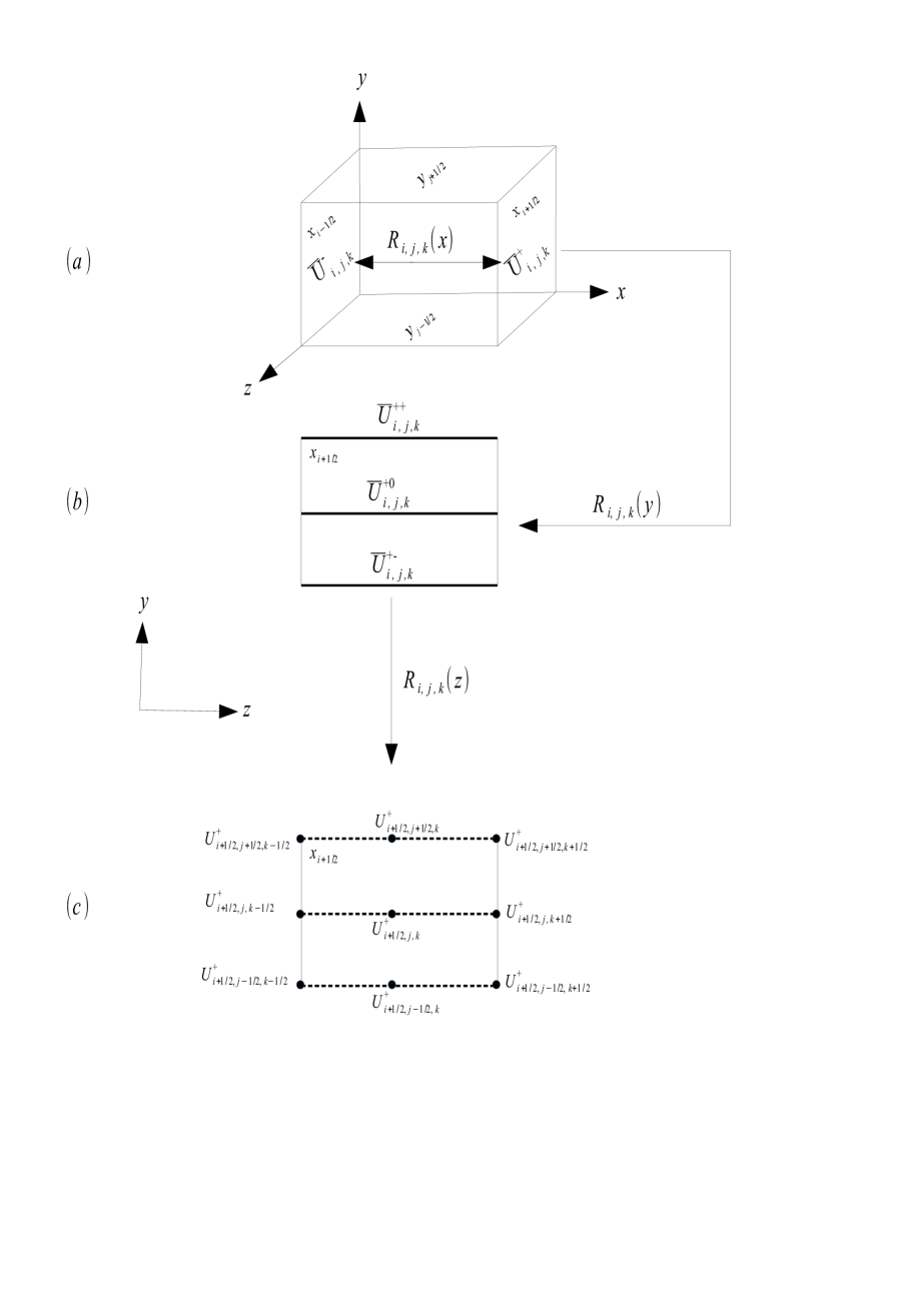
where $\rho$(A) is the maximum of the magnitude of the eigenvalues of the Jacobian matrix A. Although, this method has already been used by various authors in solving 2D problems (see for example Kurganov et al. (2001); Kurganov and Levy (2002); Balbás and Tadmor (2006); Cai et al. (2005)) using truly two-dimensional fourth order CWENO reconstruction, we are applying it dimension-by-dimension in solving 2D as well as 3D problems. Using the 1D CWENO reconstruction polynomial in the subsection A we first obtain area averages, ${\bf R}_{i,j,k}(x_{i\pm 1/2})=\overline{\bf U}_{i,j,k}^{\pm}$ at all the grid cell interfaces along the $x$-direction. Then we find new 1D CWENO polynomials ${\bf R}_{i,j,k}(y)$ based on those area averages by following the rules summarized in subsection A and adapted to the change from the $x$- to the $y$-direction. This allows to compute for each $x$-direction cell-interface three equidistant edge-averaged values along the $y$-direction, ${\bf R}_{i,j,k}(y_{j})=\overline{\bf U}_{i,j,k}^{+0}$ ($\overline{\bf U}_{i,j,k}^{-0}$), ${\bf R}_{i,j,k}(y_{j\pm 1/2})=\overline{\bf U}_{i,j,k}^{+{\pm}}$ ($\overline{\bf U}_{i,j,k}^{-{\pm}}$) - one in the face center and other two on the face boundaries, respectively. Afterwards, we find new 1D CWENO polynomials ${\bf R}_{i,j,k}(z)$ based on already computed edge-averaged values following subsection A and adapting to change from the $x$- to the $z$-direction. This allows, for each $x$-direction cell-interface, to compute three equidistant fourth-order accurate point values along the $z$-direction, one at the edge-center ${\bf R}_{i,j,k}(z_{k})$ and other two at the edge boundaries ${\bf R}_{i,j,k}(z_{k\pm 1/2})$. For example, point values corresponding to $z$-averaged values $\overline{\bf U}_{i,j,k}^{+0}$ are ${\bf R}_{i,j,k}(z_{k})={\bf U}_{i+1/2,j,k}^{+}$ and ${\bf R}_{i,j,k}(z_{k\pm 1/2})={\bf U}_{i+1/2,j,k\pm 1/2}^{+}$. Similarly, remaining point values at the grid cell interfaces along the $x$-direction can be obtained as shown in figure 1.

Thus, in each grid cell we obtain nine fourth order accurate point values (four at the edge corners, four at the edge centers and one at the face center as can be seen in figure 1) on both the grid cell interfaces along the $x$-direction. This allows us to obtain the corresponding fourth order accurate point value fluxes, ${\bf F^{x}(U^{\pm})}$ and hence the fourth order accurate point value LLF, ${\bf f^{x}}$, as computed in Eqs.(17)-(18) for example at ($x_{i+1/2},y_{j},z_{k}$). This enables the computation of fourth order accurate averaged fluxes $\overline{\bf F^{x}}$ at all the interfaces along the $x$-direction using Eq.III.2.

Computation of fourth order accurate averaged fluxes along the $y$- and $z$-direction is straightforward due to the simplicity of the dimension-by-dimension approach. For example, in order to compute higher order averaged fluxes along the $y$-direction, we first reconstruct a new CWENO polynomial ${\bf R}_{i,j,k}(y)$ by adapting to change in the direction from $x$ to $y$ in the subsection A and obtain area-averages, ${\bf R}_{i,j,k}(y_{j\pm 1/2})=\overline{\bf U}_{i,j,k}^{\pm}$ at all the grid cell interfaces along the $y$-direction. Later, these averages are used to reconstruct new 1D CWENO polynomials, ${\bf R}_{i,j,k}(z)$ again by adapting to change in the direction from $x$ to $z$ in the subsection A which allow the computation of three equidistant edge-averaged values along the $z$-direction, ${\bf R}_{i,j,k}(z_{k})=\overline{\bf U}_{i,j,k}^{+0}$ ($\overline{\bf U}_{i,j,k}^{-0}$), ${\bf R}_{i,j,k}(z_{k\pm 1/2})=\overline{\bf U}_{i,j,k}^{+{\pm}}$ ($\overline{\bf U}_{i,j,k}^{-{\pm}}$) - one in the face center and other two on the face boundaries, respectively. Based on these edge-averages new 1D CWENO polynomial ${\bf R}_{i,j,k}(x)$ is reconstructed so as to obtain corresponding point-values at the edge-centers ${\bf R}_{i,j,k}(x_{i})$ and edge boundaries ${\bf R}_{i,j,k}(x_{i\pm 1/2})$. Thus, we obtain nine fourth order accurate point values on both the grid cell interfaces along the $y$-direction in each grid cell and this allows us to obtain corresponding fourth order accurate point value fluxes, ${\bf F^{y}(U^{\pm})}$. Expression for the LLF, ${\bf f^{y}}$ at the face center ($x_{i},y_{j+1/2},z_{k}$) can be obtained by adapting to change in the direction from $x$ to $y$ in Eq.(17) as follows,

$${\bf f^{y}}_{i,j+1/2,k}=\frac{{\bf F^{y}}({\bf U}_{i,j+1/2,k}^{-})+{\bf F^{y}}({\bf U}_{i,j+1/2,k}^{+})}{2}-\\ \frac{a^{y}_{i,j+1/2,k}}{2}({\bf U}^{-}_{i,j+1/2,k}-{\bf U}^{+}_{i,j+1/2,k})\,,$$ (19)

where the quantities ${\bf U}_{i,j+1/2,k}^{+}$ and ${\bf U}_{i,j+1/2,k}^{-}$ are the fourth order accurate point values computed from the area averages ${\bf R}_{i,j,k}(y_{j+1/2})$ and ${\bf R}_{i,j+1,k}(y_{j-1/2})$, respectively and ${\bf F^{y}}({\bf U}_{i,j+1/2,k}^{+})$, ${\bf F^{y}}({\bf U}_{i,j+1/2,k}^{-})$ are the respective point value fluxes. And the quantity $a^{y}$ is the local maximum speeds of propagation which is estimated as,

$$a^{y}_{i,j+1/2,k}=\text{max}\left\{\rho\left(\frac{\partial{\bf F^{y}}({\bf U}_{i,j+1/2,k}^{+})}{\partial U}\right),\\ \rho\left(\frac{\partial{\bf F^{y}}({\bf U}_{i,j+1/2,k}^{-})}{\partial U}\right)\right\}\,,$$ (20)

where $\rho$(A) is the maximum of the magnitude of the eigenvalues of the Jacobian matrix A. Similarly, remaining point value LLF along the $y$-direction can be obtained. Now the expression for the fourth order accurate averaged flux along the $y$-direction can also be obtained by adapting to change from $x$- to $y$-direction in Eq.(III.2) as,

$$\overline{\bf F^{y}}_{i,j\pm 1/2,k}=\frac{1}{36}\Big{\{}{\bf f^{y}}_{i-1/2,j\pm 1/2,k-1/2}+4{\bf f^{y}}_{i-1/2,j\pm 1/2,k}+{\bf f^{y}}_{i-1/2,j\pm 1/2,k+1/2}$$

$$+4({\bf f^{y}}_{i,j\pm 1/2,k-1/2}+4{\bf f^{y}}_{i,j\pm 1/2,k}+{\bf f^{y}}_{i+1/2,j\pm 1/2,k})$$

$$+{\bf f^{y}}_{i+1/2,j\pm 1/2,k-1/2}+4{\bf f^{y}}_{i+1/2,j\pm 1/2,k}+{\bf f^{y}}_{i+1/2,j\pm 1/2,k+1/2}\Big{\}}+{\bf\mathcal{O}}(\Delta x^{4}+\Delta z^{4})$$ (21)

Thus, from Eq.(III.2) we obtain the fourth order accurate averaged flux, $\overline{\bf F^{y}}$, at all the interfaces along the $y$-direction. Similarly, fourth order accurate averaged flux along the $z$-direction, $\overline{\bf F^{z}}$ can be easily obtained following the above described method . After computing fourth order accurate averaged fluxes ($\overline{\bf F^{x}}$,$\overline{\bf F^{y}}$,$\overline{\bf F^{z}}$), Eq.(3) is evolved using a classical fourth order accurate low-storage Runge-Kutta method Williamson (1980) in order to achieve fourth order accuracy during the temporal evolution and the steps are explained as follows: let us assume that R.H.S. of Eq.(3) is ${\bf C[\overline{U}_{i,j,k}]}$, now dropping the subscripts $(i,j,k)$ Eq.(3) can be rewritten as,

$$\frac{d\overline{\bf U}(t)}{dt}={\bf C}[{\bf\overline{U}}(t)]$$ (22)

The intermediate steps to solve Eq.(22) are as follows,

$${\bf K}_{1}={\bf C}[{\bf\overline{U}}(t_{n})],$$

$$\overline{\bf U}_{1}={\bf\overline{U}}(t_{n})+\frac{\Delta t}{2}{\bf K}_{1},$$

$${\bf K}_{2}={\bf C}[{\bf\overline{U}}_{1}],$$

$$\overline{\bf U}_{2}={\bf\overline{U}}(t_{n})+\frac{\Delta t}{2}{\bf K}_{2},$$

$${\bf K}_{3}={\bf C}[{\bf\overline{U}}_{2}],$$

$$\overline{\bf U}_{3}={\bf\overline{U}}(t_{n})+{\Delta t}{\bf K}_{3},$$

$${\bf K}_{4}={\bf C}[{\bf\overline{U}}_{3}],$$

$$\overline{\bf U}(t_{n+1})={\bf\overline{U}}(t_{n})+\frac{\Delta t}{6}({\bf K}_{1}+2{\bf K}_{2}+2{\bf K}_{3}+{\bf K}_{4}).$$

Here, $n=0,1,2,3,....$ and ${\Delta t}$ is determined dynamically according to the Courant-Friedrichs-Lewy (CFL) constraint (see for example, Núñez-De La Rosa and Munz (2016)),

$$\Delta t=C_{CFL}min\left(\frac{\Delta x}{a^{x}_{max}},\frac{\Delta y}{a^{y}_{max}},\frac{\Delta z}{a^{z}_{max}}\right),$$ (23)

where, $C_{CFL}$ is the CFL number which for all the 3D tests is chosen as, $0.3$ and for all the 2D tests as, $0.45$. The quantities $a^{x}_{max}$, $a^{y}_{max}$ and $a^{z}_{max}$ are the maximum values of $a^{x}_{i+1/2,j,k}$, $a^{y}_{i,j+1/2,k}$ and $a^{z}_{i,j,k+1/2}$, respectively for all $(i,j,k)$.

Tests with a modern strongly stability preserving Runge-Kutta scheme of fourth order Ketcheson (2008) have not displayed significant improvements of accuracy but of course increases overall performance by allowing larger timesteps.

We have confirmed the fourth order accuracy and the shock capturing nature of this method in various nonlinear multidimensional problems. However, this method turns out to be computationally too expensive for 3D problems as it requires seventy eight sweeps of 1D CWENO reconstruction in each grid cell.

Method B – One way of reducing the number of computationally expensive reconstruction steps is to compute the averaged flux (say along the $x$-direction) as follows,

$${\bf\overline{F}^{x}}_{i\pm 1/2,j,k}={\bf f^{x}}_{i\pm 1/2,j,k}+\frac{1}{24}({\bf f^{x}}_{i\pm 1/2,j-1,k}-2{\bf f^{x}}_{i\pm 1/2,j,k}+{\bf f^{x}}_{i\pm 1/2,j+1,k})$$

$$+\frac{1}{24}({\bf f^{x}}_{i\pm 1/2,j,k-1}-2{\bf f^{x}}_{i\pm 1/2,j,k}+{\bf f^{x}}_{i\pm 1/2,j,k+1})+{\bf\mathcal{O}}(\Delta y^{4}+\Delta z^{4}).$$ (24)

This approximation to the averaged flux can be obtained from Eq.(III.1) by replacing ${\bf R}_{i,j,k}(x_{i\pm 1/2})$ (area-average quantity) with ${\bf\overline{F}^{x}}_{i\pm 1/2,j,k}$, ${{\bf U}}(x_{i\pm 1/2},y_{j},z_{k})$ (point value at the face-center) with ${\bf f^{x}}_{i\pm 1/2,j,k}$ and second order derivatives along the $y$- and $z$-directions are approximated by finite difference formula for point values at the face-center. Thus, in this method as opposed to Eq.(III.2) we just need to obtain point values at the face centers. This averaging procedure has previously been used to obtain higher order averaged flux in the multidimensional PPM (piecewise parabolic method) McCorquodale and Colella (2011) and WENO schemes Buchmüller and Helzel (2014). Whereas, we are applying it in the framework of a central scheme which naturally allows the computation of non-oscillatory point values (${\bf U}_{i+1/2,j,k}^{+}$, ${\bf U}_{i-1/2,j,k}^{-}$) at the face-center. The procedure for computing fourth order accurate point values at the face-centers and the corresponding point value LLF (Eq.(17)) is already described for method A. Once we know the point value LLF fluxes at the face centers, ${\bf f^{x}}_{i\pm 1/2,j,k}$, the averaged fluxes along the $x$-direction, ${\bf\overline{F}^{x}}_{i\pm 1/2,j,k}$ can straightforwardly be obtained from Eq.(III.2). The expression for the fourth order accurate averaged flux along the $y(z)$-direction, $\overline{\bf F^{y}}(\overline{\bf F^{z}})$, can be obtained by adapting to the change from the $x$-direction to the $y(z)$-direction in Eq.(III.2). After the computation of the fourth order accurate averaged fluxes ($\overline{\bf F^{x}}$,$\overline{\bf F^{y}}$,$\overline{\bf F^{z}}$), Eq.(3) is evolved using a fourth order accurate Runge-Kutta method as described for method A.

We have confirmed the fourth order accuracy and the shock capturing nature of this procedure as well in various nonlinear multidimensional problems. Moreover, this method turns out to be computationally lesser expensive as it requires only twelve sweeps of 1D CWENO reconstruction in each grid cell for 3D problems.

Method C – one can further reduce the computational cost by obtaining the fourth order accurate point value at the face center as follows,

$${{\bf U}}_{i+1/2,j,k}^{+}=\overline{\bf U}_{i,j,k}^{+}-\frac{1}{24}(\overline{\bf U}_{i,j-1,k}^{+}-2\overline{\bf U}_{i,j,k}^{+}+\overline{\bf U}_{i,j+1,k}^{+})$$

$$-\frac{1}{24}(\overline{\bf U}_{i,j,k-1}^{+}-2\overline{\bf U}_{i,j,k}^{+}+\overline{\bf U}_{i,j,k+1}^{+})+{\bf\mathcal{O}}(\Delta y^{4}+\Delta z^{4}).$$ (25)

This expression can also be derived from Eq.(III.1) by replacing ${\bf R}_{i,j,k}(x_{i+1/2})$ (area-average quantity) with ${\bf\overline{U}}_{i,j,k}^{+}$, ${{\bf U}}(x_{i+1/2},y_{j},z_{k})$ (point value at the face-center) with ${\bf U}_{i+1/2,j,k}^{+}$ and by approximating second order derivatives along the $y$- and $z$-directions using the finite difference formula for area-averages, ${\bf\overline{U}}_{i,j,k}^{+}$. Similarly, one can obtain the point value at the center of the opposite interface, ${\bf U}_{i-1/2,j,k}^{-}$ by replacing $\overline{\bf U}_{i,j,k}^{+}$ with $\overline{\bf U}_{i,j,k}^{-}$ and ${{\bf U}}_{i+1/2,j,k}^{+}$ with ${{\bf U}}_{i-1/2,j,k}^{-}$ in Eq.(III.2) as,

$${{\bf U}}_{i-1/2,j,k}^{-}=\overline{\bf U}_{i,j,k}^{-}-\frac{1}{24}(\overline{\bf U}_{i,j-1,k}^{-}-2\overline{\bf U}_{i,j,k}^{-}+\overline{\bf U}_{i,j+1,k}^{-})$$

$$-\frac{1}{24}(\overline{\bf U}_{i,j,k-1}^{-}-2\overline{\bf U}_{i,j,k}^{-}+\overline{\bf U}_{i,j,k+1}^{-})+{\bf\mathcal{O}}(\Delta y^{4}+\Delta z^{4}).$$ (26)

This method of computing higher-order point value at the face-center has previously been used in the framework of the third order CWENO scheme of Kurganov and Levy Kurganov and Levy (2000), fourth order PPM scheme McCorquodale and Colella (2011) and fourth order WENO scheme Buchmüller and Helzel (2014). We are applying this method to develop a fourth-order accurate CWENO scheme. The expressions for the fourth-order accurate point values at the face-centers along the $y(z)$-direction can be obtained from Eqs.(III.2)-(III.2) by adapting to the change from $x$-direction to $y(z)$-direction. Once the point values at all the face-centers are computed, averaged fluxes ($\overline{\bf F^{x}}$,$\overline{\bf F^{y}}$,$\overline{\bf F^{z}}$) are obtained as described for method A. The temporal evolution of Eq.(3) is same as described for method A.

We have compared the accuracy, non-oscillatory behavior and computational expense of all the three methods for various multi-dimensional nonlinear problems and found no significant difference among the three except the computational cost.

In TABLE 1, we compare the performance of the three methods for 3D linear advection test and find that the method C is approximately $4.3$ times faster than method A and $1.87$ times faster than method B.

NG	Method C	Method A	Method B
$32^{3}$	1.0	6.06	1.87
$64^{3}$	1.0	3.57	1.93
$128^{3}$	1.0	3.46	1.88
$256^{3}$	1.0	3.32	1.95
$512^{3}$	1.0	5.09	1.72
Mean	1.0	4.3	1.87

Table 1: Performance test for the three methods where the run time is normalized with respect to method C

Since method C seems to be the most efficient in terms of computational cost, therefore, in this manuscript we will show robustness of this method by solving various multidimensional problems. Please note here that although with this method we do not encounter the problem of negative pressure or density in any of the tests while solving Euler equations, it can not be ruled out that strong discontinuities may introduce such unphysical effects. Therefore, we recommend to check for the positivity of density and pressure after the computation of point values in Eqs.(III.2)-(III.2) and switch off the addition of approximated derivatives when the check fails. Thus, in such situations the point value at the face center, ${{\bf U}}_{i+1/2,j,k}^{+}$ is replaced by its second order approximation, ${\overline{\bf U}}_{i,j,k}^{+}$.

It is to note here that 3D hyperbolic equations reduce to 2D hyperbolic equations when there are no variations along the $z$-direction. Therefore, a 2D hyperbolic equation is a simpler version of a 3D equation (1) which can be obtained by dropping the variations along the $z$-direction i.e., the fourth term $(\frac{\partial\bf F^{z}}{\partial z})$ in Eq.(1). Thus, in 2D problems volume-averaged quantities ($say,\overline{\bf U}_{i,j,k}$) would reduce to area-averages ($\overline{\bf U}_{i,j}$) and area-averaged quantities ($say,\overline{\bf F^{x}}_{i\pm 1/2,j,k}$) would reduce to edge-averages $(\overline{\bf F^{x}}_{i\pm 1/2,j})$. So, the discretization and the numerical schemes for 2D problems can be recovered just by dropping the variation along the $z$-direction as well as the subscripts “$k,k\pm$” in all the expression throughout the paper.

The code is MPI (message-passing-interface) parallel, using a two-dimensional decomposition of the computational grid. The 2D decomposition is also referred to as the pencil decomposition or column decomposition. It is used when the number of processes comes close to, or even exceeds, the number of grid cells in one spatial dimension. In two of the three space dimensions the grid is divided and distributed over the processes. The third dimension resides entirely within each process. All tests have been performed on a parallel architecture based on Intel Xeon ‘Sandybridge’ cpus.

IV Accuracy

In this section, we present the convergence of errors by solving the Euler equations of gas dynamics. We first extract the 1D profile of a physical quantity from the 2D (or 3D) grid and then the norm of the error for all the convergence studies can be computed as follows,

$$L_{1}=\frac{1}{NG}\sum_{i=1}^{NG}|E_{i}^{f}-E_{i}^{0}|,$$ (27)

where $E_{i}^{0}$, $E_{i}^{f}$ are the exact reference and the numerical solutions as a function of grid resolution and $NG$ is the number of grid points.

After computing the norms of the errors, we obtain the experimental order of convergence $(EOC)$ using the formula,

$$EOC(j)=\frac{|log(L_{1}(NG(j)))|-|log(L_{1}(NG(j-1)))|}{|log(NG(j))|-|log(NG(j-1))|},$$ (28)

here $j$ runs over the indices of the column vectors in the tables shown in the later subsections.

IV.1 The Euler Equations of Gas Dynamics

Equations governing the dynamics of a 3D adiabatic system can be described by Eq.(1) where,

$${\bf U}=\left(\begin{array}[]{c}\rho\\ \rho v_{x}\\ \rho v_{y}\\ \rho v_{z}\\ E\end{array}\right),\hskip 5.69046pt{\bf F^{x}}=\left(\begin{array}[]{c}\rho v_{x}\\ \rho v_{x}^{2}+p\\ \rho v_{x}v_{y}\\ \rho v_{x}v_{z}\\ v_{x}(E+p)\end{array}\right),\hskip 5.69046pt{\bf F^{y}}=\left(\begin{array}[]{c}\rho v_{y}\\ \rho v_{x}v_{y}\\ \rho v_{y}^{2}+p\\ \rho v_{y}v_{z}\\ v_{y}(E+p)\end{array}\right),\hskip 5.69046pt{\bf F^{z}}=\left(\begin{array}[]{c}\rho v_{z}\\ \rho v_{x}v_{z}\\ \rho v_{y}v_{z}\\ \rho v_{z}^{2}+p\\ v_{z}(E+p)\end{array}\right).$$ (49)

Here $\rho$ is the density, $v_{x}$, $v_{y}$, $v_{z}$ are $x$, $y$ and $z$ component of the velocity, $E$ is the total energy and $p$ is the pressure which is related to $E$ through $p=(\gamma-1)(E-0.5\rho(v_{x}^{2}+v_{y}^{2}+v_{z}^{2}))$. One may recover 2D adiabatic systems just by dropping the $z$ components from Eq. (49). Boundary conditions are periodic.

IV.1.1 Linear Problems

$Example$ $1.$ The initial conditions, for the 2D and 3D cases, are chosen as follows:

$$\rho(x,y,0)=1+0.5\sin[2\pi(x/l_{x}+y/l_{y})],$$

$$v_{x}(x,y,0)=1=v_{y}(x,y,0),$$

$$p(x,y,0)=3/5,\hskip 5.69046ptl_{x}\times l_{y}=[0,1]\times[0,1].$$

$$\rho(x,y,z,0)=1+0.5\sin[2\pi(x/l_{x}+y/l_{y}+z/l_{z})],$$

$$v_{x}(x,y,z,0)=1.0=v_{y}(x,y,z,0)=v_{z}(x,y,z,0),$$

$$p(x,y,z,0)=3/5,\hskip 5.69046ptl_{x}\times l_{y}\times l_{z}=[0,1]\times[0,1]\times[0,1].$$

Here $\gamma$ is chosen to be $5/3$ and the numerical solutions are obtained after one period. These initial conditions result in the advection of the initial density profile due to constant velocity components and constant pressure (see for example Buchmüller and Helzel (2014)). TABLE 2 and TABLE 3 contain the convergence of errors for the 2D and 3D linear Euler gas dynamics, respectively.

j	NG	$L_{1}$	EOC
1	$16^{2}$	1.209E-3	-
2	$32^{2}$	4.367E-5	4.79
3	$64^{2}$	1.616E-6	4.75
4	$128^{2}$	7.413E-8	4.44
5	$256^{2}$	4.075E-9	4.18

Table 2: Convergence of errors for the 2D linear Euler gas dynamics

j	NG	$L_{1}$	EOC
1	$16^{3}$	4.793E-3	-
2	$32^{3}$	1.753E-4	4.77
3	$64^{3}$	6.389E-6	4.77
4	$128^{3}$	2.876E-7	4.47
5	$256^{3}$	1.637E-8	4.13

Table 3: Convergence of errors for the 3D linear Euler gas dynamics

IV.1.2 Nonlinear Problems

$Example$ $2.$ Initial conditions for the 2D Euler vortex evolution problem (see for example Hu and Shu (1999)) are,

$$\left(\begin{array}[]{c}\rho\\ v_{x}\\ v_{y}\\ p\end{array}\right)=\left(\begin{array}[]{c}(1+\delta T)^{1/(\gamma-1)}\\ 1+(l_{y}/2-y)\frac{\sigma}{2\pi}e^{0.5(1-r^{2})}\\ 1+(x-l_{x}/2)\frac{\sigma}{2\pi}e^{0.5(1-r^{2})}\\ (1+\delta T)^{\gamma/(\gamma-1)}\end{array}\right),$$ (58)

Here $\delta T$ is the perturbation in the temperature and is given by,

$$\delta T=-\frac{(\gamma-1)\sigma^{2}}{8\gamma\pi^{2}}e^{(1-r^{2})},$$

where $r^{2}=(x-l_{x}/2)^{2}+(y-l_{y}/2)^{2}$ and the vortex strength $\sigma$ = 5, $l_{x}\times l_{y}=[0,10]\times[0,10]$. Here $\gamma$ is chosen to be $1.4$. The initial conditions lead advection of a non-linear vortex at an angle of $45^{\circ}$ with the $x$-axis and the numerical solutions are obtained after one period ($t=10$). Convergence of errors for this nonlinear problem are presented in TABLE 4.

j	NG	$L_{1}$	EOC
1	$32^{2}$	6.584E-3	-
2	$96^{2}$	5.255E-5	4.39
3	$160^{2}$	4.449E-6	4.83
4	$288^{2}$	2.757E-7	4.73

Table 4: 2D vortex evolution problem

$Example$ $3.$ Euler equations with the initial conditions (see for example Buchmüller and Helzel (2014)),

$$\rho(x,y,0)=1+0.5\sin[\pi(x+y-2)],$$

$$v_{x}(x,y,0)=\cos[\pi(x+2y-3)],v_{y}(x,y,0)=1-0.5\sin[\pi(2x+y-3)],$$

$$p(x,y,0)=1-0.5\sin[\pi(x-y)],\hskip 5.69046ptl_{x}\times l_{y}=[0,2]\times[0,2].$$

follow the nonlinear evolution and lead to discontinuous solution after a finite time. Here $\gamma$ is chosen to be $1.4$ and the numerical solutions are obtained at $t=0.05$ (solution is still smooth) and the reference solution is obtained at high resolution $(1056\times 1056)$. Convergence of errors for this nonlinear problem are shown in TABLE 5.

j	NG	$L_{1}$	EOC
1	$32^{2}$	4.686E-4	-
2	$96^{2}$	6.068E-6	3.96
3	$160^{2}$	4.459E-7	5.11
4	$288^{2}$	2.821E-8	4.69

Table 5: 2D nonlinear Euler problem

IV.2 Comparison with truly multidimensional CWENO schemes

In this section we compare the convergence of errors for the 3D linear advection test and 3D Burgers’ equation with a truly 3D central scheme Lahooti and Pishevar (2012).

$Example$ $4.$ Three dimensional linear advection test –

Equation for the 3D linear advection test is,

$$\frac{\partial U}{\partial t}+\frac{\partial U}{\partial x}+\frac{\partial U}{\partial y}+\frac{\partial U}{\partial z}=0,$$

and the initial condition is chosen to be,

$$U(x,y,z)=\sin^{2}(\pi x)\sin^{2}(\pi y)\sin^{2}(\pi z).$$

Computational domain is a unit cube, i.e., $l_{x}\times l_{y}\times l_{z}=[0,1]\times[0,1]\times[0,1]$ and the boundary conditions are periodic. Thus, all the parameters for this test are chosen to be same as in ref. Lahooti and Pishevar (2012). In the TABLE 6 we provide a comparison for the error norm,

j		dim-by-dim		3D CWENO
	NG	$L_{1}$	EOC	$L_{1}$	EOC
1	$10^{3}$	2.252E-2	-	1.08E-2	-
2	$20^{3}$	9.728E-4	4.53	6.395E-4	4.09
3	$40^{3}$	4.024E-5	4.59	3.834E-5	4.06
4	$80^{3}$	1.875E-6	4.42	2.3633E-6	4.02

Table 6: 3D linear advection test

$Example$ $5.$ Three dimensional Burgers’ equation –

Equation for the 3D Burgers’ equation is expressed as follows,

$$\frac{\partial U}{\partial t}+\frac{\partial}{\partial x}\Big{(}\frac{U^{2}}{2}\Big{)}+\frac{\partial}{\partial y}\Big{(}\frac{U^{2}}{2}\Big{)}+\frac{\partial}{\partial z}\Big{(}\frac{U^{2}}{2}\Big{)}=0,$$

and the initial condition is chosen to be,

$$U(x,y,z)=0.25+\sin(\pi x)\sin(\pi y)\sin(\pi z).$$

Computational domain is chosen as, $l_{x}\times l_{y}\times l_{z}=[-1,1]\times[-1,1]\times[-1,1]$ and the boundary conditions are periodic. Thus, all the parameters for this test also are chosen to be same as in ref. Lahooti and Pishevar (2012). The only difference is that we obtain the reference solution by evolving the equation at high resolution ($510^{3}$). In the TABLE 7 we provide a comparison for $L_{1}$ error norm,

j	dim-by-dim			3D CWENO
	NG	$L_{1}$	EOC	NG	$L_{1}$	EOC
1	$10^{3}$	4.005E-3	-	$10^{3}$	6.846E-3	-
2	$30^{3}$	5.915E-5	3.84	$20^{3}$	5.804E-4	3.56
3	$50^{3}$	6.692E-6	4.27	$40^{3}$	3.347E-5	4.16
4	$90^{3}$	5.079E-7	4.39	$80^{3}$	1.766E-6	4.21

Table 7: 3D Burgers’ equation

V Non-oscillatory behavior

In this section we present solutions for the oblique Sod’s shock tube problem, the oblique Lax problem, the 2D blast wave, the 2D Riemann problem, the 3D Burgers’ equation and the 3D blast wave problem to demonstrate the non-oscillatory behavior and compare the results with genuine multi-dimensional fourth order accurate central schemes Levy et al. (2002); Lahooti and Pishevar (2012). Moreover, well known and more realistic problems like Kelvin-Helmholtz instability Price (2008) and shock-bubble interaction Holden et al. (1999); Langseth and LeVeque (2000) problems are also solved to demonstrate the robustness of the scheme.

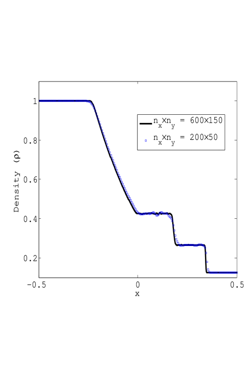
The oblique Sod’s shock tube problem – We solve the Euler gas dynamics, described in Eq.(49), for a 1D shock tube initial value problem Sod (1978) on 2D grid such that the initial discontinuity makes an angle of $60^{\circ}$ with the $x$-axis. Initial condition for this test are chosen to be same as in ref. Levy et al. (2002) and can be expressed as,

$$\left(\begin{array}[]{c}\rho\\ v_{x}\\ v_{y}\\ p\end{array}\right)_{L}=\left(\begin{array}[]{c}1\\ 0\\ 0\\ 1\end{array}\right),\hskip 22.76228pt\left(\begin{array}[]{c}\rho\\ v_{x}\\ v_{y}\\ p\end{array}\right)_{R}=\left(\begin{array}[]{c}0.125\\ 0\\ 0\\ 0.1\end{array}\right),$$ (75)

In this test $\gamma$ is chosen to be $1.4$. The computational domain is the rectangle, $l_{x}\times l_{y}=[-0.5,0.5]\times[-0.125,0.125]$ and boundary conditions are open. The solution is sampled at $y=0.0$ at time $t=0.16632$. In figure 2, we compare the solutions at two different resolutions $[200\times 50]$ and $[600\times 150]$. At the coarser resolution $[200\times 50]$, we see some small amplitude wiggles, near the contact discontinuity (also observed in reference Levy et al. (2002)) which gets smaller at a finer resolution $[600\times 150]$.

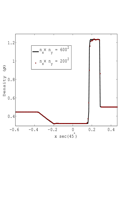
The oblique Lax problem – In this problem we again solve the Euler gas dynamics, described in Eq.(49), on the 2D grid such that the initial discontinuity makes an angle of $45^{\circ}$ with the $x$-axis and the initial conditions are expressed as,

$$\left(\begin{array}[]{c}\rho\\ v_{x}\\ v_{y}\\ p\end{array}\right)_{L}=\left(\begin{array}[]{c}0.445\\ 0.698/\sqrt{2}\\ 0.698/\sqrt{2}\\ 3.528\end{array}\right),\hskip 22.76228pt\left(\begin{array}[]{c}\rho\\ v_{x}\\ v_{y}\\ p\end{array}\right)_{R}=\left(\begin{array}[]{c}0.5\\ 0\\ 0\\ 0.571\end{array}\right).$$ (92)

Here $\gamma$ is chosen to be $1.4$, computational domain as, $l_{x}\times l_{y}=[-0.5,0.5]\times[-0.5,0.5]$ and boundary conditions are open. In figure 3, two solutions at the resolutions $200^{2}$ and $600^{2}$ are compared at time $t=0.12$ and in this test also it is found that, small amplitude wiggles near the contact discontinuity get smaller at a finer resolution and get further smaller with time.

Please note here that changing the time integrator for example low storage strong stability-preserving Runge-Kutta method Ketcheson (2008) does not affect the amplitude of the wiggles.

The 2D blast wave problem – Here we solve Eq.(49) for the same initial condition as in Levy et al. (2002) which can be expressed as follows,

$$\left(\begin{array}[]{c}\rho,v_{x},v_{y},p\end{array}\right)=\left\{\begin{array}[]{c}(1,0,0,1)\hskip 5.69046pt\text{if}\hskip 5.69046pt(x-l_{x}/2)^{2}+(y-l_{y}/2)^{2}\leq R^{2}\\ (0.125,0,0,0.1)\hskip 5.69046pt\text{otherwise}\end{array}\right\}.$$ (96)

Here $R=0.2$, $\gamma$ = $1.4$, the boundary conditions are periodic and the computational domain is chosen as, $l_{x}\times l_{y}=[0,1]\times[0,1]$. We compare the solutions, at time $t=0.1$ at grid resolutions $100^{2}$ and $200^{2}$, shown in figure 4 and figure 5, respectively. From these figures it becomes clear that our scheme in spite of being so simple produces results which are very close to truly multidimensional CWENO scheme Levy et al. (2002) as the symmetry loss gets better at higher resolution. Probably, using more accurate numerical flux (HLL, see for example Capdeville (2011)) may reduce the symmetry loss.

The 2D Riemann problem – In this test, we solve Eq.(49) for configuration $5$ of ref.Kurganov and Tadmor (2002) which is also used in ref.Levy et al. (2002), so the initial conditions are chosen as,

$$\left(\begin{array}[]{c}\rho,v_{x},v_{y},p\end{array}\right)=\left\{\begin{array}[]{c}(1,-0.75,-0.5,1)\hskip 5.69046pt\text{if}\hskip 5.69046ptx>0,y>0\\ (2,-0.75,0.5,1)\hskip 5.69046pt\text{if}\hskip 5.69046ptx<0,y>0\\ (1,0.75,0.5,1)\hskip 5.69046pt\text{if}\hskip 5.69046ptx<0,y<0\\ (3,0.75,-0.5,1)\hskip 5.69046pt\text{if}\hskip 5.69046ptx>0,y<0\end{array}\right\}.$$ (102)

Here $\gamma$ = $1.4$, the boundary conditions are open and the computational domain is chosen as, $l_{x}\times l_{y}=[-0.5,0.5]\times[-0.5,0.5]$. This configuration results in four interacting contact discontinuities. The solutions are obtained at $t=0.23$ at two different grid resolutions $200^{2}$ and $400^{2}$ shown in figure 6 and figure 7, respectively. For the adiabatic system considered here, the obtained solution is not expected to be symmetric about the oirigin Schulz-Rinne et al. (1993). This test displays the scheme’s ability to correctly handle the partly intricate structuring in spite of the method’s comparable simplicity.

The 3D Burgers’ equation – The problem of the 3D Burgers’ equation is already described in $Example$ $5$ and solutions are obtained at time $t=0.8$. Figure 8 and figure 9 show the contour plots at resolutions $80^{3}$ (same as in ref.Lahooti and Pishevar (2012)) and $400^{3}$, respectively in the plane $z=0$.

The 3D blast (explosion) test problem – In this problem we solve 3D Euler equation [Eq.(49)] for the same initial conditions as used in ref. Lahooti and Pishevar (2012) which are expressed as follows,

$$\left(\begin{array}[]{c}\rho,v_{x},v_{y},v_{z},p\end{array}\right)=\left\{\begin{array}[]{c}(1,0,0,0,1)\hskip 5.69046pt\text{if}\hskip 5.69046pt(x-l_{x}/2)^{2}+(y-l_{y}/2)^{2}+(z-l_{z}/2)^{2}\leq R^{2}\\ (0.125,0,0,0,0.1)\hskip 5.69046pt\text{otherwise}\end{array}\right\}.$$ (106)

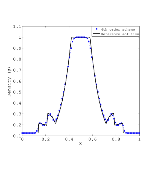
Here $R=0.2$, $\gamma$ = $1.4$, the boundary conditions are periodic and the computational domain is unit-cube, $l_{x}\times l_{y}\times l_{z}=[0,1]\times[0,1]\times[0,1]$. Solutions are obtained at $t=0.1$. Figure 10 shows the 1D profile of the density $(\rho)$, obtained along the intersection of planes $y=0.5$ and $z=0.5$ at a resolution $80^{3}$ (same as in ref.Lahooti and Pishevar (2012)) and the reference solution is obtained at a high resolution $720^{3}$.

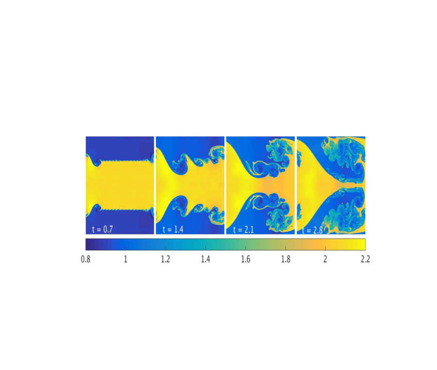
Kelvin-Helmholtz (KH) instability – In this problem we solve Eq.(49) in 2D along with periodic boundary conditions and the computational domain is set as, $l_{x}\times l_{y}=[-0.5,0.5]\times[-0.5,0.5]$. The pressure is in equilibrium with $p=2.5$ everywhere and $\gamma=5/3$. Here the problem is initialized as suggested in ref. Price (2008), so the initial conditions can be expressed as,

$$\left(\begin{array}[]{c}\rho,v_{x},v_{y},p\end{array}\right)=\left\{\begin{array}[]{c}(2,0.5,0,2.5)\hskip 5.69046pt\text{if}\hskip 5.69046pt|y|<0.25\\ (1,-0.5,-0.025\sin[2\pi(x+0.5)/\lambda],2.5)\hskip 5.69046pt\text{if}\hskip 5.69046pt|y-0.25|<0.025\\ (1,-0.5,0.025\sin[2\pi(x+0.5)/\lambda],2.5)\hskip 5.69046pt\text{if}\hskip 5.69046pt|y+0.25|<0.025\\ (1,-0.5,0,2.5)\hskip 5.69046pt\text{elsewhere }\end{array}\right\}.$$ (112)

Here, wavelength of the perturbation, $\lambda$ is chosen to be $6$. Figure 11 shows the snap-shots of color-coded contour plots for the density at time $t=0.7,1.4,2.1,2.8$ at a resolution $1024^{2}$. Generation of small scale structures during the nonlinear development of the KH instability are symmetrically captured.

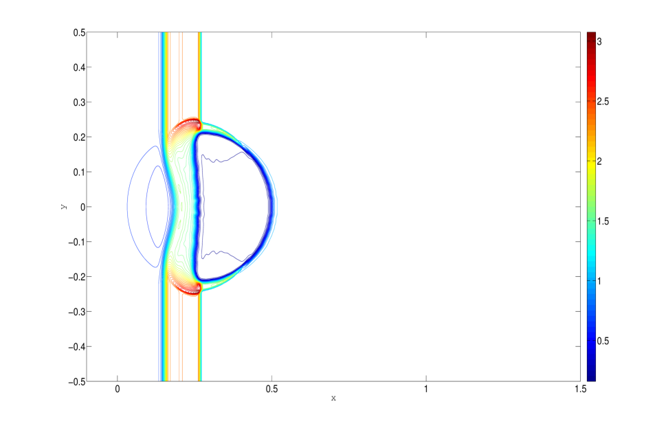
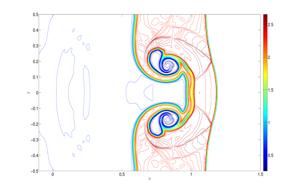
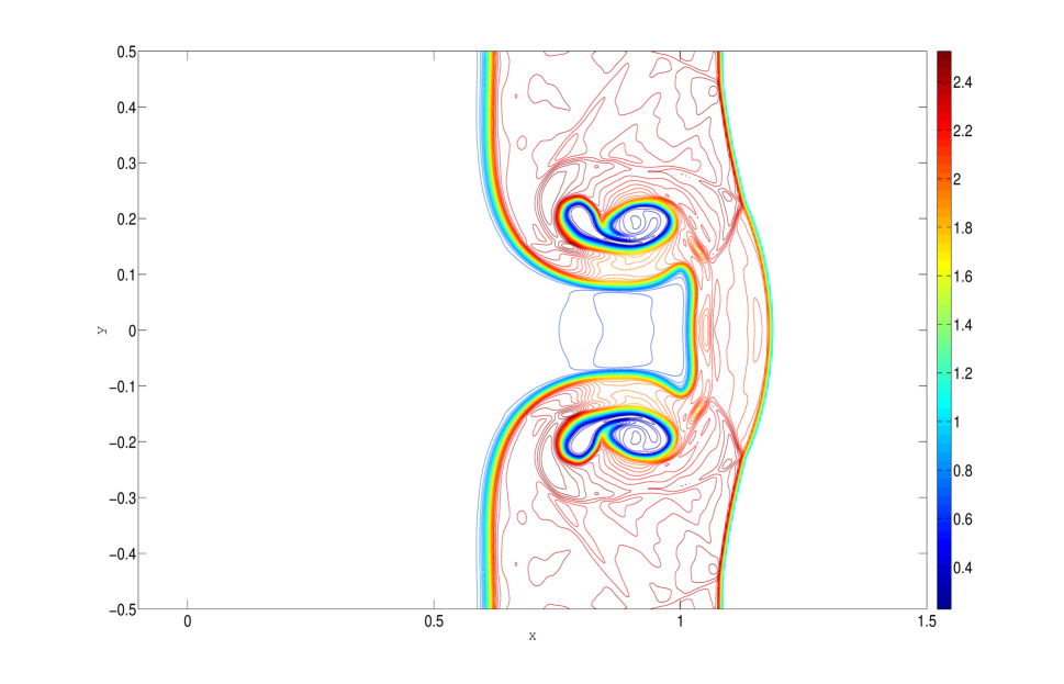
Shock-Bubble Interaction – In this test, Eq.(49) is solved to show the interaction of a planar shock with a low density circular region for the 2D test Holden et al. (1999) and with low density spherical region for the 3D test Langseth and LeVeque (2000). The computational domain for the 2D and 3D cases are chosen as, $l_{x}\times l_{y}=[-0.1,1.5]\times[-0.5,0.5]$ with resolution $400^{2}$ and $l_{x}\times l_{y}\times l_{z}=[-0.1,1.5]\times[-0.5,0.5]\times[-0.5,0.5]$ with resolution $400^{3}$, respectively. Boundary conditions are open and $\gamma=1.4$ in both the tests. Initial conditions for 2D and 3D tests are given by Eq.(117) and Eq.(122), respectively as,

$$\left(\begin{array}[]{c}\rho,v_{x},v_{y},p\end{array}\right)=\left\{\begin{array}[]{c}(1,0,0,1)\hskip 11.38092pt\text{if}\hskip 5.69046ptx>0\hskip 5.69046pt\text{and}\hskip 5.69046pt(x-0.3)^{2}+y^{2}\geq R^{2}\\ (1,0,0,10)\hskip 5.69046pt\text{if}\hskip 5.69046ptx<0\\ (0.1,0,0,1)\hskip 5.69046pt\text{otherwise}\end{array}\right\}.$$ (117)

$$\left(\begin{array}[]{c}\rho,v_{x},v_{y},v_{z},p\end{array}\right)=\left\{\begin{array}[]{c}(1,0,0,0,1)\hskip 11.38092pt\text{if}\hskip 5.69046ptx>0\hskip 5.69046pt\text{and}\hskip 5.69046pt(x-0.3)^{2}+y^{2}+z^{2}\geq R^{2}\\ (1,0,0,0,10)\hskip 5.69046pt\text{if}\hskip 5.69046ptx<0\\ (0.1,0,0,0,1)\hskip 2.84544pt\text{otherwise}\end{array}\right\}.$$ (122)

Here $R$ is chosen to be $0.2$ in both 2D and 3D tests. In figures 12 and 13 we show the snap-shots of color-coded contour plots of the density at time $t=0.1$ and $t=0.4$, respectively for the 2D shock-bubble interaction test. In figures 13 and 15 we show the snap-shots of color-coded contour plots of the density at time $t=0.1$ and $t=0.4$, respectively for the 3D shock-bubble interaction test in the plane $z=0$. In both the tests, the results are found to be the same as reported in Holden et al. (1999); Langseth and LeVeque (2000).

We have thus shown the shock capturing nature and non-oscillatory behavior of the scheme in various nonlinear tests. In the next section we will talk about the advantage of the present fourth order implementation over third order Kurganov and Levy (2000).

VI Comparison with the third order central schemes

In this section we provide a comparison between the present fourth order central scheme and the third order central scheme Kurganov and Levy (2000) for the 2D Euler vortex problem, for the 3D blast wave problem and Kelvin-Helmholtz instability to give an estimate of numerical dissipation for smooth and non-smooth solutions. We also make an estimate of the computational cost for the two schemes. It is to mention here that we use third order accurate averaged fluxes (as computed from the point-value fluxes in method B and method C of section III) to ensure the third-order accuracy Kurganov and Levy (2000).

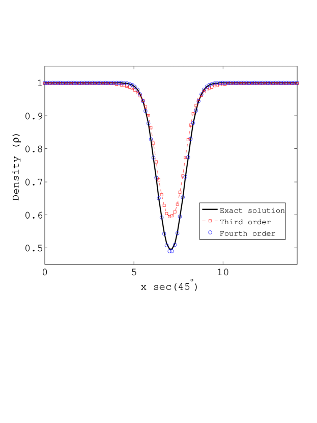
The 2D Euler vortex problem – We solve the 2D Euler vortex problem, described in the Section IV, for the present fourth order central scheme and the third order central scheme Kurganov and Levy (2000). Solutions are obtained at a resolution $96^{2}$ and density profiles, along the diagonal, are compared after $10$ periods $(t=100)$ which are shown in Figure 16. It is found from this nonlinear test that the present fourth order scheme has a significantly smaller numerical dissipation as compared to the third order scheme Kurganov and Levy (2000).

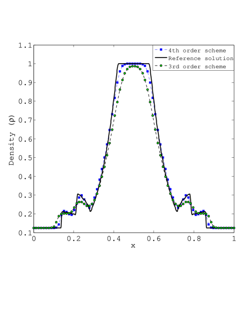
The 3D blast (explosion) test problem – The initial conditions for this test are same as described in the previous section. Here the solutions for both the schemes are obtained at time $t=0.1$ at a resolution $80^{3}$. Figure 17 shows the 1D profile of the density $(\rho)$ along the intersection of planes $y=0.5$ and $z=0.5$ for both the schemes and reference solution is obtained at a high resolution $720^{3}$ using the fourth order scheme.

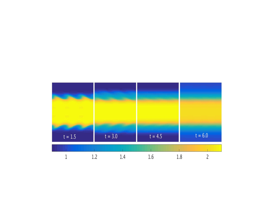
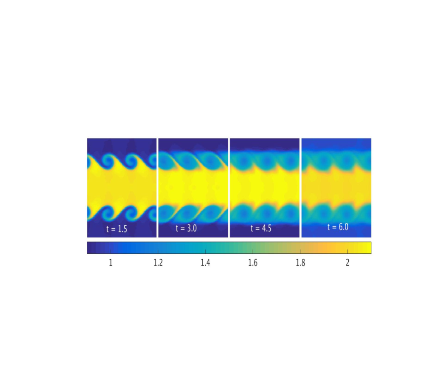
Kelvin-Helmholtz (KH) instability – The initial conditions for this test are same as described in the previous section, however, wavelength of the perturbation $\lambda$ is chosen to be $1/3$ and evolution of the KH instability is shown from time $t=1.5$ to $t=6.0$ as color-coded contour plots of the density in all the figures. Figures 18 and 19 show the evolution of the KH instability obtained from the third order CWENO scheme at a resolution $128^{2}$ and $256^{2}$, respectively. Note here that the intrinsic behaviour of the KH instability are captured at a resolution $256^{2}$, however, at $128^{2}$ resolution these features have vanished due to higher numerical dissipation of the third order CWENO scheme. In contrast, as is shown in figure 20 our fourth order CWENO scheme is able to capture these features even at $128^{2}$ resolution.

Computational cost – In TABLE 8 we compare the performance of the two schemes for 3D linear advection test and find that the third order scheme is on average $1.38$ times faster than present fourth order central scheme.

NG	Third order	Fourth order
$32^{3}$	1.0	1.36
$64^{3}$	1.0	1.41
$128^{3}$	1.0	1.41
$256^{3}$	1.0	1.40
$512^{3}$	1.0	1.32
Mean	1.0	1.38

Table 8: Performance test for the third and fourth order schemes where the run time is normalized with respect to the third order scheme.

Thus, we see that the implementation of the present fourth order central scheme involves an additional non-negligible but generally acceptable computational expense together with significantly reduced numerical dissipation when compared with the third order implementation Kurganov and Levy (2000).

VII Conclusion

A genuine multi-dimensional reconstruction for higher order schemes is complex and computationally more expensive than a dimension-by-dimension approach. Therefore, in this paper we have adopted a dimension-by-dimension CWENO approach to obtain a fourth order accurate central scheme. Different ways to employ a dimension-by-dimension CWENO approach have been discussed and the most efficient method has been applied to develop a fourth order CWENO scheme to solve multidimensional hyperbolic problems. The fourth order accuracy and the non-oscillatory property are confirmed in various multi-dimensional problems. The accuracy of the present dimension-by-dimension CWENO approach is found to be identical with truly multi-dimensional CWENO schemes. Moreover, the benefits of implementing the fourth order central scheme over third order central scheme have also been demonstrated by comparing the numerical dissipation and computational cost.

Fruitful discussions with J. Stone and P. Buchmüller are gratefully acknowledged and P.S.V. would also like to thank Tapan Chandra Adhyapak for useful suggestions.

Figure 1: (a) Sketch of a 3D grid cell and reconstructed area-averages $\overline{\bf U}_{i,j,k}^{\pm}$ at the grid cell interfaces $x_{i\pm 1/2}$ obtained from the 1D CWENO polynomial ${\bf R}_{i,j,k}(x)$ based on cell average $\overline{\bf U}_{i,j,k}$, (b) reconstructed three equi-distant edge-averages along the $y$-direction from the 1D CWENO polynomial ${\bf R}_{i,j,k}(y)$ based on area average $\overline{\bf U}_{i,j,k}^{+}$ at $x_{i+1/2}$, (c) reconstructed nine point values at $x_{i+1/2}$ from ${\bf R}_{i,j,k}(z)$ based on edge-averages in (b).

Figure 2: Density $(\rho)$ along the $x$-direction for the oblique shock tube problem at two resolutions ($200\times 50$) shown by ‘squares’ and ($600\times 150$) shown by ‘solid line’ at time $t=0.16632$. Here $n_{x}$ and $n_{y}$ are the number of grid points along the $x$ and $y$-directions, respectively.

Figure 3: Solution of the oblique Lax problem : 1D profile of the density $(\rho)$ at an angle $45^{\circ}$ with the $x$-axis obtained at a resolution $200^{2}$ (red squares) and $600^{2}$ (solid line) at time $(t=0.12)$.

Figure 4: Contour plot of the density ($\rho$) for the 2D blast wave problem at time $t=0.1$ at a resolution $100^{2}$.

Figure 5: Contour plot of the density ($\rho$) for the 2D blast wave problem at time $t=0.1$ at a resolution $200^{2}$.

Figure 6: Contour plot of the density ($\rho$) for the 2D Riemann problem at time $t=0.23$ at a resolution $200^{2}$.

Figure 7: Contour plot of the density ($\rho$) for the 2D Riemann problem at time $t=0.23$ at a resolution $400^{2}$.

Figure 8: Solution of the 3D Burgers’ equation at time $t=0.8$ : contour plot at the plane $z=0$ at a resolution $80^{3}$.

Figure 9: Solution of the 3D Burgers’ equation at time $t=0.8$ : contour plot at the plane $z=0$ at a resolution $400^{3}$.

Figure 10: Solution of the 3D blast wave problem at time $t=0.1$ : 1D profile of the density $(\rho)$ along the intersection of planes $y=0.5$ and $z=0.5$ where the solid squares stand for the fourth order accurate solution at a resolution $80^{3}$ and solid line is the reference solution.

Figure 11: Snap-shot of Kelvin-Helmholtz instability at time $t=0.7,1.4,2.1,2.8$ : color-coded contour plots of the density $(\rho)$ at a resolution $1024^{2}$.

Figure 12: Snap-shot of a 2D shock-bubble interaction at time $t=0.1$ : color-coded contour plots of the density $(\rho)$ at a resolution $400^{2}$.

Figure 13: Snap-shot of a 2D shock-bubble interaction at time $t=0.4$ : color-coded contour plots of the density $(\rho)$ at a resolution $400^{2}$.

Figure 14: Snap-shot of a 3D shock-bubble interaction at time $t=0.1$ : color-coded contour plots of the density $(\rho)$ at a resolution $400^{3}$ in the plane $z=0$.

Figure 15: Snap-shot of a 3D shock-bubble interaction at time $t=0.4$ : color-coded contour plots of the density $(\rho)$ at a resolution $400^{3}$ in the plane $z=0$.

Figure 16: Solution of the 2D vortex problem : 1D profile of the density $(\rho)$ at an angle $45^{\circ}$ with the $x$-axis obtained at a resolution $96^{2}$ after $10$ periods $(t=100)$ where squares represent the third order central scheme, circles stand for the present fourth order central scheme and the solid line ‘-’ is the exact solution.

Figure 17: Solution of the 3D blast wave problem at time $t=0.1$ at a resolution $80^{3}$: 1D profile of the density $(\rho)$ along the intersection of planes $y=0.5$ and $z=0.5$ where the solid squares stand for the fourth order accurate solution, circles depict the third order accurate solution and the solid line ‘-’ is the reference solution.

Figure 18: Evolution of Kelvin-Helmholtz instability at time $t=1.5,3.0,4.5,6.0$: color-coded contour plots of the density $(\rho)$ at a resolution $128^{2}$ using third order CWENO scheme.

Figure 19: Evolution of Kelvin-Helmholtz instability at time $t=1.5,3.0,4.5,6.0$ : color-coded contour plots of the density $(\rho)$ at a resolution $256^{2}$ using third order CWENO scheme.

Figure 20: Evolution of Kelvin-Helmholtz instability at time $t=1.5,3.0,4.5,6.0$: color-coded contour plots of the density $(\rho)$ at a resolution $128^{2}$ using fourth order CWENO scheme.

References

- Balbás and Tadmor (2006) Jorge Balbás and Eitan Tadmor. Nonoscillatory central schemes for one-and two-dimensional magnetohydrodynamics equations. ii: High-order semidiscrete schemes. SIAM Journal on Scientific Computing, 28(2):533–560, 2006.
- Bianco et al. (1999) Franca Bianco, Gabriella Puppo, and Giovanni Russo. High-order central schemes for hyperbolic systems of conservation laws. SIAM Journal on Scientific Computing, 21(1):294–322, 1999.
- Bryson and Levy (2003) Steve Bryson and Doron Levy. High-order semi-discrete central-upwind schemes for multi-dimensional hamilton–jacobi equations. Journal of Computational Physics, 189(1):63–87, 2003.
- Buchmüller and Helzel (2014) Pawel Buchmüller and Christiane Helzel. Improved accuracy of high-order weno finite volume methods on cartesian grids. Journal of Scientific Computing, 61(2):343–368, 2014.
- Cai et al. (2005) Li Cai, Jian-Hu Feng, and Wen-Xian Xie. A cweno-type central-upwind scheme for ideal mhd equations. Applied mathematics and computation, 168(1):600–612, 2005.
- Capdeville (2008) G Capdeville. A central weno scheme for solving hyperbolic conservation laws on non-uniform meshes. Journal of Computational Physics, 227(5):2977–3014, 2008.
- Capdeville (2011) G Capdeville. A high-order multi-dimensional hll-riemann solver for non-linear euler equations. Journal of Computational Physics, 230(8):2915–2951, 2011.
- Castro and Toro (2008) Cristóbal E Castro and Eleuterio F Toro. Solvers for the high-order riemann problem for hyperbolic balance laws. Journal of Computational Physics, 227(4):2481–2513, 2008.
- Cravero and Semplice (2016) Isabella Cravero and Matteo Semplice. On the accuracy of weno and cweno reconstructions of third order on nonuniform meshes. Journal of Scientific Computing, 67(3):1219–1246, 2016.
- Friedrichs and Lax (1971) Kurt O Friedrichs and Peter D Lax. Systems of conservation equations with a convex extension. Proceedings of the National Academy of Sciences, 68(8):1686–1688, 1971.
- Godunov (1959) Sergei Konstantinovich Godunov. A difference method for numerical calculation of discontinuous solutions of the equations of hydrodynamics. Matematicheskii Sbornik, 89(3):271–306, 1959.
- Holden et al. (1999) Helge Holden, Knut-Andreas Lie, and Nils Henrik Risebro. An unconditionally stable method for the euler equations. Journal of Computational Physics, 150(1):76–96, 1999.
- Hu and Shu (1999) Changqing Hu and Chi-Wang Shu. Weighted essentially non-oscillatory schemes on triangular meshes. Journal of Computational Physics, 150(1):97–127, 1999.
- Hu et al. (2010) XY Hu, Q Wang, and Nikolaus Andreas Adams. An adaptive central-upwind weighted essentially non-oscillatory scheme. Journal of Computational Physics, 229(23):8952–8965, 2010.
- Huang et al. (2014) Chieh-Sen Huang, Todd Arbogast, and Chen-Hui Hung. A re-averaged weno reconstruction and a third order cweno scheme for hyperbolic conservation laws. Journal of Computational Physics, 262:291–312, 2014.
- Ivan and Groth (2014) Lucian Ivan and Clinton PT Groth. High-order solution-adaptive central essentially non-oscillatory (ceno) method for viscous flows. Journal of Computational Physics, 257:830–862, 2014.
- Ivan et al. (2015) Lucian Ivan, Hans De Sterck, A Susanto, and Clinton PT Groth. High-order central eno finite-volume scheme for hyperbolic conservation laws on three-dimensional cubed-sphere grids. Journal of Computational Physics, 282:157–182, 2015.
- Ketcheson (2008) David I Ketcheson. Highly efficient strong stability-preserving runge–kutta methods with low-storage implementations. SIAM Journal on Scientific Computing, 30(4):2113–2136, 2008.
- Kissmann and Grauer (2007) R Kissmann and Rainer Grauer. A low dissipation essentially non-oscillatory central scheme. Computer physics communications, 176(8):522–530, 2007.
- Kleimann et al. (2004) Jens Kleimann, Andreas Kopp, Horst Fichtner, Rainer Grauer, and Kai Germaschewski. Three-dimensional mhd high-resolution computations with cweno employing adaptive mesh refinement. Computer Physics Communications, 158(1):47–56, 2004.
- Kurganov and Levy (2000) Alexander Kurganov and Doron Levy. A third-order semidiscrete central scheme for conservation laws and convection-diffusion equations. SIAM Journal on Scientific Computing, 22(4):1461–1488, 2000.
- Kurganov and Levy (2002) Alexander Kurganov and Doron Levy. Central-upwind schemes for the saint-venant system. ESAIM: Mathematical Modelling and Numerical Analysis, 36(3):397–425, 2002.
- Kurganov and Petrova (2001) Alexander Kurganov and Guergana Petrova. A third-order semi-discrete genuinely multidimensional central scheme for hyperbolic conservation laws and related problems. Numerische Mathematik, 88(4):683–729, 2001.
- Kurganov and Tadmor (2000) Alexander Kurganov and Eitan Tadmor. New high-resolution central schemes for nonlinear conservation laws and convection–diffusion equations. Journal of Computational Physics, 160(1):241–282, 2000.
- Kurganov and Tadmor (2002) Alexander Kurganov and Eitan Tadmor. Solution of two-dimensional riemann problems for gas dynamics without riemann problem solvers. Numerical Methods for Partial Differential Equations, 18(5):584–608, 2002.
- Kurganov et al. (2001) Alexander Kurganov, Sebastian Noelle, and Guergana Petrova. Semidiscrete central-upwind schemes for hyperbolic conservation laws and hamilton–jacobi equations. SIAM Journal on Scientific Computing, 23(3):707–740, 2001.
- Lahooti and Pishevar (2012) Mohsen Lahooti and Ahmadreza Pishevar. A new fourth order central weno method for 3d hyperbolic conservation laws. Applied Mathematics and Computation, 218(20):10258–10270, 2012.
- Langseth and LeVeque (2000) Jan Olav Langseth and Randall J LeVeque. A wave propagation method for three-dimensional hyperbolic conservation laws. Journal of Computational Physics, 165(1):126–166, 2000.
- (29) D Levy. A third-order 2d central scheme for conservation laws. Systém hyperboliques: Nouveaux schémas et nouvelles applications, 1:489–504.
- Levy et al. (1999) Doron Levy, Gabriella Puppo, and Giovanni Russo. Central weno schemes for hyperbolic systems of conservation laws. ESAIM: Mathematical Modelling and Numerical Analysis, 33(3):547–571, 1999.
- Levy et al. (2000a) Doron Levy, Gabriella Puppo, and Giovanni Russo. A third order central weno scheme for 2d conservation laws. Applied Numerical Mathematics, 33(1-4):415–421, 2000a.
- Levy et al. (2000b) Doron Levy, Gabriella Puppo, and Giovanni Russo. Compact central weno schemes for multidimensional conservation laws. SIAM Journal on Scientific Computing, 22(2):656–672, 2000b.
- Levy et al. (2000c) Doron Levy, Gabriella Puppo, and Giovanni Russo. On the behavior of the total variation in cweno methods for conservation laws. Applied Numerical Mathematics, 33(1-4):407–414, 2000c.
- Levy et al. (2002) Doron Levy, Gabriella Puppo, and Giovanni Russo. A fourth-order central weno scheme for multidimensional hyperbolic systems of conservation laws. SIAM Journal on scientific computing, 24(2):480–506, 2002.
- McCorquodale and Colella (2011) Peter McCorquodale and Phillip Colella. A high-order finite-volume method for conservation laws on locally refined grids. Communications in Applied Mathematics and Computational Science, 6(1):1–25, 2011.
- Nessyahu and Tadmor (1990) Haim Nessyahu and Eitan Tadmor. Non-oscillatory central differencing for hyperbolic conservation laws. Journal of computational physics, 87(2):408–463, 1990.
- Núñez-De La Rosa and Munz (2016) Jonatan Núñez-De La Rosa and Claus-Dieter Munz. xtroem-fv: a new code for computational astrophysics based on very high order finite-volume methods–i. magnetohydrodynamics. Monthly Notices of the Royal Astronomical Society, 455(4):3458–3479, 2016.
- Price (2008) Daniel J Price. Modelling discontinuities and kelvin–helmholtz instabilities in sph. Journal of Computational Physics, 227(24):10040–10057, 2008.
- Qiu and Shu (2002) Jianxian Qiu and Chi-Wang Shu. On the construction, comparison, and local characteristic decomposition for high-order central weno schemes. Journal of Computational Physics, 183(1):187–209, 2002.
- Schulz-Rinne et al. (1993) Carsten W Schulz-Rinne, James P Collins, and Harland M Glaz. Numerical solution of the riemann problem for two-dimensional gas dynamics. SIAM Journal on Scientific Computing, 14(6):1394–1414, 1993.
- Semplice et al. (2016) Matteo Semplice, Armando Coco, and Giovanni Russo. Adaptive mesh refinement for hyperbolic systems based on third-order compact weno reconstruction. Journal of Scientific Computing, 66(2):692–724, 2016.
- Shi et al. (2002) Jing Shi, Changqing Hu, and Chi-Wang Shu. A technique of treating negative weights in weno schemes. Journal of Computational Physics, 175(1):108–127, 2002.
- Shu (1998) Chi-Wang Shu. Essentially non-oscillatory and weighted essentially non-oscillatory schemes for hyperbolic conservation laws. In Advanced numerical approximation of nonlinear hyperbolic equations, pages 325–432. Springer, 1998.
- Shu (2009) Chi-Wang Shu. High order weighted essentially nonoscillatory schemes for convection dominated problems. SIAM review, 51(1):82–126, 2009.
- Sod (1978) Gary A Sod. A survey of several finite difference methods for systems of nonlinear hyperbolic conservation laws. Journal of computational physics, 27(1):1–31, 1978.
- Titarev and Toro (2004) Vladimir A Titarev and Eleuterio F Toro. Finite-volume weno schemes for three-dimensional conservation laws. Journal of Computational Physics, 201(1):238–260, 2004.
- Tokareva and Toro (2010) SA Tokareva and Eleuterio F Toro. Hllc-type riemann solver for the baer–nunziato equations of compressible two-phase flow. Journal of Computational Physics, 229(10):3573–3604, 2010.
- Toro (2013) Eleuterio F Toro. Riemann solvers and numerical methods for fluid dynamics: a practical introduction. Springer Science & Business Media, 2013.
- Williamson (1980) JH Williamson. Low-storage runge-kutta schemes. Journal of Computational Physics, 35(1):48–56, 1980.