Characteristics of He ii Proximity Profiles

Abstract

The proximity profile in the spectra of $z\approx 3$ quasars, where fluxes extend blueward of the He ii Ly $\alpha$ wavelength $304(1+z)$ Å, is one of the most important spectral features in the study of the intergalactic medium. Based on the HST spectra of 24 He II quasars, we find that the majority of them display a proximity profile, corresponding to an ionization radius as large as 20 Mpc in the source’s rest frame. In comparison with those in the H I spectra of the quasars at $z\approx 6$, the He II proximity effect is more prominent and is observed over a considerably longer period of reionization. The He II proximity zone sizes decrease at higher redshifts, particularly at $z>3.3$. This trend is similar to that for H I, signaling an onset of He II reionization at $z\gtrsim 4$.

For quasar SDSS1253+6817 ($z=3.48$), the He ii absorption trough displays a gradual decline and serves as a good case for modeling the He II reionization. To model such a broad profile requires a quasar radiation field whose energy distribution between 4 and 1 Rydberg is considerably harder than normally assumed. The UV continuum of this quasar is indeed exceptionally steep, and the He II ionization level in the quasar vicinity is higher than the average level in the intergalactic medium. These results are evidence that a very hard EUV continuum from this quasar produces a large ionized zone around it.

Distinct exceptions are the two brightest He II quasars at $z\approx 2.8$, for which no significant proximity profile is present, probably implying that they are very young.

1 INTRODUCTION

The epoch at redshift $\approx 3$ marks the peak of quasar formation (Richards et al., 2006) as well as the reionization of the intergalactic helium (Meiksin, 2009, M09 hereafter). As the reionization of singly ionized helium requires high-energy photons above 4 Rydberg, the hard UV background radiation field in the vast intergalactic space, commonly referred to as “metagalactic”, at $z\approx 3$ is believed to be photons originating from quasars instead of hot stars (Haardt & Madau, 1996; Meiksin, 2005). Because helium is difficult to ionize and readily recombines, its opacity at this redshift range is considerably higher than that of hydrogen.

Most of our knowledge of the intergalactic helium at these high redshifts is based upon a few bright quasars with clear lines of sight: QSO0302$-$003 (Jakobsen et al., 1994; Hogan, Anderson & Rugers, 1997; Heap et al., 2000), HS1700+6416 (Davidsen, Kriss & Zheng, 1996; Fechner et al., 2006) and HE2347$-$4342 (Kriss et al., 2001; Smette et al., 2002; Shull et al., 2004; Zheng et al., 2004; Shull et al., 2010). Thanks to the Sloan Digital Sky Survey (SDSS, York et al., 2000) and Galaxy Evolution Explorer (Martin et al., 2005), the number of known quasars with unobscured sightlines to their He II Ly $\alpha$ wavelengths has increased dramatically from only three in mid-1990s to more than 50 (Syphers et al., 2009a; Syphers et al., 2009b; Worseck et al., 2011). Of these quasars the highest redshift is 3.93 (Syphers et al., 2009b). The Cosmic Origins Spectrograph (COS, Green et al., 2012) instrument aboard the HST has greatly enhanced our ability to probe multiple lines of sight and investigate the He II absorption features at higher signal-to-noise (S/N) ratios. In the five years since the COS installation, more than two dozen quasars have been confirmed with the He II Ly $\alpha$ features.

The ensemble of spectra of these quasars is now sufficiently large that we can begin to overcome the cosmic variance and investigate the reionization process over a significant range of redshift. It is now well established that the Gunn-Peterson effect (Gunn & Peterson, 1965) in quasar spectra becomes significant only at $z\gtrsim 2.7$ for He II (Davidsen, Kriss & Zheng, 1996; Reimers et al., 1997; Anderson et al., 1999) and at $z\gtrsim 5.5$ for H I (Becker et al., 2001; Fan, Carilli & Keating, 2006), signaling the end of the respective reionization epochs. The intergalactic-medium (IGM) reionization process is lengthy, and little is known about the IGM evolution at much higher redshifts, i.e., $z\gtrsim 3.5$ for helium, $z\gtrsim 7$ for hydrogen.

The ionization properties of the IGM change significantly near luminous quasars, whose radiation enhances the ionization level in their vicinity. This “proximity effect” was first found in quasars at $z\approx 3$ where the number of H I Ly $\alpha$ forest lines in their optical spectra declines in the quasar vicinity (Murdoch et al., 1986; Carswell et al., 1987; Tytler, 1987b). At a high IGM opacity, the proximity effect results in an expected residual flux blueward of the He II Ly $\alpha$ wavelength (Zheng & Davidsen, 1995; Giroux, Fardal & Shull, 1995; Madau & Rees, 2000). Such an absorption profile has been observed in the H I spectra of most quasars at $z>5.7$ (White et al., 2003; Carilli et al., 2010). For helium, the presence of proximity profiles was ambiguous, as there were only a handful of known He II quasars, and some of them do not display a proximity profile.

The He II Ly $\alpha$ absorption troughs may be complex (Madau & Rees, 2000), as their shapes are affected by several factors: a proximity profile blueward of the He II Ly $\alpha$ wavelength, a damped absorption profile that extends to the wavelengths redward of it, and possibly another damped absorption profile from an associated absorber. In this paper, we report our analysis of the proximity effect using a large sample of quasars with confirmed He II Ly $\alpha$ features. The distances quoted in this paper are proper distances in the quasar’s rest frame, calculated using the codes of Hogg (1999), with the standard cosmological parameter values: $\Omega_{M}=0.3$, $\Omega_{\Lambda}=0.7$ and $h=H_{0}/100\,{\rm km\,s^{-1}\,Mpc^{-1}}=0.70$.

2 OBSERVATIONS AND ANALYSES

We investigate the HST spectra of 24 quasars in which the He II Ly $\alpha$ absorption feature is present at the anticipated wavelength and is not severely contaminated by geocoronal emission. Our database consists of three parts: (1) COS spectra of four quasars at $z>3.4$ from our program (GO 12249: PI Zheng), see Table 1; (2) archival COS spectra of seven quasars (GO 11742, 13013: PI Worseck); and (3) published spectra of 13 quasars, taken with COS and STIS. Six other quasars are excluded because their He II break is contaminated by geocoronal Ly $\alpha$ or O I $\lambda 1302$ emission. Table 2 lists the eleven sources in parts 1 and 2; and Table 3 lists the 13 sources in part 3.

Optical spectra of these quasars are useful as they provide information of the H I absorption counterparts. We retrieved 15 SDSS spectra of the He II quasars, the VLT/UVES spectra of quasars PKS1935$-$692 and HE2347-4342, and the Keck/HIRES spectra of QSO0302$-$003 and HS1700+6416. In total, we have the optical spectra of 17 quasars, among which four are at high resolution.

2.1 COS Spectra of Four Quasars

We carried out HST/COS spectroscopy of four quasars: SDSS1253+6817, SDSS1319+5202, SDSS1711+6052, SDSS2346$-$0016 (GO program 12249). They were selected as a bright sample (the UV continuum level at $\gtrsim 5\times 10^{-17}$ ${\rm erg\,s}^{-1}\,{\rm cm}^{-2}\,{\rm\AA}^{-1}$) at $z>3.4$ with confirmed He II Ly $\alpha$ absorption breaks with the ACS prism data (Zheng et al., 2008; Syphers et al., 2009a; Syphers et al., 2009b). The new COS data provide considerably higher S/N ratios and spectral resolution. The HST/COS observations of these four quasars were performed between 2010 November and 2011 December. The G140L spectra cover a wavelength range of approximately 1100-2150 Å with a pixel scale of 0.08 Å and resolution $R\approx 2000$. The source fluxes were extracted using a small slit width of 25 pixels, which is considerably smaller than the default size of 57 pixels (0${}^{\prime\prime}\!.$59, Syphers et al., 2012; Syphers & Shull, 2013). To determine the level of geocoronal-line contamination and scattered light, we reduced portions of the orbital night separately and compared with the full set. Only in one case (SDSS2346$-$0016) the airglow is significant even during the orbital night (Feldman et al., 1992), and the dataset taken in 2011 December has to be excluded.

The spectrum of SDSS1319+5202 reveals a Lyman-limit system (LLS) at $z\approx 0.7$ ($\sim 1550$ Å in the observed frame), and the source flux below 1550 Å is considerably suppressed. Based on low-resolution prism data ($R\simeq 105$ at 1460 Å), we suggested an associated damped absorption system whose effect extends redward of the He II Ly $\alpha$ wavelength (Zheng et al., 2008). With the improved wavelength accuracy of our higher-resolution COS spectrum, the absorption profile is confirmed to straddle the He II Ly $\alpha$ wavelength and cannot be explained by a simple proximity profile. The COS spectra of these four quasars are shown in Figure 1.

To study the absorption profiles, it is essential to accurately determine the quasar systemic redshifts. We retrieved the optical spectra of these quasars from the SDSS and used the IRAF task specfit (Kriss, 1994) to fit both the optical and UV spectra with multiple components. For the COS spectra, a power-law continuum, and a He II Ly $\alpha$ emission line were used to fit the data in wavelength redward of the He II Ly $\alpha$ break. For the optical spectra, we used a power-law continuum, multiple emission lines, including Ly $\alpha$ (narrow + broad), N V, O I, Si IV, C IV, He II (Vanden Berk et al., 2001), and a set of absorption templates that simulate the accumulated IGM absorption and the proximity profiles. The systemic redshifts were verified using the O I $\lambda 1304.22$ emission line as low-ionization lines are believed to be less affected by the local motion of broad-line regions. For our sample, the redshifts are generally consistent with those in the SDSS Data Release Seven Quasars Catalog (DR7, Schneider et al., 2010), except for SDSS2346$-$0016. We obtained a spectrum of SDSS2346$-$0016 using the TripleSpec instrument (Wilson et al., 2004) on the ARC (the Astrophysical Research Consortium) 3.5-m telescope. The observations were made on 2011 November 10 and 16, under an ambient temperature of 1-3 C, and the total integration time was 10 hours. As shown in Figure 2, the [O III] $\lambda$5007 emission is not visible. The Mg II and H$\beta$ emission lines, while unusually weak, yield a redshift consistent with the O I line. The COS spectra are of sufficient spectral resolution to confirm that that our measurements of the proximity profile are not affected noticeably by the small difference in quasar redshifts.

2.2 Archival COS Spectra of Seven Quasars

We retrieved the archival COS/G140L spectra of 15 other quasars (GO 11742 and 13013) via the Mikulski Archive for Space Telescopes and processed with the standard pipeline calcos (Hodge, 2011, v2.19). The difference between the pipeline extraction and our narrow-window extraction (see §2.1) is mainly in the residual flux level at wavelengths far away from the quasar, but this difference has no effect to our study. For QSO0233$-$0149, the geocoronal O I $\lambda 1302$ line is close to the He II Ly $\alpha$ wavelength, therefore we used the orbital-night portion of the data. We also used the night portion of the QSO0916+2405 data as geocoronal O I $\lambda 1356$ emission is near its He II proximity profile. Four of these quasars were excluded because of severe contamination by geocoronal emission. Four more were excluded as the flux breaks in their spectra are observed at wavelengths considerably longer than that for He II Ly $\alpha$. Most likely, these are attributed to partial He II LLSs along the lines of sight. The details of the seven archival spectra used are listed in the lower parts of Tables 1 and 2, below the details for our prime COS spectra listed at the top of the tables. Figure 3 plots the spectra of seven quasars that we include in our sample, with contaminating lines flagged with the Earth symbols.

2.3 Archival Data in the Literature

A number of the COS spectra of He II quasars have been published (Shull et al., 2010; Syphers et al., 2012; Syphers & Shull, 2013), most of which were observed with the G140L grating. We estimated the proximity sizes in the literature. For most of them, their systemic redshifts are from the SDSS catalog. The references for their redshifts are listed in Tables 3 and 4. One STIS spectrum of quasar PKS1935$-$692 is used.

2.4 Measurement of Proximity Zone Size

The study of He II proximity profiles is more challenging than that of H I at $z\approx 6$ as they are more complex. We measured a proximity zone from the He II Ly $\alpha$ wavelength to a point where the flux drops to below propagated errors as calculated in a bin of approximately 1.5 Å. We used these nominal bin sizes and combined the redshift errors to estimate the uncertainties in zone sizes. A difference of 1.5 Å corresponds to a redshift difference of 0.005 for He II Ly $\alpha$. This definition of proximity zones is based on an assumption of zero continuum flux beyond a proximity zone, as implied by the high He II opacity at $z\gtrsim 2.8$ (Shull et al., 2010; Syphers et al., 2011a).

An exception is the quasar HS1700+6416 ($z=2.751$), where the continuum flux level blueward of the He II Ly $\alpha$ wavelength is known to be nonzero. In Figure 8 of Syphers & Shull (2013), the He II Ly $\alpha$ absorption region is plotted along with a Keck/HIRES spectrum. We estimated the flux level in two regions where no strong H I absorption is present: $2.652<z<2.653$ and $2.6545<z<2.655$. The average He II Ly $\alpha$ opacity there was estimated as $\tau=0.95$. Extrapolating this value to $z=2.73$ using a theoretical scaling relation $\tau_{eff}\propto(1+z)^{3.5}$ (Fardal, Giroux & Shull, 1998), the normalized flux level there should be 0.36 ($\tau=1.03$). This is approximately the flux level around $z\simeq 2.728$ and 2.739, where no strong H I absorption features are present, and a potential flux excess near these two redshifts is marginal at best. It is likely that the proximity zone in HS1700+6416 ends at the absorption feature of $z\simeq 2.744$. A generous estimate would mark the zone down to $z\simeq 2.73$, where there is no significant H I absorption line. We therefore list the zone size as $4\pm 4$ Mpc in Table 3, to reflect the two possible values of 2 and 6 Mpc and other uncertainties.

All broad proximity profiles are embedded with strong absorption features. At a relatively high flux, these discrete absorption lines can be easily identified. However, at a low-flux end, they may cut off the residual flux and cause an underestimate of the proximity zone size. When an optical spectrum is available, we checked whether a strong H I absorption line is present near the wavelength that corresponds to the He II proximity zone’s endpoint. In six cases in Tables 2 and 3, no such a H I absorber is identified within 6 Å of the endpoint’s wavelength in optical spectra ($dz/(1+z)=0.001$). In the other 11 cases such H I absorption features are found near the proximity-zone endpoint, and for the other seven quasars no optical spectra are available. Therefore the possibility is real that their proximity zones may be underestimated. In these 18 cases we increased the measurement errors by adding a term of 3 Mpc ($dz/(1+z)=0.0035$ at $z=3.5$), approximately the nominal width of a strong absorption feature in G140L spectra. The quasar HE2347$-$4342 does not show a proximity zone, and there is no absorption feature in the UVES spectrum near the systemic redshift that can account for a potential He II LLS.

2.5 Correlation with Redshift and Luminosity

Given the sample size, it would be informative to study the evolution of He II proximity zones with redshift and luminosity, which has been reported for H I at $z\approx 6$ (§3.8). We plot the distribution of proximity-zone sizes over redshift and luminosity, respectively, in Figures 5 and 6. The redshift scales in the top and bottom panels of Figure 5 are set to reflect the same ratio of cosmic time. Our results demonstrate that the proximity effect is common among He II quasars, and their proximity-zone sizes can be considerably larger than those in the H I quasars at $z\approx 6$. The most significant trend seems to be at $z>3.3$, where the zone size decreases towards higher redshift. This trend may be understood in terms of an increasing He II fraction and signals the onset of the intergalactic He II reionization.

The two most luminous quasars, HS1700+6416 and HE2347$-$4342, are located at lower left in the top panel of Figure 6 and clearly disconnected from the rest of the sample. Recently a bright quasar at $z=6.3$ was discovered (Wu et al., 2015): with a similar luminosity and a moderate zone size, this quasar is also at odds with the model prediction that luminous quasars display a larger proximity zone.

We ran statistical tests to check potential correlations. The tool is the IRAF astronomical survival analysis package, which allows upper or lower limits as inputs (Isobe, Feigelson & Nelson, 1986). A moderate anti-correlation between zone sizes and quasar redshifts is confirmed: the Spearman correlation coefficient $\rho=-0.55$, rejecting a no-correlation hypothesis at 99% level. Proximity-zone sizes do not appear to be correlated with quasar luminosities: the Spearman correlation coefficient between them is $0.09$, suggesting a 65% probability for no correlation. Even without the two data points at the high-luminosity end, the correlation is still poor.

3 DISCUSSION

3.1 Uncertainties in Zone Size

A major source of uncertainties in our measurements of proximity zones is the systemic redshifts of quasars. The SDSS quasars have redshift uncertainties on the order of $dz/(1+z)\simeq 0.002$ (Hewett & Wild, 2010), which are derived mainly at $z<0.8$ when narrow emission lines are present. We verified the redshifts of SDSS quasars in our sample with O I $\lambda 1304$ emission in the optical spectra. O I $\lambda 1304$ emission is a weak feature and consists of multiple components, which carry a statistically weighted average of 1303.49 Å (Morton, 1991; Shull et al., 2010). Furthermore, O I $\lambda 1304$ emission may be blended with Si II $\lambda 1305.42$ (Vanden Berk et al., 2001). Assuming a solar abundance, the weighted average for O I+Si II is 1304.22 Å. We adopted this value with an uncertainty of 1 Å, which is comparable to the statistical errors of 5 Å (in the observer’s frame) in our fitting to the SDSS spectra. Combining these terms and converting into the observer’s frame for He II Ly $\alpha$, we estimated uncertainties of approximately 2 Å in the UV spectra of our sample. This term corresponds to $dz/(1+z)=0.0015$, 450 ${\rm km\,s}^{-1}$ in velocity dispersion, and 1.2 Mpc in proper distance at $z=3.5$. We verified the redshifts of SDSS quasars using fits to O I $\lambda 1304$ emission when possible. In a number of cases, O I $\lambda 1304$ emission is too weak to be useful in redshift estimates, we then used the redshift values from DR7. For the non-SDSS quasars in Tables 2 and 3, we assumed a redshift error of $\sim 800$ ${\rm km\,s}^{-1}$ in velocity space, unless quoted explicitly.

Another source of uncertainties in our estimates of the proximity-zone sizes arises from their ending points in the low-flux regions. Our data are mainly moderate-resolution spectra with limited S/N levels. For the COS G140L data, this nominal uncertainty is 1.5 Å, which corresponds to approximately 0.9 Mpc in proper distance at $z=3.5$ and 1.1 Mpc at $z=3.2$. As discussed in §2.4, the frequent occurrence of strong absorption features (H I column density $\approx 10^{14}$ $\rm cm^{-2}$) adds a term of uncertainty in many cases.

Other rare effects, such as an infalling absorber could affect the redshifts, but are unlikely to be thick enough to account for the lack of a proximity effect (Shull et al., 2010).

3.2 Effect of Intervening Hydrogen Lyman Limit Systems

Quasar spectra display the signature of numerous IGM components, and density fluctuations have a significant impact on the He II ionization process. LLSs of column density $\gtrsim 10^{17}$ $\rm cm^{-2}$, both in H I and low redshift and He II at high, produce random flux cutoffs. At $z\simeq 0.5$, a H I LLS may mimic a He II absorption edge. The probability of encountering such a system per unit redshift is $dn/dz=0.28(1+z)^{1.19}$ (Ribaudo, Lehner & Howk, 2011), which yields a rate that is consistent with other results (Storrie-Lombardi et al., 1994; Stengler-Larrea et al., 1995). Over a wavelength range of 15 Å ($\sim 10$ Mpc in proper distance) near He II Ly $\alpha$, there is less than 2% probability of intercepting a H I LLS of optical depth $\tau>1$. This value would be even smaller if we consider this effect only in the region near the proximity-zone’s endpoint.

3.3 Effect of intervening He II Lyman Limit Systems

For He II, the IGM components have considerably higher column densities and a filtering power. If the ratio of column densities $\eta=N_{HeII}/N_{HI}\gtrsim 100$, even a moderate H I absorber may become a potential He II LLS greatly reduce the number of He II-ionizing photons from the quasar, reducing both the growth of a He II ionization zone and the subsequent ionization rate.

A simple estimate (McQuinn et al., 2009) suggests that a system becomes opaque ($\tau>1$) to the ionizing photons at 4 Rydberg if its H I column density $N_{HI}>1.3\times 10^{16}(50/\eta)$ $\rm cm^{-2}$. Based on the high-resolution data at $z\simeq 2.8$ (Kriss et al., 2001; Zheng et al., 2004; Fechner et al., 2006), the mean value of $\eta$ is around 80, which is derived from a majority of weak components (column density $N_{HI}<3\times 10^{13}$ $\rm cm^{-2}$). At $3<z<3.2$, the mean $\eta$ value may be around 200 (Syphers & Shull, 2014). However, very high $\eta$ values are mostly associated weak lines and very difficult to confirm, particularly at $z>3$ when the He II opacity is high. Evidence suggests that strong components display lower $\eta$ values: Fechner et al. (2006) found $\eta\raisebox{-2.15277pt}{$\;\stackrel{{\scriptstyle<}}{{\sim}}\;$}15$ at $N_{HI}>3\times 10^{14}$ $\rm cm^{-2}$, which are supported by the data in another bright quasar ($\eta\raisebox{-2.15277pt}{$\;\stackrel{{\scriptstyle<}}{{\sim}}\;$}10$ at $N_{HI}>10^{15}$ $\rm cm^{-2}$, Zheng et al., 2004). Adopting a fiducial value of $\eta=15$, only the systems of H I column density $\gtrsim 4\times 10^{16}$ $\rm cm^{-2}$ may filter out the quasar He II-ionizing radiation. From Table 3 of Kim et al. (2013) the distribution can be expressed as $d^{2}n/(dN_{HI}dX)=10^{8.64}\ N_{HI}^{-1.54}$. The probability of encountering H I systems with $N_{HI}>4\times 10^{16}$ $\rm cm^{-2}$ within 1.5 Å to the endpoint of a proximity zone (see §2.4) is estimated as $\sim 0.02$.

Theoretical models, however, predict high $\eta$ around 100, based on our knowledge of the quasar’s EUV (extreme UV) continuum, and a re-analysis of the average $\eta$ values at $z\approx 2.5$ (McQuinn & Worseck, 2014) does not find evidence for the extremely low $\eta$ values noted in previous studies. This recent analysis is based on G140L data, while the previous studies used high-resolution FUSE data. To check the reality of low $\eta$ at $z\gtrsim 3$, we used the published results of QSO0302$-$003 at a higher redshift. Syphers & Shull (2014) used a high-resolution Keck spectrum and COS/G130M spectrum to derive $\eta$ values with a bin size of $dz=0.001$. In the range of $3.03<z<3.235$ there are 21 H I absorption lines at $N>10^{14}$ $\rm cm^{-2}$ (Kim et al., 2002). At $2.76<z<2.93$ and $3.25<z<3.267$ there are additional eight absorption lines with restframe equivalent widths greater than 0.3 Å. From Figures 10-13 of Syphers & Shull (2013) we estimated 29 $\eta$ values: twelve of them are lower limits and 17 are measurements. For the twelve lower limits, their mean value is $\eta=12$. For the 17 measured $\eta$ values, their mean value is 13.

If He II LLS are common, no broad proximity profiles should have been observed. We analyzed the SDSS spectra of our sample and identified 40 strong H I absorption features in the proximity zones: nearly all see a significant flux at their blueward wavelengths. If the $\eta$ values are around 100 for these absorbers, they should display a sharp flux cutoff. Furthermore, in the SDSS spectra of five quasars, no strong H I absorbers are found near the wavelengths that correspond to a proximity-zone endpoint (Tables 2 and 3). The upper limit to the H I column density would be approximately $10^{14}$ $\rm cm^{-2}$, assuming a minimum equivalent width of 0.3 Å in the restframe and a nominal velocity dispersion of 30 ${\rm km\,s}^{-1}$. If an endpoint of the proximity profiles in these quasars is attributed to an assumed He II LLS, the $\eta$ value may be 8000 or higher, which is not supported by observations. We therefore conclude that, while such a possibility cannot be ruled out, it is unlikely that proximity profiles are significantly altered by dense He II LLS.

3.4 He II Ionized Zone

The Strömgren radius is generally calculated from a balance of the ionizing photon rate with the total recombination rate (Strömgren, 1939; Cen & Haiman, 2000; Osterbrock & Ferland, 2006; Syphers, 2010). In a simple model, we assume that the IGM is homogeneous around a quasar, and the quasar radiation is isotropic. The total quasar ionizing luminosity in the restframe, in units of photon rate, is calculated as $\dot{N}_{\gamma}=4\pi D_{L}^{2}(1+z)^{-1}\int^{\infty}_{\nu_{0}}(f_{\nu}/h\nu)d\nu$ where $D_{L}$ is the bolometric luminosity distance, $f_{\nu}$ is the flux density in the observer’s frame and $\nu_{0}$ is the observed frequency corresponding to 4 Rydberg. The Strömgren radius is then:

$$R_{S}=\left(\frac{3\dot{N}_{\gamma}}{4\pi\alpha n_{e}n_{He_{III}}}\right)^{1/3}\approx 73\left(\frac{\dot{N}_{\gamma}/10^{57}s^{-1}}{\Delta^{2}}\right)^{1/3}\left(\frac{1+z}{4}\right)^{-2}\ \ \ {\rm Mpc}$$ (1)

where $\alpha$ is the Case-A recombination coefficient of He III ions, $n_{e}$ the electron density, and $\Delta$ the local baryon overdensity in units of the mean IGM density, and $R_{\rm S}$ the proper distance. The mean density of $1.85\times 10^{-5}$ $\rm cm^{-3}$ at $z=3.5$ is derived from its value at $z=0$ (Komatsu et al., 2011; Syphers, 2010).

The value given in Equation (1) is an upper limit; real ionized zones are considerably smaller for at least two reasons. First, this hypothetical limiting radius grows faster than the ionization front expands due to the decreasing IGM density as the Universe expands (Shapiro, 1986; Donahue & Shull, 1987). Secondly, for intergalactic helium, the recombination time scale is so long, $(\alpha n_{e})^{-1}\approx 1$ Gyr, that it exceeds the nominal quasar ages. As a result, the IGM around quasars would not reach a balance to form a Strömgren zone. If the gas is denser than average ($\Delta>1$) or clumpy, and if the quasar age is old, the recombination rate may become comparable to the ionization rate. A proximity zone does not mean that a Strömgren sphere has been established, in the sense of numbers of recombinations balancing numbers of ionizations. This calculation could just indicate that the gas within the sphere is over-ionized by the presence of the quasar radiation compared with that in the general IGM. The timing criterion for the ionization fraction to stay in ionization balance is only that the age be longer than (ionization rate)^-1 for highly ionized gas (M09).

Assuming an average IGM density, the opacity is estimated to be on the order of $2\times 10^{5}\ [(1+z)/6]^{3/2}$ for hydrogen and $4\times 10^{3}\ [(1+z)/4]^{3/2}$ for He II (Miralda-Escudé, 1998; Syphers, 2010). Syphers et al. (2011b) provide a more accurate formula that can be written for the chosen cosmological parameters:

$$\tau_{{\rm GP,HeII}}=3.49\times 10^{3}\ \Delta\ x_{\rm HeII}\left(\frac{Y_{P}}{0.2486}\right)\left(\frac{1+z}{4}\right)^{3/2}\\ \left[\frac{1.0209}{1+0.0209\cdot(4/(1+z))^{3}}\right]$$

where $x_{\rm HeII}$ is the He II fraction and $Y_{p}$ is the helium mass fraction.

In the vicinity of a luminous quasar, the ionizing radiation field is enhanced over any metagalactic ionizing background radiation, producing a cosmic “bubble” that may be observed in the quasar spectrum as a proximity effect. This effect should apply to H I (Murdoch et al., 1986; Bajtlik, Duncan & Ostriker, 1988) as well as He II (Zheng & Davidsen, 1995; Hogan, Anderson & Rugers, 1997) absorption. However, the overall He II optical depth could be as high as $\approx 4\times 10^{3}$ if the intergalactic helium is in a form of singly ionized state and remains poorly constrained at $z\gtrsim 3.3$.

In the wavelength region 1325-1340 Å ($z=3.362-3.411$) of the spectrum of SDSS1253+6817, the effective optical depth is $\tau_{HeII}=4.10^{+0.43}_{-0.33}$ at 95% confidence level. If we used a wider slit width as the calcos pipeline default, $\tau=5.10^{+1.02}_{-0.52}$ at 68% confidence level, or $\tau=5.10^{+\infty}_{-0.87}$ at 95% level. It is therefore possible that the flux extends beyond 12 Mpc from the quasar, suggesting that the metagalactic He II-ionizing radiation field is extremely weak but present, or the quasar has a He II-ionizing luminosity considerably stronger than the extrapolation from a nominal power law, or the ionization level has not yet recovered after an earlier episode of an enhanced quasar luminosity.

3.5 Effect of Quasar Age

The proximity profile is subject to the quasar age. A large zone size requires sufficient ionizing photons from the quasar, even after a long period, if the surrounding intergalactic helium was not fully ionized, and a large number of photons are needed to ionize it. For a young quasar, the proximity profile would display a sharp cutoff. Several factors affect the proximity profile: (1) the IGM density and its fluctuations; (2) the quasar luminosity; (3) the quasar age; and (4) the recombination process. For the case when the quasar age is considerably smaller then the recombination time scale, the total number of He II-ionizing photons over a lifetime $t_{Q}$ is equal to that of the ionized helium atoms in the quasar vicinity:

$$R_{\rm t_{Q}}=\left(\frac{3\dot{N}_{\gamma}t_{Q}}{4\pi n_{He}x_{\rm HeII}}\right)^{1/3}\approx 13\left(\frac{(\dot{N}_{\gamma}/10^{57}s^{-1})(t_{Q}/10^{7}yr)}{x_{\rm HeII}\ \Delta}\right)^{1/3}\left(\frac{1+z}{4}\right)^{-1}\ \ \ {\rm Mpc}.$$ (2)

We used the proximity profile in SDSS1253+6817 to model the evolution of intergalactic helium. While other cases of significant proximity effect exist, the profiles are often shelf-like, possibly due to the duty cycle of the quasar or the transverse proximity effect by other quasars (Syphers & Shull, 2014). The G140L spectrum, after a reddening correction of $E(B-V)=0.02$, $R_{V}=3.1$, and the extinction curve of Fitzpatrick (1999), displays a threefold increase in flux from 1950 to 1400 Å, which is steeper than that in QSO0302$-$003. Since no LLS break is obvious in this wavelength range, we fitted the dereddened continuum between 1400 and 1900 Å with a simple power law and a potential partial LLS between 2000 and 3000 Å. The best fit suggests $\beta=-2.09$ ($f_{\lambda}\propto\lambda^{\beta}$) and a LLS of $\tau=0.83$ at $\sim 2450$ Å. If no LLS is assumed, the best-fit power law has $\beta=-2.85$. Both fitting results suggest a similar continuum level of $(4.6\pm 0.5)\times 10^{-16}$ ${\rm erg\,s}^{-1}\,{\rm cm}^{-2}\,{\rm\AA}^{-1}$at the He II Lyman-limit wavelength of $1020$ Å. The estimated total photon rate at 4 Rydberg is $(5.9\pm 0.6)\times 10^{56}$ sec^-1. As shown in the next section, this hard continuum is not strong enough to produce the observed broad proximity profile if the intergalactic helium is not fully ionized.

3.6 Time Dependence of Ionization

The ionized zones represented by Equations (1) and (3) are extreme cases; the real ionization by a quasar is a gradual and slower process, which can be described by an analytical expression derived from a simplified differential equation (Cen & Haiman, 2000; Syphers & Shull, 2014) for a fixed IGM temperature. A more accurate evaluation of the ionization fraction requires simultaneously solving for the gas temperature and the ionization. We computed the time dependence of He II ionization around a quasar, as outlined in M09. Specifically, we solved the time-dependent spherically symmetric set of coupled ionization rate equations for uniformly distributed hydrogen and helium (Equations 41 and 46 of M09) on a radial grid, including the photoelectric attenuation by H I, He i and He II of the radiation from the quasar. We solved these equations simultaneously with the photoionization heating and cooling equations as described in M09 (sec.III.B) for a pure hydrogen/helium gas of cosmic abundances. This calculation used the atomic rates in M09, except for adopting the electron excitation and ionization cooling rate of H I from Scholz & Walters (1991). Our calculations assumed Case A recombination and included Compton cooling off the cosmic microwave background and adiabatic expansion losses in the gas. We considered a sequence of quasar activation redshifts corresponding to He III-region ages at $z=3.48$ of 10, 20, 30, 50, and 100 Myr. To match the observed proximity profile, the He II-ionizing continuum must be very strong: $L_{\nu}=6\times 10^{31}{\rm erg\ s^{-1}Hz^{-1}}$ at 228 Å in the restframe, which is approximately three times of the estimated level from observations. It would imply an EUV continuum that is even steeper than QSO0302$-$003 (Syphers & Shull, 2014). Lower-luminosity models, such as a He II-ionizing continuum extrapolated from the flux at He II Ly $\alpha$ wavelength with a nominal power-law index of $-1.7$ (Zheng et al., 1997; Telfer et al., 2002) were not able to match the size of the ionized region and the flux simultaneously. We emphasize that the measured absorption signal is co-temporaneous with the quasar observed. Since the characteristic time to reionize the gas and maintain ionization equilibrium is on the order of millions to tens of millions of years, depending on the distance from the quasar, the luminosity of the quasar that produced the proximity zone may have been larger than the observed value; we have few constraints on quasar variability on million year timescales.

We estimated the black-hole mass as $2.4\times 10^{9}$ M_⊙, using the C IV line width, the underlying continuum flux in the SDSS spectrum and the formula in Vestergaard & Peterson (2006). Following the work of Steinhardt & Elvis (2011), we derived the rest-frame luminosity near the Lyman limit as $2\times 10^{47}$ ${\rm erg\,s}^{-1}$, which is below the Eddington limit of $3\times 10^{47}$ ${\rm erg\,s}^{-1}$. A He II-ionizing metagalactic background was not assumed. In our simulations of the ionization zone, a hydrogen-ionizing and He i-ionizing metagalactic background was turned on at $z=7$. Figure 7 shows the He II ionization level, the IGM temperature and the normalized observed He II flux at different epochs after the quasar’s birth.

Shortly after the quasar’s birth, a sharp ionization front expands over time, as described by Equation (3). At each radius and each time interval, the temperature is computed from the energy equation and used to evaluate the atomic rates. Helium within the sphere is highly ionized, as the ionizing flux is strong and recombination is not effective. At later epochs, when the ionization front reaches large distances, ionization balance between the geometrically-diluted quasar ionization flux and recombinations produces a more gradual rise in the He II fraction with distance. As shown in Figure 7, a smooth decline of flux may be observed after $\approx 30$ Myr.

The high luminosity assumed in this simulation and that in Equation (3) probably represents an upper limit as high-energy photons from the quasar need to ionize a large volume of singly ionized helium. This requirement would be eased if a He II-ionizing background field existed prior to $z\approx 3.5$. As Equation (2) shows, the ionizing luminosity may be reduced by a factor of three to $6\times 10^{56}$ sec^-1 if the He II fraction $x_{\rm HeII}$ is 30%. In either case, the ionization front is likely moving nearly at the speed of light, as shown in Figure 7. White et al. (2003) studied the time-retardation effects on the observed proximity-zone size. Adapting their equations to He II, the speed-of-light corrections are important to the observed size until times large compared with $t_{c}\approx 100$ Myr for an assumed boosted quasar He II ionizing photon luminosity of $1.9\times 10^{57}\,{\rm sec}^{-1}$, where $t_{c}=(3\dot{N}_{\gamma}/4\pi n_{\rm HeIII}c^{3})^{1/2}$. The observed ionization zone sizes then increase slowly with time, as $t^{1/3}$. After an expansion time of 50 Myr, the ionization front in Figure 7 is restricted by the speed of light, but the ionization front velocity slows to 0.5c by 100 Myr. According to Equation (3), the age of the observed quasar producing the ionization zone after an expansion time of 50 Myr is $t_{Q}=12$ Myr, which provides a minimal age to the quasar.

If the IGM were highly clumped, the He II region would expand more slowly, as recombinations would slow it down. The high quasar luminosity used in Figure 7 is required to match both the position of the He III ionization front and the He II Ly $\alpha$ flux level behind the front assuming a homogeneous IGM. If instead the IGM opacity is dominated by line-blanketing by the Ly $\alpha$ forest, the quasar luminosity need not be so high to match the flux level while still matching the position of the He III front. This would, however, require a somewhat older quasar. The model in Figure 7 demonstrates the extreme assumptions that must be made for the quasar spectrum to match both the flux level and the position of the He III front assuming a homogeneous IGM. Line-blanketing by the He II Ly $\alpha$ forest is a more plausible explanation for the flux level (Madau & Meiksin, 1994).

3.7 Helium Proximity Effect in the Literature

In principle, a proximity profile should be present in every He II quasar spectrum, as a cosmic “bubble” would exist even without a metagalactic radiation field. At the beginning, ionizing photons do not travel very far, as the mean free path $(\sigma_{HeII}n_{HeII})^{-1}$ is less than 0.1 Mpc, where $\sigma_{HeII}=1.6\times 10^{-18}$ cm² is the photoionization cross section at 4 Rydberg and $n_{HeII}\simeq 2.5\times 10^{-6}$ cm^-3 the number density of singly ionized helium at $z=4$, is less than 0.1 Mpc. High-energy photons from the quasars, however, penetrate considerably deeper into the IGM, raising its temperature (Tittley & Meiksin, 2007; McQuinn et al., 2009). These ionized spheres expanded and eventually overlapped, gradually completing the reionization of intergalactic helium. While it is anticipated that luminous quasars exhibit a broader proximity profile (Equations (1) and (3)), it is not the case for the two brightest He II quasars at $z\approx 2.8$. The UV spectroscopic properties of HS1700+6416 ($z=2.751$, V=16.2) have been extensively studied (Davidsen, Kriss & Zheng, 1996; Fechner et al., 2006; Syphers & Shull, 2013). Its proximity profile is insignificant, extending at most 6 Mpc (see §2.4). The other well-known quasar, HE2347$-$4342 ($z=2.887$, V=16.1, Reimers et al., 1997; Kriss et al., 2001; Shull et al., 2004; Zheng et al., 2004) has no proximity effect observed. The redshifts from O I $\lambda$1304 and O III $\lambda$5007 agree (Reimers et al., 1997; Syphers et al., 2011a). There may be a strong infalling absorption system observed in the UV spectrum (Fechner et al., 2004; Shull et al., 2010). Shull et al. (2010) studied this infalling system and concluded that no satisfactory explanation exists for the absence of a proximity effect around this luminous quasar other than the possibility that it has only recently turned on (within the last Myr)

Hogan, Anderson & Rugers (1997) and Heap et al. (2000) discovered a He II proximity zone in the quasar QSO0302$-$003 at $z\approx 3.286$ (V=17.5). Blueward of the break, a shelf of residual flux corresponding to an opacity $\tau\approx 0.8$ extends out about 15 Å. The recent COS observations (Syphers & Shull, 2014) provide details in the proximity zone. The broad proximity profile, extending up to 15 Mpc, may be attributed to a line-of-sight effect from the quasar itself, or to a transverse effect by another quasar Q0301$-$00 ($z=3.232$) near the line of sight. In the latter case, the age of the ionization zone around Q0301$-$00 should be at least 34 Myr. It is interesting to note that the He II-ionizing continuum is considerably harder (power-law index $-0.8$) than previous work suggested: broad proximity profiles appear to be related to a hard quasar continuum. Similarly, in PKS1935$-$692 ($z\simeq 3.18$, Anderson et al., 1999), a proximity shelf of flux extends blueward of the He II break by at least 20 Å. This absorption feature displays a strong recovery void at 1246.5 Å, likely produced by the radiation of a foreground source.

3.8 Comparison with Hydrogen Proximity Effect

The reionization of intergalactic hydrogen ended by redshift $z\approx 6$, as characterized by a sharp increase in opacity at $z>5.7$ (Fan, Carilli & Keating, 2006). This trend is similar to what is observed for helium at $z\approx 3$, and it is instructive to compare these two major cosmic processes. The number of H I-ionizing photons of a quasar is considerably higher than that of He II-ionizing photons. On the other hand, the IGM at $z\approx 6$ is denser than that at $z\approx 3.5$. The recombination time scale of hydrogen is lower than helium. As a result of these factors, our estimate based on Equation (1) suggests that the proximity profile of intergalactic hydrogen at $z\approx 6$ is somewhat weaker than that for He II at $z\approx 3$.

Carilli et al. (2010) reported proximity profiles of hydrogen in the spectra of 27 quasars; their “near zones” (proximity) lie in the range of $\sim 5-10$ Mpc. They found a significant trend for a decrease in the near-zone size with increasing redshift, as evidence for the evolution of an increasing neutral fraction of intergalactic hydrogen toward higher redshifts. They also found that the near-zone sizes increase with the quasar UV luminosity, as expected for photoionization dominated by quasar radiation. We add eight more data points from recent literature. One quasar is at the highest known redshift $z\simeq 7.08$ (Mortlock et al., 2011) and another is luminous ($M=-29.3$, Wu et al., 2015). These two data points carry a significant weight in the correlation analysis. The paper of Venemans et al. (2013) does not list the near-zone sizes, and we made estimates from their Figure 4. A Spearman test over these 35 data points finds a correlation coefficient $\rho=-0.59$ between zone sizes and redshifts, rejecting a no-correlation hypothesis at 99.95% level. Another test between zone sizes and absolute magnitude finds $\rho=-0.47$, rejecting a no-correlation hypothesis at 99.4% level.

The luminous quasar J0100+2802 displays a proximity zone of 8 Mpc. While this is a significant size, it does not scale well to luminosity (see the lower panel of Figure 6). Its normalized zone size, $R_{norm}=R\ 10^{0.4(27+M_{1450})/3}$ at the restframe wavelength of 1450 Å, is 4 Mpc, below the average at the absolute magnitude $M_{1450}=-27$. This result is actually consistent with the two luminous He II quasars that they do not show a significant proximity profile. Maybe some other factors, such as the density and ionization level in the quasar’s vicinity or a young quasar age, play an important role.

4 CONCLUSION

We utilize a sample of 24 He II quasars to investigate the interplay between these quasars and the surrounding IGM. The ionization zone around He II quasars is often more prominent than that for H I at $z\approx 6$. The large redshift range for these quasars allows us to gain insight into the IGM reionization over a long epoch before intergalactic helium became fully ionized. The proximity-zone sizes decline significantly at $z>3.3$, and it is likely that helium reionization started well before $z=3.8$.

In the quasar SDSS1253+6817, the source flux extends considerably blueward of the He II Ly $\alpha$ wavelength, suggesting a quasar age of $\gtrsim 12$ Myr. The UV flux rises dramatically from 1950 to 1400 Å, suggesting an exceptionally hard EUV continuum. The $\eta$ value in the proximity zone is lower, consistent with such strong He II-ionizing radiation from the quasar that produces a broad proximity zone.

The two brightest quasars do not display a significant He II proximity profile. While this is at odds with model expectations, we notice that a luminous quasar does not display the largest H I proximity profile either. It is possible that these hyperluminous quasars are young, or they are surrounded by a dense IGM.

It should be stressed that the observed proximity-zone size is not a direct measurement of the quasar lifetime, as the structure of the zone is affected by many possible factors, including the IGM density fluctuations and quasar variability over IGM ionization timescales. A quasar with small proximity zone may be considerably younger compared with the light-travel time across its proximity zone allowing for retardation effects. Further understanding of the quasar lifetime awaits improved IGM simulations that take these factors into account.

APPENDIX A

ACS PRSIM SPECTRA

Approximately half of all the known He II quasars were discovered in three ACS prism surveys (GO 10907, 11215, 11982: PI Anderson; Syphers et al., 2009a; Syphers et al., 2009b). The ACS PR130L prism offers a low spectral resolution, $R\approx 170-380$ between 1360 and 1250 Å. While the potential merit of these prism spectra is limited, their sample size is significant. It is therefore interesting to explore the proximity profiles in the “other half” of the He II quasar sample. We estimated the proximity profiles in the published prism spectra of 15 quasars at $z<3.6$. The spectra of six other quasars at higher redshifts were not used because the spectral resolution degrades significantly redward of 1400 Å.

To understand the effect of spectral deconvolution, we simulated thousands of spectra with different proximity profiles ($0-25$ Å) at $z=3.5$ and a pixel scale of 0.1 Å, then convolved with a Gaussian kernel appropriate to the wavelength-dependent ACS resolution. The input spectra were of simple constant flux, with a proximity profile that starts at 1367 Å and declines linearly towards zero at the end of the proximity zone. The flux at shorter wavelengths of the proximity zone was set to zero. The noise level was set for an exposure time of 4500 sec, which is typical for these prism observations. As the S/N level in prism spectra is quite high ($>10$), our simulation results are not sensitive to noise. Each of these simulated spectra was smoothed to a resolution of the PR130L prism and then binned with small wavelength offsets. These offsets reflect the possibility that a spectrum may shift within a prism-data pixel and subsequently affect the deconvolution result. These simulated prism data were deconvolved using the IDL task MAX_LIKELIHOOD with a point-spread-function kernel of two pixels and then compared with the input data.

Our measurements of proximity zones in approximately 90% of the simulated spectra were within an error of one prism pixel ($\sim 4$ Å), and the others recovered within two pixels. A conservative estimate for the errors in prism data as 7 Å ($\simeq 5$ Mpc at $z=3.5$), which are considerably higher.

We compared the COS/G140L spectra of quasars SDSS1253+6817 and SDSS2346$-$0016 with their counterparts in the ACS/PR130L prism data. As shown in Figure 8, prism spectra display an extended wing at a level $<10\%$ of the unattenuated flux. This may be due to the extended wing of the instrumental line-spread function or potential misalignment of a few individual prism images. We measured the proximity zone to a flux level of 10% level. The proximity profiles in the prism data are consistent with that in the COS/G140L data: SDSS1253+6817 displays a broad profile and SDSS2346$-$0016 does not.

Most of the ACS prism data yielded no detection of proximity profiles ($\lesssim 5$ Mpc). In Table 4 we list three quasars whose proximity profiles in the ACS prism spectra are larger than 7 Å. They are at relatively high redshifts, and the data suggest that the decline of proximity-zone size may start at $z\simeq 3.5$.

APPENDIX B

PROXIMITY EFFECT in SDSS DATA

The study of the proximity effect has been based on high-resolution quasar spectra (Murdoch et al., 1986; Bajtlik, Duncan & Ostriker, 1988; Dall’Aglio, Wisotzki, & Worseck, 2008b), where the numbers of forest lines are compared in the quasar’s vicinity and at large distances. The effect of enhanced radiation in a quasar’s vicinity may be seen even at a low spectra resolution. Dall’Aglio, Wisotzki, & Worseck (2008a) used a flux transmission technique on the VLT/FORS2 spectra ($R\sim 800$) of 17 bright quasars at $2.7<z<4.1$ to measure the effective optical depth along the lines of sight and detect a proximity effect.

The effective optical depth accumulated from most IGM components is estimated as

$$\tau=0.0021(1+z)^{3.7}$$ (3)

(Meiksin, 2006; Kirkman et al., 2007; Becker et al., 2013). Approximately half of this term is from those at column density $N>10^{14}$ $\rm cm^{-2}$, most of which cases can be identified at the SDSS spectral resolution and S/N (§2.4). From a power-law distribution of $dn/dN_{HI}\propto N_{HI}^{-1.6}$ where $N$ is the column density and $n$ the number of individual absorbers (Tytler, 1987a; Janknecht et al., 2006), we estimated approximately six strong absorbers over a range of 10 Mpc ($\sim 66$ Å on the SDSS wavelength scale). These lines affect roughly 60% of the pixels in this bin, assuming that each line affects five SDSS spectral pixels. The fluxes in other pixels in this bin are believed to bear the signature of weak IGM components. Since these lines are unsaturated, their intensity is sensitive to the proximity effect. By measuring the flux decrements in these pixels, we tried to detect the signature of proximity zones.

We generated a set of absorption templates $\tau=0.0021(1+z)^{3.7}/(1+(R_{p}/r)^{2})$, where r is the distance to the quasar and $R_{p}$ the proximity size. The range of $R_{p}$ is 5$-$35 Mpc. The fitting task specfit allows such a “userabs” component in the form of opacity vs. wavelength. We ran specfit on SDSS spectra with the following components: an underlying power law, Gaussian emission components of Ly $\alpha$ (narrow + broad), N V, O I, Si IV, C IV, He II, and a set of absorption templates. The fitting windows consists of two parts at the following restframe wavelengths: (1) 1216$-$1680 Å, which cover the red wing of Ly $\alpha$ and five other emission lines (§2.1) and (2) a number of small windows between 1200 and 1216 Å, where no strong forest line is detected.

We ran tests on the SDSS spectra two quasars with different He II proximity zones. For SDSS1253+6817, our fitting results suggest a symmetrical Ly $\alpha$ profile, implying a strong proximity profile. The average opacity $\tau_{eff}=0.03\pm 0.03$ over a bin $20-80$ Å blueward of the Ly $\alpha$ wavelength. The calculation includes 22 pixels that are not in absorption windows. For SDSSJ1711+6052, the fitting result suggests that the blue Ly $\alpha$ wing is weaker than the red wing, as expected from IGM absorption. The average optical depth in a similar wavelength range is $\tau_{eff}=0.46\pm 0.33$. The S/N in the second quasar is $\simeq 7$ per pixel in the proximity zone, and the errors in our measurements are dominated by pixel-to-pixel variations. A higher average optical depth with noticeable pixel-to-pixel fluctuations is consistent with a significant structure in the forest lines and a weak proximity effect. These fitting results suggest that the signature of a broad proximity zone may be detected in SDSS spectra.

Table 1: Summary of Observations

Quasar	R.A.	Decl.	Observation	Exposure Time	Grating Central
	(J2000)			(sec)	Wavelength (Å)
Data of GO 12249
SDSS1253+6817	12 53 53.715	68 17 14.20	2011 May	14095	1105/1280
SDSS2346$-$0016	23 46 25.662	$-$00 16 00.47	2010 Nov., Dec.	20737	1105/1280
SDSS1711+6052	17 11 34.412	60 52 40.39	2011 Apr., Oct.	23950	1105
SDSS1319+5202	13 19 14.205	52 02 00.11	2011 May	26643	1105
Archival Data of GO 11742, 13013
SDSS1237+0126	12 37 48.993	01 26 06.90	2010 Jun.	6212	1105
QSO2149$-$0859	21 49 27.770	$-$08 59 03.61	2013 Apr.	7561	1105
SDSS0936+2927	09 36 43.511	29 27 13.60	2011 Jan.	4739	1105
QSO1630+0435	16 30 56.340	04 35 59.42	2013 Apr.	7908	1105
QSO2157+2330	21 57 43.630	23 30 37.34	2013 Jul.	8074	1105
QSO0233$-$0149	02 33 06.010	$-$01 49 50.58	2013 Aug.	2021	1105
QSO0916+2405	21 57 43.630	23 30 37.34	2013 Dec.	3075	1105

Table 2: Proximity Zone Measurement

Quasar	Redshift		Observed Continuum Flux $f_{\lambda 0}(304)$	Magnitude	Proximity Zone Size
	This work	SDSS	$10^{-17}$ ${\rm erg\,s}^{-1}\,{\rm cm}^{-2}\,{\rm\AA}^{-1}$	$M_{1450}$	Å	Mpc
Data of GO 12249
SDSS1253+6817	$3.476\pm 0.004$	3.4727	19	$-27.3$	20	12
SDSS2346$-$0016	$3.511\pm 0.003$	3.4895	19	$-28.0$	6	3.5
SDSS1711+6052	$3.823\pm 0.007$	3.8269	8	$-26.6$	5	2.5
SDSS1319+5202	$3.93\pm 0.01$	3.8991	2	$-28.2$	$10$	4.7
Archival Data of GO 11742, 13013
SDSS0936+2927	$2.9253\pm 0.004$	2.9239	15	$-27.4$	20	16
QSO2157+2330	3.142		15	$-27.7$	26	19
SDSS1237+0126	3.1448		15	$-26.8$	11	8
QSO2149$-$0859	3.259		6	$-26.9$	4	2.7
QSO0233$-$0149	3.314		11	$-27.2$	11	7.2
QSO0916+2405	3.440		18	$-27.0$	7	4
QSO1630+0435	3.788		23	$-28.3$	10	5.1

Table 3: He II Measurement Based on Published COS and STIS Data

Quasar	Redshift	Magnitude	Proximity Zone Size		Reference
		$M_{1450}$	(Å)	(Mpc)
HS1700+6416	$2.751\pm 0.003$	$-29.4$	4	3.7	Syphers & Shull (2013)
Q1216+1656	2.818	$-27.3$	15	13	Syphers et al. (2012)
HS1024+1849	2.8475	$-27.0$	21	18	Syphers et al. (2012)
4C57.27	2.858	$-27.1$	11	9	Syphers et al. (2012)
HE2347$-$4342	$2.885\pm 0.005$	$-29.3$	0	0	Shull et al. (2010)
SDSS1508+1654	3.1716	$-27.3$	18	12	Syphers et al. (2012)
PKS1935$-$692	3.185	$-28.3$	25	17	Anderson et al. (1999)
SDSS0856+1234	3.1948	$-27.0$	20	14	Syphers et al. (2012)
SDSS0955+432	3.2388	$-26.2$	18	12	Syphers et al. (2012)
QSO0302$-$003	3.2860	$-28.3$	17	11	Syphers & Shull (2014)
SDSS0915+4756	3.3369	$-27.9$	6	3.9	Syphers et al. (2012)
SDSS2345+1512	3.5880	$-26.6$	5	2.8	Syphers et al. (2012)
SDSS2257+0016	3.7721	$-27.2$	5	2.6	Syphers et al. (2012)

Table 4: He II Measurement Based on Published ACS Prism Data

Quasar	Redshift	Magnitude	Proximity Zone Size		Reference
		$M_{1450}$	(Å)	(Mpc)
SDSS1042+5129	3.3864	$-27.1$	26	17	Syphers et al. (2011b)
SDSS1007+4723	3.4084	$-26.2$	9	6	Syphers et al. (2009b)
SDSS1442+0920	3.5286	$-28.3$	13	8	Syphers et al. (2009b)

Figure Captions

HST/COS G140L spectra of four quasars. The data are binned by six pixels ($\approx 0.5$ Å, 0.85 resolution elements). The green dotted curves are the errors, and the red dashed lines mark the wavelengths of He II Ly $\alpha$. Vertical bars mark the wavelength of strong absorption lines identified from the SDSS spectrum counterparts, and arrows mark the edge of proximity zones.

Near-infrared spectrum of SDSS2346$-$0016, taken with the ARC 3.5-m telescope and TripleSpec instrument. Gaps in wavelengths are due to the removal of poor data in the bands of severe atmospheric absorption. The inset displays the wavelength region for redshifted Mg II emission. We used it to determine the systemic redshift of $z=3.511$.

HST/COS G140L spectra of seven other quasars in the HST archive, plotted in the quasar’s restframe. The data are binned by six pixels ($\approx 0.5$ Å). The green dotted curves are the errors, and the red dashed lines mark the wavelengths of He II Ly $\alpha$. The Earth symbols mark the wavelengths of the strong geocoronal lines around 1216 and 1302 Å, and a weak one at 1356 Å. Vertical bars mark the wavelength of the strong absorption lines identified from the SDSS spectrum counterparts, and arrows mark the edge of proximity zones.

Normalized spectra of quasar SDSS1253+6817. The lower panel is the He II Ly $\alpha$ region in the observer’s wavelength frame (COS/G140L), and the upper panel is the aligned H I counterparts (SDSS). The proper distance scale in the top label is appropriate for both panels. The green shaded region marks the wavelength range for the He II Ly $\alpha$ break, given the redshift uncertainty ($z=3.472-3.480$). The magenta arrow marks the wavelength for the ending point of the estimated proximity zone. The blue lines mark respective baselines and data errors. The red bars mark the strong absorption features identified in the SDSS spectrum.

Size of proximity zone vs. redshift. In the upper panel, red boxes are COS data, GO 12249; magenta boxes: archival data of GO 11742 and 13013; green boxes: COS data from literature; the cyan star: STIS data of PKS1935$-$692. The downward arrow is for $1\sigma$ limit with non-detection. The lower panel is for H I. Black crosses are from Table 1 of Carilli et al. (2010); green circles: Venemans et al. (2013, 2015); and red triangles: Mortlock et al. (2011); Wu et al. (2015). The redshift ranges in the two panels are scaled to represent the same ratio (1.0:0.65) of cosmic ages from the Big Bang.

Size of proximity zone vs. absolute magnitude. The symbols are the same as Figure 5. Yellow curves represent model predictions of $R_{s}\propto L^{1/3}$. The very luminous quasars ($M<-29$) show proximity-zone sizes that are considerably smaller than anticipated.

Simulated He II ionization structure, assuming a homogeneous IGM. The lower panel: log(He II fraction), middle panel: gas temperature in units of $10^{3}$ K, and upper panel: normalized flux. The quasar He II ionization rate has been boosted to $2\times 10^{57}\,{\rm sec}^{-1}$. This extreme case assumes the quasar has been observed in a relatively quiescent state. The ionization levels assume the boosted rate, as it would take about 9 Myr for ionization equilibrium to be established at the lower rate at the ionization front. Five curves represent an expansion time sequence of 10 (cyan), 20 (blue), 30 (green), 50 (magenta), and 100 (red) Myr after the quasar turns on. The age of the quasar producing the ionized zone will generally be smaller (see text). The proximity profile in SDSS1253+6817 is overplotted.

Comparison of ACS/PR130L and COS/G140L spectra of two quasars. In the top panels, the green histograms are the HST data, and black histograms the deconvolved data. The proximity zones are marked between the respective magenta arrow and red vertical line, which is at the wavelength of He II lya. The zero-flux baselines are marked by blue dashed lines.

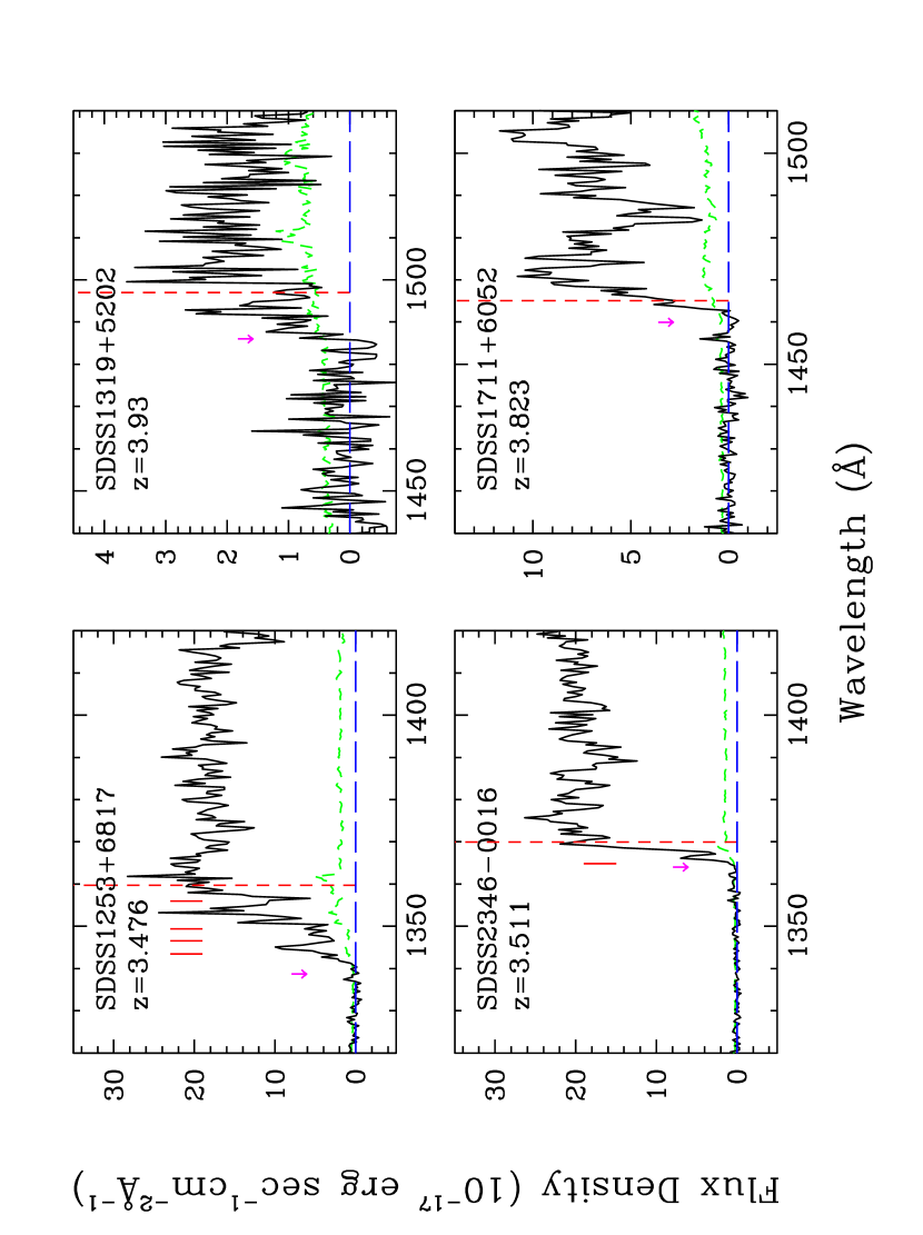
Figure 1:

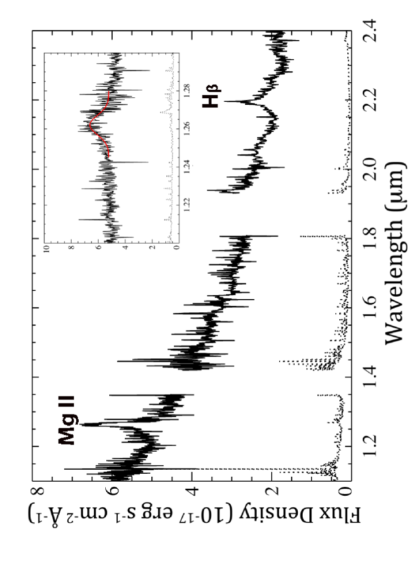
Figure 2:

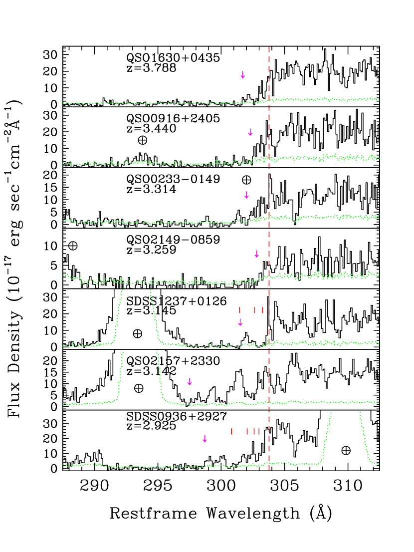
Figure 3:

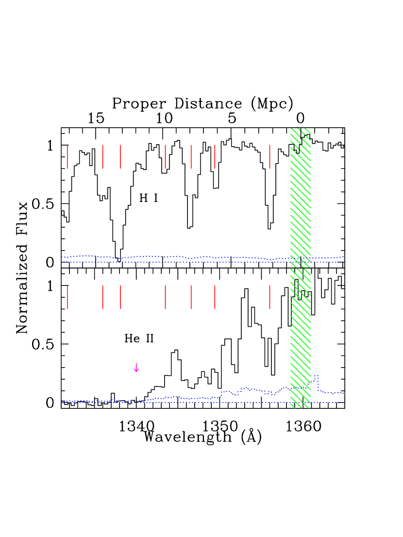
Figure 4:

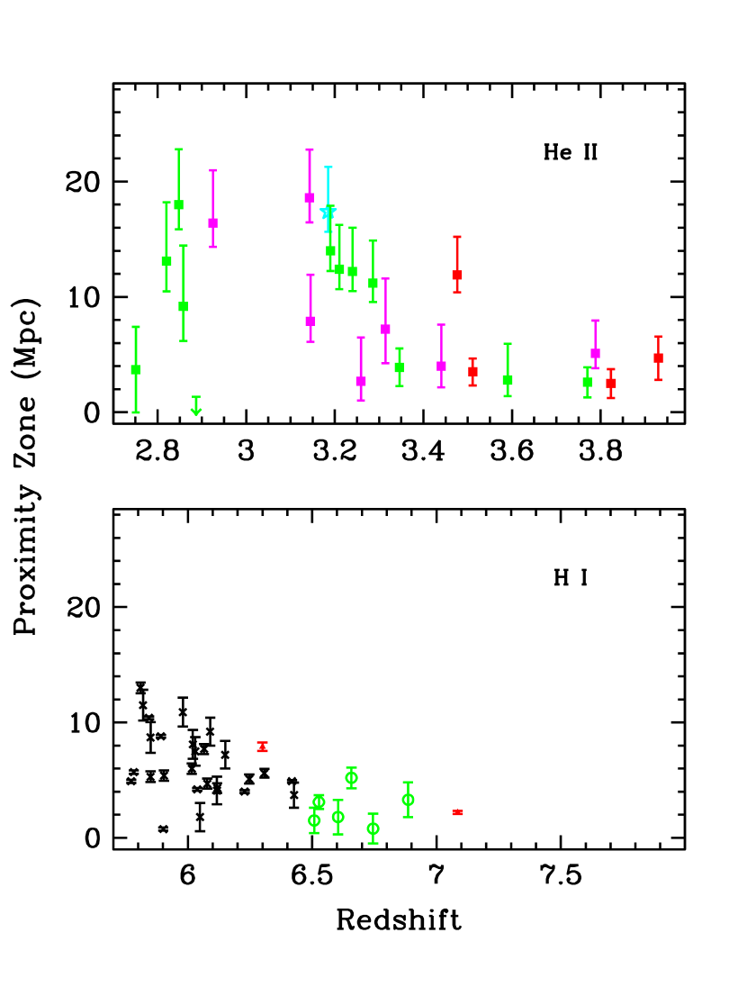
Figure 5:

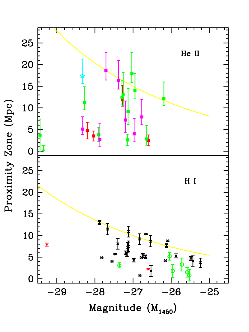
Figure 6:

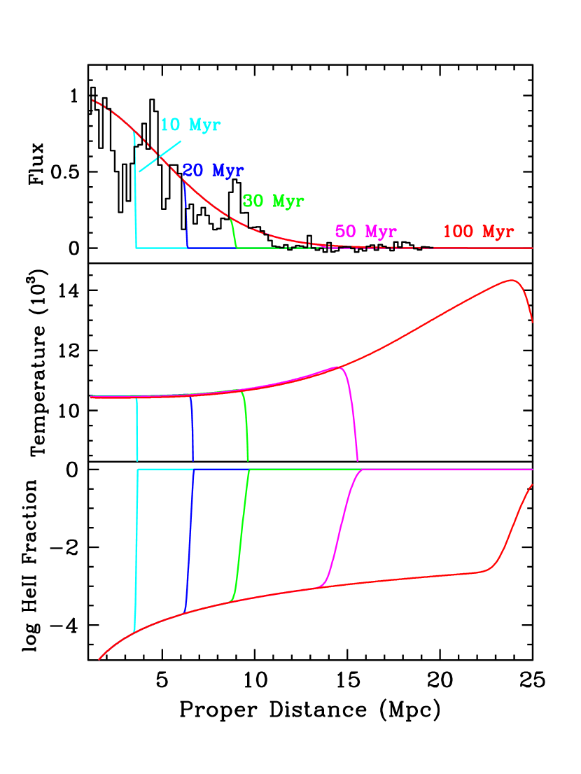
Figure 7:

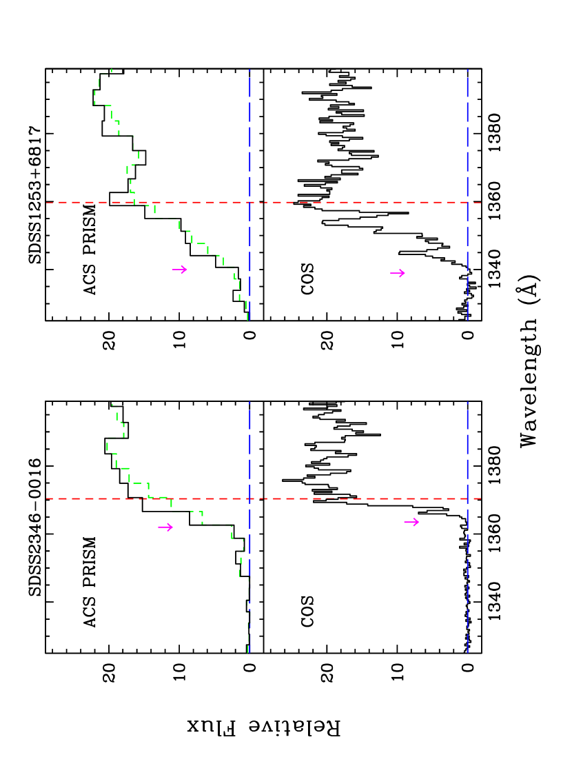
Figure 8:

References

- Anderson et al. (1999) Anderson, S. F., Hogan, C. J., Williams, B. F. & Carswell, R. F. 1999, AJ, 117, 56
- Bajtlik, Duncan & Ostriker (1988) Bajtlik, S., Duncan, R. C. & Ostriker, J. P. 1988, ApJ, 327, 570
- Becker et al. (2013) Becker, G. D., Hewett, P. C., Worseck, G., & Prochaska, J. X. 2013, MNRAS, 430, 2067
- Becker et al. (2001) Becker, R. H., Fan, X., White, R. L. et al. 2001, AJ, 122, 2850
- Carilli et al. (2010) Carilli, C. L., Wang, R., Fan, X. et al. 2010, ApJ, 714, 834
- Carswell et al. (1987) Carswell, R. F., Webb, J. K., Baldwin, J. A. & Atwood, B. 1987, ApJ, 319, 709
- Cen & Haiman (2000) Cen, R. & Haiman, Z. 2000, ApJ, 542, 75
- Dall’Aglio, Wisotzki, & Worseck (2008a) Dall’Aglio, A., Wisotzki, L., & Worseck, G. 2008a, A&A, 480, 359
- Dall’Aglio, Wisotzki, & Worseck (2008b) , 2008b, A&A, 491, 465
- Davidsen, Kriss & Zheng (1996) Davidsen, A. F., Kriss, G. A. & Zheng, W. 1996, Nature 380, 47
- Donahue & Shull (1987) Donahue, M. & Shull, J. M. 1987, ApJ, 323, L13
- Fan, Carilli & Keating (2006) Fan, X., Carilli, C. L., & Keating, B., 2006, ARAA, 44, 415
- Fardal, Giroux & Shull (1998) Fardal, M. A., Giroux, M. L., & Shull, J. M., 1998, AJ, 115, 2206
- Fechner et al. (2004) Fechner, C., Baade, R., & Reimers, D. 2004, A&A, 418, 857
- Fechner et al. (2006) Fechner, C., Reimers, D., Kriss, G, A. et al. 2006, A&A, 455, 91
- Feldman et al. (1992) Feldman, P. D., Davidsen, A. F., Blair, W. P. et al. 1992, Geophy. Rev. Lett., 19, 453
- Fitzpatrick (1999) Fitzpatrick, E. L. 1999, PASP, 111, 63
- Giroux, Fardal & Shull (1995) Giroux, M. L., Fardal, A. A., & Shull, J. M. 1995, ApJ, 451, 477
- Green et al. (2012) Green, J. C., Froning, C. S., Osterman, S. et al. 2012, ApJ, 744, 60
- Gunn & Peterson (1965) Gunn, J. & Peterson, B. 1965, ApJ, 142, 1633
- Haardt & Madau (1996) Haardt, F. & Madau, P. 1996, ApJ, 461, 20
- Heap et al. (2000) Heap, S. R., Williger, G. M., Smette, A. et al. 2000, ApJ, 534, 69
- Hewett & Wild (2010) Hewett, P. C. & Wild, V. 2010, MNRAS, 405, 2302
- Hodge (2011) Hodge, P. E. 2011, in Astronomical Data Analysis Software and Systems XX, eds. I. N. Evans, A. Accomazzi, D. J. Mink, & A. H. Rots, (A. S. P. Conf. Series 442, ASP, San Francisco), 391