Abstract

In this article, we study the charmed baryon states $\Lambda_{c}(2625)$ and $\Xi_{c}(2815)$ with the spin-parity ${3\over 2}^{-}$ by subtracting the contributions from the corresponding charmed baryon states with the spin-parity ${3\over 2}^{+}$ using the QCD sum rules, and suggest a formula $\mu=\sqrt{M_{\Lambda_{c}/\Xi_{c}}^{2}-{\mathbb{M}}_{c}^{2}}$ with the effective mass ${\mathbb{M}}_{c}=1.8\,\rm{GeV}$ to determine the energy scales of the QCD spectral densities, and make reasonable predictions for the masses and pole residues. The numerical results indicate that the $\Lambda_{c}(2625)$ and $\Xi_{c}(2815)$ have at least two remarkable under-structures.

PACS number: 14.20.Lq

Key words: Charmed baryon states, QCD sum rules

1 Introduction

In the past years, several new charmed baryon states have been observed, and the spectroscopy of the charmed baryon states have re-attracted much attentions. The ${1\over 2}^{+}$ and ${1\over 2}^{-}$ antitriplet charmed baryon states ($\Lambda_{c}^{+},\Xi_{c}^{+},\Xi_{c}^{0})$ and ($\Lambda_{c}^{+}(2595),\Xi_{c}^{+}(2790),\Xi_{c}^{0}(2790))$, and the ${1\over 2}^{+}$ and ${3\over 2}^{+}$ sextet charmed baryon states ($\Omega_{c},\Sigma_{c},\Xi^{\prime}_{c}$) and ($\Omega_{c}^{*},\Sigma_{c}^{*},\Xi^{*}_{c}$) have been observed [1]. Now we list out all the charmed baryon states from the particle data group. The $\Lambda^{+}_{c}$, $\Lambda_{c}^{+}(2595)$, $\Lambda_{c}^{+}(2625)$, $\Lambda_{c}^{+}(2765)$ (or $\Sigma_{c}^{+}(2765)$), $\Lambda_{c}^{+}(2880)$ and $\Lambda_{c}^{+}(2940)$ have the spin-parity $J^{P}={\frac{1}{2}}^{+}$, ${\frac{1}{2}}^{-}$, ${\frac{3}{2}}^{-}$, $?$, ${\frac{5}{2}}^{+}$ and $?$, respectively [1]. The $\Xi_{c}$, $\Xi^{\prime}_{c}$, $\Xi_{c}(2645)$, $\Xi_{c}(2790)$, $\Xi_{c}(2815)$, $\Xi_{c}(2980)$, $\Xi_{c}(3055)$, $\Xi_{c}(3080)$ and $\Xi_{c}(3123)$ have the spin-parity ${\frac{1}{2}}^{+}$, ${\frac{1}{2}}^{+}$, ${\frac{3}{2}}^{+}$, ${\frac{1}{2}}^{-}$, ${\frac{3}{2}}^{-}$, $?$, $?$, $?$ and $?$, respectively [1]. The $\Sigma_{c}(2455)$, $\Sigma_{c}(2520)$ and $\Sigma_{c}(2800)$ have the spin-parity ${\frac{1}{2}}^{+}$, ${\frac{3}{2}}^{+}$ and $?$, respectively [1]. The $?$ denotes that the spin-parity is undetermined.

There have been several methods to study the heavy baryon states, such as the QCD sum rules [2, 3, 4, 5, 6, 7, 8, 9, 10], the lattice QCD [11, 12], the relativistic quark model [13], the relativized potential quark model [14], the Feynman-Hellmann theorem [15], the combined expansion in $1/m_{Q}$ and $1/N_{c}$ [16], the hyperfine interaction [17], the variational approach [18], the Faddeev approach [19], the unitarized theory (or model) [20], etc.

In Refs.[5, 6, 7, 8, 9, 10], we study the ${1\over 2}^{\pm}$ and ${3\over 2}^{\pm}$ heavy, doubly-heavy and triply-heavy baryon states in a systematic way with the QCD sum rules by subtracting the contributions from the corresponding ${1\over 2}^{\mp}$ and ${3\over 2}^{\mp}$ heavy, doubly-heavy and triply-heavy baryon states, and make reasonable predictions for their masses and pole residues. For the heavy baryon states $\Lambda_{c}$ and $\Xi_{c}$, the predictions $M_{\Lambda_{c}}=(2.26\pm 0.27)\,\rm{GeV}$, $M_{\Lambda_{c}(2595)}=(2.61\pm 0.21)\,\rm{GeV}$, $M_{\Xi_{c}}=(2.44\pm 0.23)\,\rm{GeV}$, $M_{\Xi^{\prime}_{c}}=(2.56\pm 0.22)\,\rm{GeV}$, $M_{\Xi_{c}(2645)}=(2.65\pm 0.20)\,\rm{GeV}$, $M_{\Xi_{c}(2790)}=(2.76\pm 0.18)\,\rm{GeV}$ and $M_{\Xi_{c}(2815)}=(2.86\pm 0.17)\,\rm{GeV}$ are in good agreement with the experimental data [5, 6, 7, 8], where we take the $\Lambda_{c}(2595)$, $\Xi_{c}(2645)$, $\Xi_{c}(2790)$ and $\Xi_{c}(2815)\,\rm{GeV}$ to be the $\Lambda$-type, $\Sigma$-type, $\Lambda$-type and $\Sigma$-type baryon states, respectively. In the diquark-quark model for the baryons, if the two quarks in the diquark are in relative S-wave, then the baryons with the $0^{+}$ and $1^{+}$ diquarks (the ground state diquarks) are called $\Lambda$-type and $\Sigma$-type baryons respectively. On the other hand, if there exists a relative P-wave between the two quarks in the diquark, then the baryons with the $J^{P}=1^{+}\otimes 1^{-}$ and $0^{+}\otimes 1^{-}$ diquarks are called $\Lambda$-type and $\Sigma$-type baryons respectively, where the $J^{P}=1^{-}$ denotes the relative P-wave, the $0^{+}$ and $1^{+}$ denote the spin-parity of the ground state diquarks.

The flux-tube model favors to assign the $\Lambda^{+}_{c}$, $\Lambda_{c}^{+}(2595)$, $\Lambda_{c}^{+}(2625)$, $\Lambda_{c}^{+}(2765)$ (or $\Sigma_{c}^{+}(2765)$), $\Lambda_{c}^{+}(2880)$ and $\Lambda_{c}^{+}(2940)$ with the spin-parity ${\frac{1}{2}}^{+}$, ${\frac{1}{2}}^{-}$, ${\frac{3}{2}}^{-}$, ${\frac{3}{2}}^{+}$, ${\frac{5}{2}}^{+}$ and ${\frac{5}{2}}^{-}$, respectively [21]. In the non-relativistic quark model [18], the $\Xi_{c}(2790)$ and $\Xi_{c}(2815)$ with the spin-parity ${\frac{1}{2}}^{-}$ and ${\frac{3}{2}}^{-}$ respectively are assigned to be the charmed-strange analogues of the $\Lambda_{c}^{+}(2595)$ and $\Lambda_{c}^{+}(2625)$, or of the $\Lambda(1405)$ and $\Lambda(1520)$; i.e. they are flavor antitriplet or $\Lambda$-type heavy baryon states. In the relativistic quark model [13], the $\Xi_{c}(2815)$ also is taken to be the $\Lambda$-type baryon state.

The $\Xi_{c}(2815)$ may be the $\Lambda$-type or $\Sigma$-type baryon state with the spin-parity ${\frac{3}{2}}^{-}$, there are two possibilities, while the $\Xi_{c}(2980)$, $\Xi_{c}(3055)$, $\Xi_{c}(3080)$ and $\Xi_{c}(3123)$ are unlikely the ground state ${\frac{3}{2}}^{-}$ states due to their large masses. In this article, we will focus on the possible assignments of the $\Lambda_{c}(2625)$ and $\Xi_{c}(2815)$ to be the $\Lambda$-type baryon states. In previous work, we take the $\Xi_{c}(2815)$ to be the $\Sigma$-type baryon state [8].

We usually resort to the diquark-quark model to construct the baryon currents. Without introducing additional P-wave, the ground state quarks have the spin-parity ${1\over 2}^{+}$, two quarks can form a scalar diquark or an axialvector diquark with the spin-parity $0^{+}$ or $1^{+}$, the diquark then combines with a third quark to form a positive parity baryon,

$$\left[{1\over 2}^{+}\otimes{1\over 2}^{+}\right]\otimes{1\over 2}^{+} = \left[{0}^{+}\oplus{1}^{+}\right]\otimes{1\over 2}^{+}={1\over 2}^{+}\oplus{1\over 2}^{+}\oplus{3\over 2}^{+}\,,$$ (1)

for example, the $\Lambda$-type currents $\eta^{\Lambda}$,

$$\eta^{\Lambda} = \varepsilon^{abc}q^{T}_{a}C\gamma_{5}q^{\prime}_{b}\,Q_{c},$$ (2)

the $\Sigma$-type currents $\eta^{\Sigma}$ and $\eta^{\Sigma}_{\mu}$,

$$\eta^{\Sigma} = \varepsilon^{abc}q^{T}_{a}C\gamma_{\mu}q^{\prime}_{b}\,\gamma^{\mu}\gamma_{5}Q_{c}\,,$$

$$\eta^{\Sigma}_{\mu} = \varepsilon^{abc}q^{T}_{a}C\gamma_{\mu}q^{\prime}_{b}\,Q_{c}\,,$$ (3)

which have positive parity, where the $a$, $b$ and $c$ are color indices. Multiplying $i\gamma_{5}$ to the currents $\eta^{\Lambda}$, $\eta^{\Sigma}$ and $\eta^{\Sigma}_{\mu}$ changes their parity, the currents $i\gamma_{5}\eta^{\Lambda}$, $i\gamma_{5}\eta^{\Sigma}$ and $i\gamma_{5}\eta^{\Sigma}_{\mu}$ couple potentially to the negative parity heavy baryons. In Refs.[6, 8, 10], we take the currents without introducing partial (or P-wave) to study the negative parity heavy, doubly-heavy and triply-heavy baryon states, and obtain satisfactory results.

If there exists a relative P-wave (which can be denoted as $1^{-}$) between the diquark and the third quark or between the two quarks in the diquark, we have the following two routines to construct the negative parity baryons,

$$\left[{1\over 2}^{+}\otimes{1\over 2}^{+}\right]\otimes\left({1\over 2}^{+}\otimes{1^{-}}\right) = \left[{0}^{+}\oplus{1}^{+}\right]\otimes\left({1\over 2}^{-}\oplus{3\over 2}^{-}\right)\,,$$ (4)

and

$$\left[\left({1\over 2}^{+}\otimes{1^{-}}\right)\otimes{1\over 2}^{+}\right]\otimes{1\over 2}^{+} = \left[\left({1\over 2}^{-}\oplus{3\over 2}^{-}\right)\otimes{1\over 2}^{+}\right]\otimes{1\over 2}^{+}$$ (5)

$$= \left[0^{-}\oplus 1^{-}\oplus 1^{-}\oplus 2^{-}\right]\otimes{1\over 2}^{+}\,,$$

or equivalently

$$\left[\left({1\over 2}^{+}\otimes{1\over 2}^{+}\right)\otimes{1^{-}}\right]\otimes{1\over 2}^{+} = \left[\left(0^{+}\oplus 1^{+}\right)\otimes 1^{-}\right]\otimes{1\over 2}^{+}$$ (6)

$$= \left[1^{-}\oplus 0^{-}\oplus 1^{-}\oplus 2^{-}\right]\otimes{1\over 2}^{+}\,.$$

Recently, Chen et al introduce the relative P-wave explicitly, and study the negative parity charmed baryon states with the QCD sum rules combined with the heavy quark effective theory [22]. The baryons have complicated structures, more than one currents can couple potentially to a special baryon. In this article, we construct the interpolating currents by introducing the relative P-wave explicitly, and study the negative parity charmed baryon states $\Lambda_{c}(2625)$ and $\Xi_{c}(2815)$ with the full QCD sum rules.

In Ref.[23], Jido, Kodama and Oka suggest a novel method to separate the contribution of the negative-parity baryon $N(1535)$ from that of the positive-parity baryon $p$, because the interpolating currents maybe couple potentially to both the negative- and positive-parity baryon states [24], which impairs the predictive power. Again, we follow this novel method to study the negative-parity baryon states $\Lambda_{c}(2625)$ and $\Xi_{c}(2815)$ by separating the contributions of the positive-parity baryon states explicitly. In the heavy quark limit, Bagan et al separate the contributions of the positive- and negative-parity heavy baryon states unambiguously [25].

The article is arranged as follows: we derive the QCD sum rules for the masses and pole residues of the $\Lambda_{c}(2625)$ and $\Xi_{c}(2815)$ in Sect.2; in Sect.3, we present the numerical results and discussions; and Sect.4 is reserved for our conclusions.

2 QCD sum rules for the $\Lambda_{c}(2625)$ and $\Xi_{c}(2815)$

In the following, we write down the two-point correlation functions $\Pi_{\alpha\beta}(p)$ in the QCD sum rules,

$$\Pi_{\alpha\beta}(p) = i\int d^{4}xe^{ip\cdot x}\langle 0|T\left\{J_{\alpha}(x)\bar{J}_{\beta}(0)\right\}|0\rangle\,,$$ (7)

where $J_{\alpha}(x)=J^{1}_{\alpha}(x),\,J^{2}_{\alpha}(x)$,

$$J^{1}_{\alpha}(x) = i\varepsilon^{ijk}\left[\partial^{\mu}q^{T}_{i}(x)C\gamma^{\nu}q^{\prime}_{j}(x)-q^{T}_{i}(x)C\gamma^{\nu}\partial^{\mu}q^{\prime}_{j}(x)\right]\left(\widetilde{g}_{\alpha\mu}\gamma_{\nu}-\widetilde{g}_{\alpha\nu}\gamma_{\mu}\right)\gamma_{5}c_{k}(x)\,,$$ (8)

$$J^{2}_{\alpha}(x) = i\varepsilon^{ijk}\left[\partial^{\mu}q^{T}_{i}(x)C\gamma^{\nu}q^{\prime}_{j}(x)-q^{T}_{i}(x)C\gamma^{\nu}\partial^{\mu}q^{\prime}_{j}(x)\right]\left(g_{\alpha\mu}\gamma_{\nu}+g_{\alpha\nu}\gamma_{\mu}-\frac{1}{2}g_{\mu\nu}\gamma_{\alpha}\right)\gamma_{5}c_{k}(x)\,,$$

$\widetilde{g}_{\mu\nu}=g_{\mu\nu}-\frac{1}{4}\gamma_{\mu}\gamma_{\nu}$, the $i$, $j$, $k$ are color indices, the $C$ is the charge conjugation matrix. The light diquark constituents $\varepsilon^{ijk}\left[\partial^{\mu}q^{T}_{i}(x)C\gamma^{\nu}q^{\prime}_{j}(x)-q^{T}_{i}(x)C\gamma^{\nu}\partial^{\mu}q^{\prime}_{j}(x)\right]$ in the currents $J_{\alpha}$ have the same formula, i.e. they have the two Lorentz indices $\mu$ and $\nu$, and couple potentially to the spin-1 or 2 diquarks. The Dirac matrixes $\widetilde{g}_{\alpha\mu}\gamma_{\nu}-\widetilde{g}_{\alpha\nu}\gamma_{\mu}$ and $g_{\alpha\mu}\gamma_{\nu}+g_{\alpha\nu}\gamma_{\mu}-\frac{1}{2}g_{\mu\nu}\gamma_{\alpha}$ are anti-symmetric and symmetric respectively when interchanging the indices $\mu$ and $\nu$, which are contracted with the corresponding indices in the diquark constituents, so the diquark constituents in the currents $J_{\alpha}^{1}$ and $J^{2}_{\alpha}$ have the spins 1 and 2, respectively. Furthermore, the currents $J^{1}_{\alpha}$ and $J^{2}_{\alpha}$ both have negative parity. We use the currents $J_{\alpha}$ with $q=u$ and $q^{\prime}=d$ ($q=u$ and $q^{\prime}=s$ or $q=d$ and $q^{\prime}=s$) to interpolate the $\Lambda_{c}(2625)$ ($\Xi_{c}(2815)$).

The currents $J_{\alpha}(0)$ couple potentially to the ${\frac{3}{2}}^{-}$ charmed baryon states $B^{-}$,

$$\langle 0|J_{\alpha}(0)|B^{-}(p)\rangle = \lambda_{-}U^{-}_{\alpha}(p,s)\,,$$ (10)

the spinor $U^{-}_{\alpha}(p,s)$ satisfies the Rarita-Schwinger equation $(\not\!\!p-M_{-})U^{-}_{\alpha}(p)=0$ and the relations $\gamma^{\alpha}U^{-}_{\alpha}(p,s)=0$, $p^{\alpha}U^{-}_{\alpha}(p,s)=0$. The currents also satisfy the relation $\gamma^{\alpha}J_{\alpha}(x)=0$, which is consistent with Eq.(10). On the other hand, the currents also couple to the positive parity baryon states $B^{+}$,

$$\langle 0|J_{\alpha}(0)|B^{+}(p)\rangle = \lambda_{+}i\gamma_{5}U^{+}_{\alpha}(p,s)\,,$$ (11)

the spinors $U^{\pm}_{\alpha}(p,s)$ have analogous properties and $\lambda_{+}\neq 0$.

We insert a complete set of intermediate baryon states with the same quantum numbers as the current operators $J_{\alpha}(x)$ and $i\gamma_{5}J_{\alpha}(x)$ into the correlation functions $\Pi_{\alpha\beta}(p)$ to obtain the hadronic representation [26, 27]. After isolating the pole terms of the lowest states of the charmed baryons, we obtain the following results:

$$\Pi_{\alpha\beta}(p) = \lambda_{-}^{2}{\!\not\!{p}+M_{-}\over M_{-}^{2}-p^{2}}\left(-g_{\alpha\beta}+\frac{\gamma_{\alpha}\gamma_{\beta}}{3}+\frac{2p_{\alpha}p_{\beta}}{3M_{-}^{2}}-\frac{p_{\alpha}\gamma_{\beta}-p_{\beta}\gamma_{\alpha}}{3M_{-}}\right)+$$ (12)

$$\lambda_{+}^{2}{\!\not\!{p}-M_{+}\over M^{2}_{+}-p^{2}}\left(-g_{\alpha\beta}+\frac{\gamma_{\alpha}\gamma_{\beta}}{3}+\frac{2p_{\alpha}p_{\beta}}{3M_{+}^{2}}-\frac{p_{\alpha}\gamma_{\beta}-p_{\beta}\gamma_{\alpha}}{3M_{+}}\right)+\cdots$$

$$= \Pi(p)\left(-g_{\alpha\beta}\right)+\cdots\,,$$

where the $M_{\pm}$ are the masses of the lowest states with the parity $\pm$ respectively, and the $\lambda_{\pm}$ are the corresponding pole residues (or couplings). In this article, we choose the tensor structure $g_{\mu\nu}$ for analysis. If we take $\vec{p}=0$, then

$$\rm{limit}_{\epsilon\rightarrow 0}\frac{{\rm Im}\Pi(p_{0}+i\epsilon)}{\pi} = \lambda_{-}^{2}{\gamma_{0}+1\over 2}\delta(p_{0}-M_{-})+\lambda_{+}^{2}{\gamma_{0}-1\over 2}\delta(p_{0}-M_{+})+\cdots$$ (13)

$$= \gamma_{0}A(p_{0})+B(p_{0})+\cdots\,,$$

where

$$A(p_{0}) = {1\over 2}\left[\lambda_{-}^{2}\delta(p_{0}-M_{-})+\lambda_{+}^{2}\delta(p_{0}-M_{+})\right]\,,$$

$$B(p_{0}) = {1\over 2}\left[\lambda_{-}^{2}\delta(p_{0}-M_{-})-\lambda_{+}^{2}\delta(p_{0}-M_{+})\right]\,,$$ (14)

the $A(p_{0})+B(p_{0})$ and $A(p_{0})-B(p_{0})$ contain the contributions from the negative- and positive-parity baryon states, respectively [23].

We calculate the light quark parts of the correlation functions $\Pi_{\alpha\beta}(p)$ with the full light quark propagators in the coordinate space and use the momentum space expression for the $c$-quark propagator,

$$S_{ij}(x) = \frac{i\delta_{ij}\!\not\!{x}}{2\pi^{2}x^{4}}-\frac{\delta_{ij}m_{q}}{4\pi^{2}x^{2}}-\frac{\delta_{ij}\langle\bar{q}q\rangle}{12}+\frac{i\delta_{ij}\!\not\!{x}m_{q}\langle\bar{q}q\rangle}{48}-\frac{\delta_{ij}x^{2}\langle\bar{q}g_{s}\sigma Gq\rangle}{192}+\frac{i\delta_{ij}x^{2}\!\not\!{x}m_{q}\langle\bar{q}g_{s}\sigma Gq\rangle}{1152}$$ (15)

$$-\frac{ig_{s}G^{a}_{\alpha\beta}t^{a}_{ij}(\!\not\!{x}\sigma^{\alpha\beta}+\sigma^{\alpha\beta}\!\not\!{x})}{32\pi^{2}x^{2}}-\frac{1}{8}\langle\bar{q}_{j}\sigma^{\mu\nu}q_{i}\rangle\sigma_{\mu\nu}+\cdots\,,$$

$$C_{ij}(x) = \frac{i}{(2\pi)^{4}}\int d^{4}ke^{-ik\cdot x}\left\{\frac{\delta_{ij}}{\!\not\!{k}-m_{c}}-\frac{g_{s}G^{n}_{\alpha\beta}t^{n}_{ij}}{4}\frac{\sigma^{\alpha\beta}(\!\not\!{k}+m_{c})+(\!\not\!{k}+m_{c})\sigma^{\alpha\beta}}{(k^{2}-m_{c}^{2})^{2}}\right.$$

$$\left.-\frac{g_{s}^{2}(t^{a}t^{b})_{ij}G^{a}_{\alpha\beta}G^{b}_{\mu\nu}(f^{\alpha\beta\mu\nu}+f^{\alpha\mu\beta\nu}+f^{\alpha\mu\nu\beta})}{4(k^{2}-m_{c}^{2})^{5}}+\cdots\right\}\,,$$

$$f^{\alpha\beta\mu\nu} = (\!\not\!{k}+m_{c})\gamma^{\alpha}(\!\not\!{k}+m_{c})\gamma^{\beta}(\!\not\!{k}+m_{c})\gamma^{\mu}(\!\not\!{k}+m_{c})\gamma^{\nu}(\!\not\!{k}+m_{c})\,,$$ (16)

and $t^{n}=\frac{\lambda^{n}}{2}$, the $\lambda^{n}$ is the Gell-Mann matrix [27]. We contract the quark fields in the correlation functions and take the full light-quark and heavy-quark propagators firstly, then compute the integrals both in the coordinate and momentum spaces, and obtain the correlation functions $\Pi_{\alpha\beta}(p)$ therefore the QCD spectral densities through dispersion relation, the explicit expression are give in the appendix. In Eq.(15), we retain the term $\langle\bar{q}_{j}\sigma_{\mu\nu}q_{i}\rangle$ originates from the Fierz re-arrangement of the $\langle q_{i}\bar{q}_{j}\rangle$ to absorb the gluons emitted from the other quark lines to form $\langle\bar{q}_{j}g_{s}G^{a}_{\alpha\beta}t^{a}_{mn}\sigma_{\mu\nu}q_{i}\rangle$ so as to extract the mixed condensate $\langle\bar{q}g_{s}\sigma Gq\rangle$. Finally we introduce the weight functions $\exp\left(-\frac{p_{0}^{2}}{T^{2}}\right)$, $p_{0}^{2}\exp\left(-\frac{p_{0}^{2}}{T^{2}}\right)$, and obtain the following QCD sum rules,

$$\lambda_{-}^{2}\exp\left(-\frac{M_{-}^{2}}{T^{2}}\right) = \int_{m_{c}}^{\sqrt{s_{0}}}dp_{0}\left[\rho^{A}(p_{0})+\rho^{B}(p_{0})\right]\exp\left(-\frac{p_{0}^{2}}{T^{2}}\right)\,,$$ (17)

$$\lambda_{-}^{2}M_{-}^{2}\exp\left(-\frac{M_{-}^{2}}{T^{2}}\right) = \int_{m_{c}}^{\sqrt{s_{0}}}dp_{0}\left[\rho^{A}(p_{0})+\rho^{B}(p_{0})\right]p_{0}^{2}\exp\left(-\frac{p_{0}^{2}}{T^{2}}\right)\,,$$ (18)

where the $s_{0}$ are the continuum threshold parameters and the $T^{2}$ are the Borel parameters. The QCD spectral densities $\rho^{A}(p_{0})$ and $\rho^{B}(p_{0})$ are given explicitly in the Appendix.

3 Numerical results and discussions

The vacuum condensates are taken to be the standard values $\langle\bar{q}q\rangle=-(0.24\pm 0.01\,\rm{GeV})^{3}$, $\langle\bar{s}s\rangle=(0.8\pm 0.1)\langle\bar{q}q\rangle$, $\langle\bar{q}g_{s}\sigma Gq\rangle=m_{0}^{2}\langle\bar{q}q\rangle$, $\langle\bar{s}g_{s}\sigma Gs\rangle=m_{0}^{2}\langle\bar{s}s\rangle$, $m_{0}^{2}=(0.8\pm 0.1)\,\rm{GeV}^{2}$, $\langle\frac{\alpha_{s}GG}{\pi}\rangle=(0.33\,\rm{GeV})^{4}$ at the energy scale $\mu=1\,\rm{GeV}$ [26, 27, 28]. The quark condensate and mixed quark condensate evolve with the renormalization group equation, $\langle\bar{q}q\rangle(\mu)=\langle\bar{q}q\rangle(Q)\left[\frac{\alpha_{s}(Q)}{\alpha_{s}(\mu)}\right]^{\frac{4}{9}}$, $\langle\bar{s}s\rangle(\mu)=\langle\bar{s}s\rangle(Q)\left[\frac{\alpha_{s}(Q)}{\alpha_{s}(\mu)}\right]^{\frac{4}{9}}$, $\langle\bar{q}g_{s}\sigma Gq\rangle(\mu)=\langle\bar{q}g_{s}\sigma Gq\rangle(Q)\left[\frac{\alpha_{s}(Q)}{\alpha_{s}(\mu)}\right]^{\frac{2}{27}}$ and $\langle\bar{s}g_{s}\sigma Gs\rangle(\mu)=\langle\bar{s}g_{s}\sigma Gs\rangle(Q)\left[\frac{\alpha_{s}(Q)}{\alpha_{s}(\mu)}\right]^{\frac{2}{27}}$.

In the article, we take the $\overline{MS}$ masses $m_{c}(m_{c})=(1.275\pm 0.025)\,\rm{GeV}$ and $m_{s}(\mu=2\,\rm{GeV})=(0.095\pm 0.005)\,\rm{GeV}$ from the particle data group [1], and take into account the energy-scale dependence of the $\overline{MS}$ masses from the renormalization group equation,

$$m_{c}(\mu) = m_{c}(m_{c})\left[\frac{\alpha_{s}(\mu)}{\alpha_{s}(m_{c})}\right]^{\frac{12}{25}}\,,$$

$$m_{s}(\mu) = m_{s}({\rm 2GeV})\left[\frac{\alpha_{s}(\mu)}{\alpha_{s}({\rm 2GeV})}\right]^{\frac{4}{9}}\,,$$

$$\alpha_{s}(\mu) = \frac{1}{b_{0}t}\left[1-\frac{b_{1}}{b_{0}^{2}}\frac{\log t}{t}+\frac{b_{1}^{2}(\log^{2}{t}-\log{t}-1)+b_{0}b_{2}}{b_{0}^{4}t^{2}}\right]\,,$$ (19)

where $t=\log\frac{\mu^{2}}{\Lambda^{2}}$, $b_{0}=\frac{33-2n_{f}}{12\pi}$, $b_{1}=\frac{153-19n_{f}}{24\pi^{2}}$, $b_{2}=\frac{2857-\frac{5033}{9}n_{f}+\frac{325}{27}n_{f}^{2}}{128\pi^{3}}$, $\Lambda=213\,\rm{MeV}$, $296\,\rm{MeV}$ and $339\,\rm{MeV}$ for the flavors $n_{f}=5$, $4$ and $3$, respectively [1].

In Refs.[29, 30, 31], we study the acceptable energy scales of the QCD spectral densities for the hidden charmed (bottom) tetraquark states and molecular (and molecule-like) states in the QCD sum rules in details for the first time, and suggest a formula $\mu=\sqrt{M^{2}_{X/Y/Z}-(2{\mathbb{M}}_{Q})^{2}}$ to determine the energy scales, where the $X$, $Y$, $Z$ denote the four-quark systems, and the ${\mathbb{M}}_{Q}$ is the effective heavy quark mass. We can describe the system $Q\bar{Q}q^{\prime}\bar{q}$ by a double-well potential with two light quarks $q^{\prime}\bar{q}$ lying in the two wells respectively. In the heavy quark limit, the $Q$-quark serves as a static well potential and bounds the light quark $q^{\prime}$ to form a diquark in the color antitriplet channel or binds the light antiquark $\bar{q}$ to form a meson (or meson-like) in the color singlet (or octet) channel. Then the four-quark systems are characterized by the effective masses ${\mathbb{M}}_{Q}$ and the virtuality $V=\sqrt{M^{2}_{X/Y/Z}-(2{\mathbb{M}}_{Q})^{2}}$. We assume $\mu^{2}=V^{2}={\mathcal{O}}(T^{2})$, the effective mass ${\mathbb{M}}_{c}=1.8\,\rm{GeV}$ is the optimal value for the diquark-antidiquark type tetraquark states [29, 30]. In this article, we use the diquark-quark model to construct the interpolating currents, and take the analogous formula,

$$\mu = \sqrt{M_{\Lambda_{c}/\Xi_{c}}^{2}-{\mathbb{M}}_{c}^{2}}\,,$$ (20)

with the value ${\mathbb{M}}_{c}=1.8\,\rm{GeV}$ to determine the energy scales of the QCD spectral densities. Then we obtain the values $\mu=1.9\,\rm{GeV}$ and $\mu=2.2\,\rm{GeV}$ for the $\Lambda_{c}(2625)$ and $\Xi_{c}(2815)$, respectively.

In the conventional QCD sum rules [26, 27], we usually use two criteria (pole dominance and convergence of the operator product expansion) to choose the Borel parameters $T^{2}$ and continuum threshold parameters $s_{0}$. In Refs.[5, 6, 7, 8, 9, 10], we study the ${1\over 2}^{\pm}$ and ${3\over 2}^{\pm}$ heavy, doubly-heavy and triply-heavy baryon states in a systematic way with the QCD sum rules by subtracting the contributions from the corresponding ${1\over 2}^{\mp}$ and ${3\over 2}^{\mp}$ heavy, doubly-heavy and triply-heavy baryon states, the continuum threshold parameters $\sqrt{s_{0}}-M_{\rm{gr}}\approx(0.6-0.8)\,\rm{GeV}$ can lead to satisfactory results, where $M_{\rm{gr}}$ denotes the ground state masses. The masses of the $\Lambda_{c}(2625)$ and $\Xi_{c}(2815)$ are $M_{\Lambda_{c}(2625)}=(2628.11\pm 0.19)\,\rm{MeV}$, $M_{\Xi^{+}_{c}(2815)}=(2816.6\pm 0.9)\,\rm{MeV}$ and $M_{\Xi^{0}_{c}(2815)}=(2819.6\pm 1.2)\,\rm{MeV}$ from the particle data group [1]. In this article, we take the values $\sqrt{s_{0}}\approx M_{\rm gr}+(0.6-0.8)\,\rm{GeV}$, the two criteria of the QCD sum rules are also satisfied, see Table 1. The values $(0.6-0.8)\,\rm{GeV}$ are somewhat larger than the usually used values $(0.4-0.6)\,\rm{GeV}$, there maybe exist some contaminations from the higher resonances. If we take the largest values $\sqrt{s_{0}}=M_{\rm gr}+0.8\,\rm{GeV}$, the upper bound of the factors $\exp\left(-\frac{s_{0}}{T^{2}}\right)$ is about $0.003-0.005$, the contaminations are greatly suppressed and can be neglected safely. In the table, we present the values of the Borel parameters $T^{2}$, continuum threshold parameters $s_{0}$, the pole contributions and the perturbative contributions explicitly.

	$T^{2}(\rm{GeV}^{2})$	$\sqrt{s_{0}}(\rm{GeV})$	pole	perturbative
$\Lambda_{c}(2625)\,\,(J^{1}_{\alpha})$	$1.6-2.0$	$3.3$	$(50-72)\%$	$(81-95)\%$
$\Lambda_{c}(2625)\,\,(J^{2}_{\alpha})$	$1.8-2.2$	$3.3$	$(45-65)\%$	$(76-88)\%$
$\Xi_{c}(2815)\,\,(J^{1}_{\alpha})$	$1.6-2.2$	$3.5$	$(54-82)\%$	$\geq 89\%$
$\Xi_{c}(2815)\,\,(J^{2}_{\alpha})$	$1.8-2.4$	$3.5$	$(50-75)\%$	$(82-94)\%$

Table 1: The Borel parameters $T^{2}$, continuum threshold parameters $s_{0}$, the pole contributions (pole) and the perturbative contributions (perturbative).

Taking into account all uncertainties of the revelent parameters, we can obtain the values of the masses and pole residues of the $\Lambda_{c}(2625)$ and $\Xi_{c}(2815)$, which are shown in Figs.1-2 and Table 2. From the table, we can see that the values of the masses $M_{\Lambda_{c}(2625)}$ and $M_{\Xi_{c}(2815)}$ can reproduce the experimental data for all the currents $J_{\alpha}^{1}$ and $J_{\alpha}^{2}$. The angular momentums of the light diquarks are $1$ and $2$ in the currents $J_{\alpha}^{1}$ and $J_{\alpha}^{2}$, respectively, they all couple potentially to the baryons $\Lambda_{c}(2625)$ and $\Xi_{c}(2815)$, so the $\Lambda_{c}(2625)$ and $\Xi_{c}(2815)$ have at least two remarkable under-structures.

In previous work [8], we take the $\Xi_{c}(2815)$ to be the $\Sigma$-type baryon state, and study the $\Xi_{c}(2815)$ with the interpolating current $J_{\alpha}^{\Xi}(x)=\epsilon^{ijk}q^{T}_{i}(x)C\gamma_{\alpha}s_{j}(x)c_{k}(x)$ or $J_{\alpha}^{\Xi}(x)=\epsilon^{ijk}q^{T}_{i}(x)C\gamma^{\beta}s_{j}(x)\widetilde{g}_{\alpha\beta}c_{k}(x)$, and obtain the value $M_{\Xi_{c}(2815)}=(2.86\pm 0.17)\,\rm{GeV}$, which is also consistent with the experimental data. If the prediction is robust, now the $\Xi_{c}(2815)$ has at least three remarkable under-structures.

In Fig.3, we plot the masses $M_{\Lambda_{c}(2625)}$ and $M_{\Xi_{c}(2815)}$ with variations of the energy scales $\mu$ for the central values of the other input parameters. From the figure, we can see that the $M_{\Lambda_{c}(2625)}$ and $M_{\Xi_{c}(2815)}$ decrease monotonously but mildly with increase of the energy scales $\mu$, $M_{\Lambda_{c}(2625)}\approx(2.60-2.63)\,\rm{GeV}$ and $M_{\Xi_{c}(2815)}\approx(2.82-2.88)\,\rm{GeV}$ at the energy scales $\mu=(1-3)\,\rm{GeV}$, the allowed energy scales are $\mu_{\Lambda_{c}(2625)}=(1-3)\,\rm{GeV}$ and $\mu_{\Xi_{c}(2815)}=(1.4-3.0)\,\rm{GeV}$, if we assume $M_{\Xi_{c}(2815)}\leq 2.86\,\rm{GeV}$, so the energy scale formula in Eq.(20) works, the formula can be extend to study other heavy baryon states.

	$T^{2}(\rm{GeV}^{2})$	$\sqrt{s_{0}}(\rm{GeV})$	$M(\rm{GeV})$	$\lambda(\rm{GeV}^{4})$
$\Lambda_{c}(2625)\,\,(J^{1}_{\alpha})$	$1.6-2.0$	$3.3\pm 0.1$	$2.62\pm 0.18$	$0.041\pm 0.014$
$\Lambda_{c}(2625)\,\,(J^{2}_{\alpha})$	$1.8-2.2$	$3.3\pm 0.1$	$2.61\pm 0.18$	$0.072\pm 0.022$
$\Xi_{c}(2815)\,\,(J^{1}_{\alpha})$	$1.6-2.2$	$3.5\pm 0.1$	$2.83\pm 0.17$	$0.065\pm 0.022$
$\Xi_{c}(2815)\,\,(J^{2}_{\alpha})$	$1.8-2.4$	$3.5\pm 0.1$	$2.83\pm 0.17$	$0.113\pm 0.034$

Table 2: The masses $M$ and pole residues $\lambda$ of the $\Lambda_{c}(2625)$ and $\Xi_{c}(2815)$.

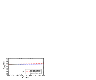
Figure 1: The masses of the $\Lambda_{c}(2625)$ and $\Xi_{c}(2815)$ with variations of the Borel parameters $T^{2}$, where the (I) and (II) denote the currents $J^{1}_{\alpha}$ and $J^{2}_{\alpha}$, respectively.

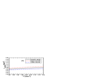
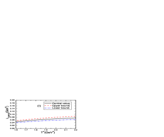
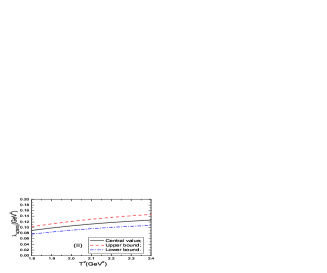
Figure 2: The pole residues of the $\Lambda_{c}(2625)$ and $\Xi_{c}(2815)$ with variations of the Borel parameter $T^{2}$, where the (I) and (II) denote the currents $J^{1}_{\alpha}$ and $J^{2}_{\alpha}$, respectively.

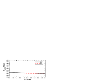
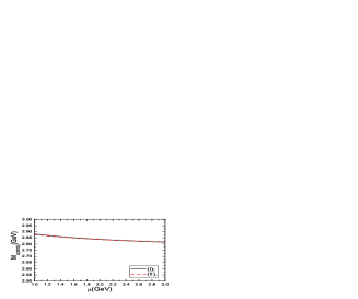
Figure 3: The masses of the $\Lambda_{c}(2625)$ and $\Xi_{c}(2815)$ with variations of the energy scales $\mu$ where the (I) and (II) denote the currents $J^{1}_{\alpha}$ and $J^{2}_{\alpha}$, respectively.

4 Conclusion

In this article, we study the charmed baryon states $\Lambda_{c}(2625)$ and $\Xi_{c}(2815)$ with the spin-parity ${\frac{3}{2}^{-}}$ by subtracting the contributions from the corresponding charmed baryon states with the spin-parity ${\frac{3}{2}^{+}}$ using the QCD sum rules, and suggest an energy scale formula to determine the energy scales of the QCD spectral densities, and make reasonable predictions for their masses and pole residues. The numerical results indicate that the $\Lambda_{c}(2625)$ and $\Xi_{c}(2815)$ at least have two remarkable under-structures. We can take pole residues as basic input parameters and study the revelent hadronic processes with the QCD sum rules in further investigations of the under-structures of the $\Lambda_{c}(2625)$ and $\Xi_{c}(2815)$.

Appendix

The spectral densities of the $\Lambda_{c}(2625)$ and $\Xi_{c}(2815)$ at the quark level,

$$\rho^{A}_{J^{1}_{us}}(p_{0}) = \frac{p_{0}}{192\pi^{4}}\int_{t_{i}}^{1}dt(1-t)^{4}\left(p_{0}^{2}-\widetilde{m}_{c}^{2}\right)^{2}\left[(4-5t)p_{0}^{2}+(2t-1)\widetilde{m}_{c}^{2}\right]$$ (21)

$$+\frac{m_{s}\left[\langle\bar{q}q\rangle-2\langle\bar{s}s\rangle\right]p_{0}}{16\pi^{2}}\int_{t_{i}}^{1}dt(1-t)^{2}\left[(6t-5)p_{0}^{2}+(3-4t)\widetilde{m}_{c}^{2}\right]+$$

$$\frac{m_{s}\left[12\langle\bar{q}g_{s}\sigma Gq\rangle-11\langle\bar{s}g_{s}\sigma Gs\rangle\right]p_{0}}{384\pi^{2}}\int_{t_{i}}^{1}dt(1-t)\left[(7-8t)+2(1-t)p_{0}\delta(p_{0}-\widetilde{m}_{c})\right]$$

$$+\frac{p_{0}m_{c}^{2}}{576\pi^{2}}\langle\frac{\alpha_{s}GG}{\pi}\rangle\int_{t_{i}}^{1}dt\frac{(1-t)^{4}}{t^{3}}\left[2t-1-\frac{(1-t)p_{0}}{2}\delta(p_{0}-\widetilde{m}_{c})\right]$$

$$+\frac{m_{s}\langle\bar{q}g_{s}\sigma Gq\rangle p_{0}}{192\pi^{2}}\int_{t_{i}}^{1}dt\frac{(1-t)^{2}}{t}\left[3-4t+\frac{(1-t)p_{0}}{2}\delta(p_{0}-\widetilde{m}_{c})\right]$$

$$+\frac{p_{0}}{768\pi^{2}}\langle\frac{\alpha_{s}GG}{\pi}\rangle\int_{t_{i}}^{1}dt\frac{(1-t)^{3}}{t}\left[(10t-7)p_{0}^{2}+(5-8t)\widetilde{m}_{c}^{2}\right]\,,$$

$$\rho^{B}_{J^{1}_{us}}(p_{0}) = \frac{m_{c}}{128\pi^{4}}\int_{t_{i}}^{1}dt(1-t)^{3}\left(p_{0}^{2}-\widetilde{m}_{c}^{2}\right)^{3}+\frac{m_{s}m_{c}\left[5\langle\bar{s}g_{s}\sigma Gs\rangle-12\langle\bar{q}g_{s}\sigma Gq\rangle\right]}{128\pi^{2}}\int_{t_{i}}^{1}dt$$ (22)

$$+\frac{\langle\bar{q}q\rangle\langle\bar{s}g_{s}\sigma Gs\rangle+\langle\bar{s}s\rangle\langle\bar{q}g_{s}\sigma Gq\rangle}{32}\delta(p_{0}-m_{c})$$

$$+\frac{m_{c}}{384\pi^{2}}\langle\frac{\alpha_{s}GG}{\pi}\rangle\int_{t_{i}}^{1}dt\frac{(1-t)^{3}}{t^{2}}\left(3p_{0}^{2}-4\widetilde{m}_{c}^{2}\right)$$

$$+\frac{m_{s}m_{c}\langle\bar{q}g_{s}\sigma Gq\rangle}{192\pi^{2}}\int_{t_{i}}^{1}dt(t-1)$$

$$-\frac{m_{c}}{2304\pi^{2}}\langle\frac{\alpha_{s}GG}{\pi}\rangle\int_{t_{i}}^{1}dt\frac{(1-t)^{2}(2t+1)}{t}\left(p_{0}^{2}-\widetilde{m}_{c}^{2}\right)$$

$$-\frac{m_{c}}{128\pi^{2}}\langle\frac{\alpha_{s}GG}{\pi}\rangle\int_{t_{i}}^{1}dt(1-t)\left(p_{0}^{2}-\widetilde{m}_{c}^{2}\right)\,,$$

$$\rho^{A}_{J^{2}_{us}}(p_{0}) = \frac{p_{0}}{960\pi^{4}}\int_{t_{i}}^{1}dt(1-t)^{4}\left(p_{0}^{2}-\widetilde{m}_{c}^{2}\right)^{2}\left[(42-9t-28t^{2})p_{0}^{2}+(16t^{2}+3t-24)\widetilde{m}_{c}^{2}\right]$$

$$+\frac{m_{s}\langle\bar{s}s\rangle p_{0}}{8\pi^{2}}\int_{t_{i}}^{1}dt(1-t)^{2}\left[(20t-20t^{2}-1)p_{0}^{2}+(16t^{2}-16t+1)\widetilde{m}_{c}^{2}\right]$$

$$+\frac{m_{s}\langle\bar{q}q\rangle p_{0}}{8\pi^{2}}\int_{t_{i}}^{1}dt(1-t)^{3}\left(5\widetilde{m}_{c}^{2}-7p_{0}^{2}\right)$$

$$+\frac{5m_{s}\langle\bar{s}g_{s}\sigma Gs\rangle p_{0}}{384\pi^{2}}\int_{t_{i}}^{1}dt(1-t)\left(128t^{2}-180t+57\right)$$

$$+\frac{m_{s}\langle\bar{s}g_{s}\sigma Gs\rangle p_{0}^{2}}{96\pi^{2}}\int_{t_{i}}^{1}dt(1-t)^{2}\left(9-20t\right)\delta(p_{0}-\widetilde{m}_{c})$$

$$+\frac{5m_{s}\langle\bar{q}g_{s}\sigma Gq\rangle p_{0}}{32\pi^{2}}\int_{t_{i}}^{1}dt(1-t)\left(3-4t\right)$$

$$+\frac{m_{s}\langle\bar{q}g_{s}\sigma Gq\rangle p_{0}^{2}}{8\pi^{2}}\int_{t_{i}}^{1}dt(1-t)^{2}\delta(p_{0}-\widetilde{m}_{c})$$

$$+\frac{5\left[\langle\bar{q}q\rangle\langle\bar{s}g_{s}\sigma Gs\rangle+\langle\bar{s}s\rangle\langle\bar{q}g_{s}\sigma Gq\rangle\right]}{96}\delta(p_{0}-m_{c})$$

$$+\frac{p_{0}m_{c}^{2}}{2880\pi^{2}}\langle\frac{\alpha_{s}GG}{\pi}\rangle\int_{t_{i}}^{1}dt\frac{(1-t)^{4}}{t^{3}}\left(16t^{2}+3t-24\right)$$

$$-\frac{p_{0}^{2}m_{c}^{2}}{2880\pi^{2}}\langle\frac{\alpha_{s}GG}{\pi}\rangle\int_{t_{i}}^{1}dt\frac{(1-t)^{5}(2t+3)}{t^{3}}\delta(p_{0}-\widetilde{m}_{c})$$

$$-\frac{m_{s}\langle\bar{q}g_{s}\sigma Gq\rangle p_{0}}{192\pi^{2}}\int_{t_{i}}^{1}dt\frac{(1-t)^{2}}{t}\left[1+2t+\frac{(1-t)p_{0}}{2}\delta(p_{0}-\widetilde{m}_{c})\right]$$

$$+\frac{p_{0}}{1152\pi^{2}}\langle\frac{\alpha_{s}GG}{\pi}\rangle\int_{t_{i}}^{1}dt\frac{(1-t)^{3}}{t}\left[(23+21t-20t^{2})p_{0}^{2}+4(4t^{2}-5t-5)\widetilde{m}_{c}^{2}\right]$$

$$+\frac{p_{0}}{1152\pi^{2}}\langle\frac{\alpha_{s}GG}{\pi}\rangle\int_{t_{i}}^{1}dt(1-t)^{2}\left[(68t-55-40t^{2})p_{0}^{2}+(32t^{2}-52t+47)\widetilde{m}_{c}^{2}\right]\,,$$

$$\rho^{B}_{J^{2}_{us}}(p_{0}) = \frac{m_{c}}{192\pi^{4}}\int_{t_{i}}^{1}dt(1-t)^{3}(t+4)\left(p_{0}^{2}-\widetilde{m}_{c}^{2}\right)^{3}$$ (24)

$$+\frac{m_{s}m_{c}\left[\langle\bar{s}s\rangle-2\langle\bar{q}q\rangle\right]}{8\pi^{2}}\int_{t_{i}}^{1}dtt(1-t)\left(p_{0}^{2}-\widetilde{m}_{c}^{2}\right)$$

$$+\frac{m_{s}m_{c}\left[17\langle\bar{s}g_{s}\sigma Gs\rangle-60\langle\bar{q}g_{s}\sigma Gq\rangle\right]}{384\pi^{2}}\int_{t_{i}}^{1}dt$$

$$+\frac{m_{s}m_{c}\left[\langle\bar{s}g_{s}\sigma Gs\rangle-12\langle\bar{q}g_{s}\sigma Gq\rangle\right]}{48\pi^{2}}\int_{t_{i}}^{1}dt(1-t)$$

$$+\frac{3\left[\langle\bar{q}q\rangle\langle\bar{s}g_{s}\sigma Gs\rangle+\langle\bar{s}s\rangle\langle\bar{q}g_{s}\sigma Gq\rangle\right]}{32}\delta(p_{0}-m_{c})$$

$$+\frac{m_{c}}{576\pi^{2}}\langle\frac{\alpha_{s}GG}{\pi}\rangle\int_{t_{i}}^{1}dt\frac{(1-t)^{3}(t+4)}{t^{2}}\left(3p_{0}^{2}-4\widetilde{m}_{c}^{2}\right)$$

$$+\frac{7m_{s}m_{c}\langle\bar{q}g_{s}\sigma Gq\rangle}{192\pi^{2}}\int_{t_{i}}^{1}dt(t-1)$$

$$+\frac{m_{c}}{384\pi^{2}}\langle\frac{\alpha_{s}GG}{\pi}\rangle\int_{t_{i}}^{1}dt\frac{(1-t)^{2}(7t+11)}{t}\left(p_{0}^{2}-\widetilde{m}_{c}^{2}\right)$$

$$-\frac{m_{c}}{384\pi^{2}}\langle\frac{\alpha_{s}GG}{\pi}\rangle\int_{t_{i}}^{1}dt(1-t)(2t+15)\left(p_{0}^{2}-\widetilde{m}_{c}^{2}\right)\,,$$

$$\rho^{A}_{J^{1}_{ud}}(p_{0}) = \rho^{A}_{J^{1}_{us}}(p_{0})\mid_{m_{s}\to 0,\,\,\langle\bar{s}s\rangle\to\langle\bar{q}q\rangle,\,\,\langle\bar{s}g_{s}\sigma Gs\rangle\to\langle\bar{q}g_{s}\sigma Gq\rangle}\,,$$

$$\rho^{A}_{J^{2}_{ud}}(p_{0}) = \rho^{A}_{J^{2}_{us}}(p_{0})\mid_{m_{s}\to 0,\,\,\langle\bar{s}s\rangle\to\langle\bar{q}q\rangle,\,\,\langle\bar{s}g_{s}\sigma Gs\rangle\to\langle\bar{q}g_{s}\sigma Gq\rangle}\,,$$

$$\rho^{B}_{J^{1}_{ud}}(p_{0}) = \rho^{B}_{J^{1}_{us}}(p_{0})\mid_{m_{s}\to 0,\,\,\langle\bar{s}s\rangle\to\langle\bar{q}q\rangle,\,\,\langle\bar{s}g_{s}\sigma Gs\rangle\to\langle\bar{q}g_{s}\sigma Gq\rangle}\,,$$

$$\rho^{B}_{J^{2}_{ud}}(p_{0}) = \rho^{B}_{J^{2}_{us}}(p_{0})\mid_{m_{s}\to 0,\,\,\langle\bar{s}s\rangle\to\langle\bar{q}q\rangle,\,\,\langle\bar{s}g_{s}\sigma Gs\rangle\to\langle\bar{q}g_{s}\sigma Gq\rangle}\,,$$ (25)

$\widetilde{m}_{c}^{2}=\frac{m_{c}^{2}}{t}$, $t_{i}=\frac{m_{c}^{2}}{p_{0}^{2}}$, and we add the indices $us$ and $ud$ to denote the light quark constituents.

References

[1] K. A. Olive et al, Chin. Phys. C38 (2014) 090001.
[2] E. Bagan, M. Chabab, H. G. Dosch, and S. Narison, Phys. Lett. B278, 367 (1992);
E. Bagan, M. Chabab, H. G. Dosch, and S. Narison, Phys. Lett. B287, 176 (1992).
F. O. Duraes and M. Nielsen, Phys. Lett. B658 (2007) 40.
[3] J. R. Zhang and M. Q. Huang, Phys. Rev. D77 (2008) 094002;
Z. G. Wang, Eur. Phys. J. C54 (2008) 231;
J. R. Zhang and M. Q. Huang, Phys. Rev. D78 (2008) 094015.
[4] Z. G. Wang, Eur. Phys. J. C61 (2009) 321;
M. Albuquerque, S. Narison and M. Nielsen, Phys. Lett. B684 (2010) 236;
T. M. Aliev, K. Azizi and M. Savci, Nucl. Phys. A895 (2012) 59;
T. M. Aliev, K. Azizi and M. Savci, JHEP 1304 (2013) 042.
[5] Z. G. Wang, Phys. Lett. B685 (2010) 59.
[6] Z. G. Wang, Eur. Phys. J. C68 (2010) 479.
[7] Z. G. Wang, Eur. Phys. J. C68 (2010) 459.
[8] Z. G. Wang, Eur. Phys. J. A47 (2011) 81.
[9] Z. G. Wang, Eur. Phys. J. A45 (2010) 267.
[10] Z. G. Wang, Commun. Theor. Phys. 58 (2012) 723.
[11] R. A. Briceno, H. W. Lin and D. R. Bolton, Phys. Rev. D86 (2012) 094504;
S. Meinel, Phys. Rev. D85 (2012) 114510.
[12] M. Padmanath, R. G. Edwards, N. Mathur and M. Peardon, Phys. Rev. D90 (2014) 074504;
Z. S. Brown, W. Detmold, S. Meinel and K. Orginos, Phys. Rev. D90 (2014) 094507.
[13] D. Ebert, R. N. Faustov and V. O. Galkin, Phys. Lett. B659 (2008) 612;
D. Ebert, R. N. Faustov, V. O. Galkin and A. P. Martynenko, Phys. Rev. D66 (2002) 014008.
[14] S. Capstick and N. Isgur, Phys. Rev. D34 (1986) 2809.
[15] R. Roncaglia, D. B. Lichtenberg, and E. Predazzi, Phys. Rev. D52 (1995) 1722.
[16] E. Jenkins, Phys. Rev. D54 (1996) 4515.
[17] M. Karliner, B. Keren-Zur, H. J. Lipkin and J. L. Rosner, Annals Phys. 324 (2009) 2.
[18] W. Roberts and M. Pervin, Int. J. Mod. Phys. A23 (2008) 2817.
[19] A. Valcarce, H. Garcilazo, J. Vijande, Eur. Phys. J. A37 (2008) 217.
[20] C. Garcia-Recio, J. Nieves, O. Romanets, L. L. Salcedo and L. Tolos, Phys. Rev. D87 (2013) 034032;
W. H. Liang, T. Uchino, C. W. Xiao and E. Oset, Eur. Phys. J. A51 (2015) 16.
[21] B. Chen, D. X. Wang and A. Zhang, Chin. Phys. C33 (2009) 1327;
B. Chen, K. W. Wei and A. Zhang, Eur. Phys. J. A51 (2015) 82.
[22] H. X. Chen, W. Chen, Q. Mao, A. Hosaka, X. Liu and S. L. Zhu, Phys. Rev. D91 (2015) 054034.
[23] D. Jido, N. Kodama and M. Oka, Phys. Rev. D54 (1996) 4532.
[24] Y. Chung, H. G. Dosch, M. Kremer and D. Schall, Nucl. Phys. B197 (1982) 55.
[25] E. Bagan, M. Chabab, H. G. Dosch and S. Narison, Phys. Lett. B301 (1993) 243.
[26] M. A. Shifman, A. I. Vainshtein and V. I. Zakharov, Nucl. Phys. B147 (1979) 385, 448.
[27] L. J. Reinders, H. Rubinstein and S. Yazaki, Phys. Rept. 127 (1985) 1.
[28] B. L. Ioffe, Prog. Part. Nucl. Phys. 56 (2006) 232.
[29] Z. G. Wang and T. Huang, Phys. Rev. D89 (2014) 054019;
Z. G. Wang, Eur. Phys. J. C74 (2014) 2874;
Z. G. Wang and T. Huang, Nucl. Phys. A930 (2014)63;
Z. G. Wang, Mod. Phys. Lett. A29 (2014) 1450207.
[30] Z. G. Wang, Commun. Theor. Phys. 63 (2015) 325;
Z. G. Wang and Y. F. Tian, Int. J. Mod. Phys. A30 (2015) 1550004;
Z. G. Wang, Commun. Theor. Phys. 63 (2015) 466.
[31] Z. G. Wang and T. Huang, Eur. Phys. J. C74 (2014) 2891;
Z. G. Wang, Eur. Phys. J. C74 (2014) 2963;
Z. G. Wang, arXiv:1502.01459.