Determination of Reference Scales for Wilson Gauge Action from Yang–Mills Gradient Flow

Abstract

A parametrization of the lattice spacing ($a$) in terms of the bare coupling ($\beta$) for the SU(3) Yang–Mills theory with the Wilson gauge action is given in a wide range of $\beta$. The Yang–Mills gradient flow with respect to the flow time $t$ for the dimensionless observable, $t\frac{d}{dt}t^{2}\langle E(t)\rangle$, is utilized to determine the parametrization. With fine lattice spacings ($6.3\leq\beta\leq 7.5$) and large lattice volumes ($N_{\rm s}=64$–$128$), the discretization and finite-volume errors are significantly reduced to the same level as the statistical error.

I Introduction

In the asymptotic-free gauge theories such as Yang–Mills theory and QCD, observables are obtained in the physical unit once the coupling constants of the theory are fixed at a chosen energy scale. In lattice gauge theory, this procedure is conveniently accomplished by identifying the energy scale with the inverse lattice spacing ($a^{-1}$). In actual applications, accurate determination of the relation between the lattice spacing and the gauge coupling is crucial not only for obtaining the observables in the physical unit but also for the continuum extrapolation of the numerical results.

To derive such a relation, the reference scales, e.g. the string tension Edwards:1997xf and the Sommer scale Sommer:1993ce , have been widely used in the literature. In the determination of these quantities in the lattice unit, the heavy-quark potential $V(r)$ for a certain range of the distance $r$ needs to be fitted, which inevitably introduces some systematic errors.

Recently, a novel concept, the Yang-Mills gradient flow, was proposed in Ref. Luscher:2009eq , and attracts wide attention both analytically and numerically. It provides us with conceptual and numerical advantages in lattice simulations Luscher:2010iy ; Luscher:2011bx ; Borsanyi:2012zs ; Fodor:2012td ; Fritzsch:2013je ; Luscher:2013cpa ; Luscher:2013vga ; Fodor:2014cpa ; Kikuchi:2014rla ; Hasenfratz:2014rna ; Ramos:2014kka ; Aoki:2014dxa ; Monahan:2015lha . In particular, the gradient flow can be used to define proper energy-momentum tensor on the lattice Suzuki:2013gza ; DelDebbio:2013zaa ; Makino:2014taa ; Makino:2014sta ; Makino:2014cxa ; Suzuki:2015fka , which opens a new possibility to study the thermodynamics in lattice field theories Asakawa:2013laa ; Kitazawa:2014uxa . To determine the reference scale with the gradient flow, a dimensionless observable such as $t^{2}\langle E(t)\rangle$ (see Eq. (3) for the definition) is measured as a function of the flow time $t$  Luscher:2010iy . Then, $t$ at which the observable takes a specific value is used for the reference scale. This method does not require the fitting procedure unlike the previous ones. Moreover, the statistical errors turned out to be substantially small compared to those of $V(r)$ Luscher:2010iy . A variant of this method was also proposed in Ref. Borsanyi:2012zs , where high-precision scale setting in lattice QCD is attempted.

The purpose of the present paper is to determine the relation between the lattice spacing ($a$) and the bare coupling ($\beta=6/g_{0}^{2}$) in the SU(3) Yang–Mills theory with the Wilson gauge action over a wide range of $\beta$ with high accuracy using the Yang–Mills gradient flow. Such a determination is useful for studying, e.g. the precision thermodynamics of the SU(3) Yang–Mills theory Asakawa:2013laa ; Kitazawa:2014uxa . In the previous studies with the Wilson gauge action Edwards:1997xf ; Guagnelli:1998ud ; Necco:2001xg , the range of $\beta$ covered was $5.6\leq\beta\leq 6.92$. On the other hand, in the present study, by exploiting the benefit of the gradient flow together with the recent advance in computational power, we go into a weaker coupling region, $\beta=6.3$–$7.5$. Moreover, to suppress the finite volume effect for the two finest lattices ($\beta=7.4$ and $7.5$), the lattice volume $128^{4}$ is taken for those cases.

Following the procedures proposed in Refs. Luscher:2010iy ; Borsanyi:2012zs , we consider the dimensionless observables $t^{2}\langle E(t)\rangle$ and $td(t^{2}\langle E\rangle)/dt$ and fix their values to be $X$ to determine the reference scale. We vary $X$ in order to suppress both the lattice spacing and finite volume effects below the magnitude of the statistical error. This enables us to derive accurate relation between $a$ and $\beta$ for the wide range of lattice spacing with an accuracy of less than $0.5\%$.

This paper is organized as follows. In Sec. II, we introduce the gradient flow and define our reference scales. We then present our numerical results of the dimensionless observables in Sec. III. After describing our numerical setup, detailed analyses on the discretization and finite volume effects are performed. The parametrization of the lattice spacing in terms of $\beta$ and comparisons with previous studies without the gradient flow are also presented in this section. In Sec. IV, we give a brief summary.

II Gradient flow and reference scales

The gradient flow is a continuous transformation of fields; for gauge fields, it is defined by the differential equation Luscher:2009eq ; Luscher:2010iy ,

$$\frac{dA_{\mu}}{dt}=-g_{0}^{2}\frac{\partial S_{\mathrm{YM}}(t)}{\partial A_{\mu}}=D_{\nu}G_{\nu\mu},$$ (1)

with the Yang–Mills action $S_{\mathrm{YM}}(t)$ defined by $A_{\mu}(t)$. Color indices are suppressed for simplicity. The $A_{\mu}(0)$ is identified with the standard gauge field defined in four dimensional space-time. The flow time $t$, having a dimension of inverse mass-squared, controls the flow into the extra dimension. The gauge field is transformed along the steepest descent direction of $S_{\mathrm{YM}}(t)$ as $t$ increases. In the tree level, Eq. (1) is rewritten as

$$\frac{dA_{\mu}}{dt}=\partial_{\nu}\partial_{\nu}A_{\mu}+\text{(gauge dependent terms)},$$ (2)

which is essentially a diffusion equation. For positive $t$, therefore, the gradient flow acts as the cooling of the gauge field with the smearing radius $\sqrt{8t}$. In Ref. Luscher:2011bx , it is rigorously proved that all composite operators composed of $A_{\mu}(t)$ take finite values for $t>0$. This property ensures that observables at $t>0$ are automatically renormalized.

One of the composite operators whose $t$ dependence is extensively studied is

$$E(t)=\frac{1}{4}G_{\mu\nu}^{a}(t)G_{\mu\nu}^{a}(t),$$ (3)

where $G_{\mu\nu}^{a}(t)$ is the “field strength” composed of $A_{\mu}(t)$. The $t$ dependence of the vacuum expectation value of Eq. (3) for small $t$ is obtained perturbatively up to next-to-leading order as Luscher:2010iy

$$t^{2}\langle E(t)\rangle=\frac{3(N_{c}^{2}-1)g(q)^{2}}{128\pi^{2}}\left[1+\frac{k_{1}}{4\pi}g(q)^{2}+O(g(q)^{4})\right],$$ (4)

with $k_{1}=N_{c}(11\gamma_{E}/3+52/9-3\ln 3)/(4\pi)$ in the $\overline{\mathrm{MS}}$ scheme and $N_{c}$ being the number of color. The running coupling $g(q)$ is defined at the scale of the smearing radius, $q=1/\sqrt{8t}$. Equation (4) implies that the dimensionless quantity $t^{2}\langle E(t)\rangle$ is an increasing function of $t$ for small flow time corresponding to the perturbative regime. As shown numerically in Ref. Luscher:2010iy on the lattice, $t^{2}\langle E(t)\rangle$ is also a monotonically increasing function for large $t$ corresponding to the non-perturbative regime. Therefore, the value of $t$ at which $t^{2}\langle E(t)\rangle$ takes a specific value $X$, i.e., the solution of the equation

$$\left.t^{2}\langle E(t)\rangle\right|_{t=t_{{}_{X}}}=X,$$ (5)

is expected to be a unique dimensionful quantity, which can be used as a reference scale to introduce physical unit in lattice gauge theory. In Ref. Luscher:2010iy , $t_{{}_{X}=0.3}$ (sometimes called $t_{0}$) is used as the reference scale. In Ref. Borsanyi:2012zs , a quantity $w_{{}_{X}}$ defined by

$$\left.t\frac{d}{dt}t^{2}\langle E(t)\rangle\right|_{t=w_{{}_{X}}^{2}}=X,$$ (6)

is proposed as an alternative reference scale. In Ref. Borsanyi:2012zs , a reference scale $w_{{}_{X}=0.3}$ (sometimes called $w_{0}$) is employed to set the scale and it was found that the discretization error of $w_{0.3}$ is suppressed more than that of $t_{0.3}$ in full QCD Borsanyi:2012zs .

In the present study we consider more general reference scales, $t_{{}_{X}}$ and $w_{{}_{X}}$ with $X=0.2$, $0.3$ and $0.4$. Larger $X$ is preferable to suppress the lattice discretization error Fodor:2014cpa , while the smearing radius $\sqrt{8t}$ would eventually hit the lattice boundary for too large $X$. We note that the numerical cost increases as $X$ increases, since more time-steps are required for solving the differential equation Eq. (1). We use $w_{0.4}$ and $w_{0.2}$ for the reference scales and introduce a new parametrization of the lattice spacing $a$ in terms of the bare coupling $\beta=6/g_{0}^{2}$ by a hybrid use of these reference scales.

III Numerical results

III.1 Simulation setup

We perform numerical analyses of the SU(3) Yang–Mills theory with the Wilson plaquette action in the present study. Gauge configurations are generated by a combination of one heatbath and five overrelaxation updates; we refer this set for updates as one Monte Carlo update. We perform $20,000$ Monte Carlo updates for the thermalization from the cold start, and analyze configurations separated by $1,000$ updates after the thermalization. We take the periodic boundary condition with the lattice size $N_{\rm s}^{4}$. The values of $\beta=6/g_{0}^{2}$, $N_{\rm s}$ and the number of configurations $N_{\mathrm{conf}}$ are summarized in Table 1. For $\beta=7.0$, $7.2$ and $7.4$, we take two different values of $N_{\rm s}$ to investigate the finite volume effect. In our main analysis, we use the data with $N_{\rm s}=64$ for $\beta=6.3$–$6.9$, $N_{\rm s}=96$ for $\beta=7.0$–$7.2$ and $N_{\rm s}=128$ for $\beta=7.4$–$7.5$. These data sets are indicated by $*$ in the last column of the Table. As we will show in Sec. III.3, the finite volume effect is well suppressed for these choices.

Autocorrelation between different configurations is analyzed by the dependence of the jackknife statistical errors against the bin-size, $N_{\mathrm{bin}}$, together with the autocorrelation function. For $N_{\rm s}=64$, we found no $N_{\mathrm{bin}}$ dependence, so that different configurations are uncorrelated. For $N_{\rm s}=96$ and $128$, the statistical error increases up to about $20\%$ as $N_{\mathrm{bin}}$ increases in $N_{\mathrm{bin}}\leq 5$. Then, we make the jackknife error estimate with $N_{\mathrm{bin}}=2$ in these cases. The autocorrelation function shows that the autocorrelation is not visible within statistics already with one separation of $1,000$ updates, which is consistent with the analysis of the bin-size dependence.

The autocorrelation of the topological charge is known to become longer as the lattice spacing becomes finer due to the critical slowing down Luscher:2009eq . Our analyses with separations of $1,000$ updates may suffer from this problem and therefore should be understood with reservation. New measurements of the topological charge with careful choice of the flow-time step size are left for our future work.

The lattice discretization of the flow equation Eq. (1) and that of the observable $E$ are not unique Luscher:2010iy . We use the Wilson gauge action $S_{\mathrm{YM}}$ for the flow equation in Eq. (1) Luscher:2010iy . To construct the operator $E$, we use the clover-type representation of $G_{\mu\nu}^{a}$ unless otherwise stated. Other choices of $S_{\mathrm{YM}}$ and $E$ may reduce the discretization effect further Fodor:2014cpa . To solve the differential equation Eq. (1) numerically, we use the second-order Runge–Kutta (RK) method. To estimate the numerical error of the RK method, we have solved the RK with two different integration step sizes, one of which is twice coarser than the other, for several configurations. By comparing these results we have checked that the numerical error of the RK method is within two orders of magnitude smaller than the statistical errors. (This procedure may be improved by the method suggested and tested in Refs. Fritzsch:2013je .)

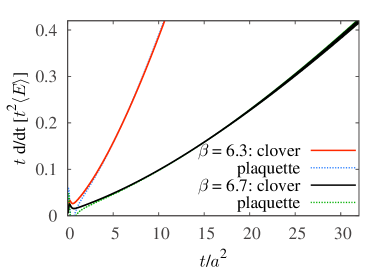
To illustrate the behaviors of $t^{2}\langle E(t)\rangle$ and $t\frac{d}{dt}t^{2}\langle E(t)\rangle$, we show these quantities with statistical errors as a function of $t/a^{2}$ in Fig. 1 for $\beta=6.3$ and $6.7$. To check the discretization effect on the operator, we compare $t^{2}\langle E(t)\rangle$ and $t\frac{d}{dt}t^{2}\langle E(t)\rangle$ defined from the clover-type representation with those defined from $E(t)=2(1-P(t))$ using the average plaquette $P(t)$ Luscher:2010iy . The figure shows that the difference between the two definitions is suppressed for large $t$. In particular, the difference is more suppressed in $t\frac{d}{dt}t^{2}\langle E(t)\rangle$ than that in $t^{2}\langle E(t)\rangle$, i.e., the discretization effect in the former is smaller than the latter. The figure also shows that both quantities increase monotonically as $t/a^{2}$ increases except for the small $t/a^{2}$ region where the lattice distortion effect is sizable. Furthermore, they show approximately linear behavior within the range $0.2\leq X\leq 0.4$. In Table 1, the values of $w_{{}_{X}}(a)$ and $t_{{}_{X}}(a)$ obtained from Eqs. (5) and (6) with $X=0.2$, $0.3$ and $0.4$ are given for each set of parameters. For simplicity, we will use the notations, $w_{{}_{X}}$ and $t_{{}_{X}}$, even for non-zero values of $a$. Note that the variances of $w_{{}_{X}}$ and $t_{{}_{X}}$ are approximately proportional to the inverse of physical volume of the lattice, while their dependence on $a$ should be small because gauge invariant operators at positive flow time is automatically renormalized Luscher:2010iy . The statistical error shown in Table 1 indeed shows such dependences on the spatial volume and lattice spacing.

Table 1: Simulation parameters $\beta$ and $N_{\rm s}$, and number of configurations, $N_{\mathrm{conf}}$. The result for the values of $w_{{}_{X}}/a$ and $\sqrt{t_{{}_{X}}}/a$ are also presented.

$\beta$	$N_{\rm s}$	$N_{\mathrm{conf}}$	$w_{0.4}/a$	$w_{0.3}/a$	$w_{0.2}/a$	$\sqrt{t_{0.4}}/a$	$\sqrt{t_{0.3}}/a$	$\sqrt{t_{0.2}}/a$	$N_{\rm s}a/w_{0.2}$
6.3	64	30	3.208(7)	2.877(5)	2.460(4)	3.269(4)	2.835(3)	2.254(2)	26.02	*
6.4	64	100	3.697(5)	3.317(4)	2.837(3)	3.765(3)	3.263(3)	2.590(2)	22.56	*
6.5	64	49	4.231(10)	3.797(8)	3.249(7)	4.310(8)	3.736(6)	2.965(4)	19.70	*
6.6	64	100	4.857(11)	4.356(9)	3.725(7)	4.938(8)	4.277(6)	3.390(4)	17.18	*
6.7	64	30	5.558(27)	4.980(23)	4.252(17)	5.638(20)	4.878(16)	3.863(10)	15.05	*
6.8	64	100	6.300(20)	5.652(17)	4.833(13)	6.406(16)	5.548(12)	4.395(08)	13.24	*
6.9	64	30	7.165(62)	6.431(52)	5.503(40)	7.289(47)	6.313(36)	5.000(23)	11.63	*
7.0	64	209	8.177(34)	7.322(28)	6.250(21)	8.287(25)	7.168(19)	5.674(12)	10.24
7.0	96	60	8.137(21)	7.297(18)	6.236(13)	8.264(16)	7.154(12)	5.665(08)	15.39	*
7.2	64	204	10.843(102)	9.646(80)	8.176(58)	10.833(69)	9.326(51)	7.343(31)	7.83
7.2	96	53	10.428(78)	9.348(66)	7.984(52)	10.586(62)	9.162(48)	7.256(31)	12.02	*
7.4	96	52			10.426(106)		11.927(98)	9.415(64)	9.21
7.4	128	40		12.084(61)	10.306(42)		11.808(40)	9.337(28)	12.42	*
7.5	128	60			11.706(72)			10.601(42)	10.94	*

Figure 1: $t^{2}\langle E(t)\rangle$ (the left panel) and $t\frac{d}{dt}t^{2}\langle E(t)\rangle$ (the right panel) as functions of $t/a^{2}$ for $\beta=6.3$ and $6.7$. Together with the result obtained with the clover-type operator for $E$, the one with $E$ defined from the plaquette is also presented for each parameter. The statistical error is smaller than the width of the lines.

III.2 Estimation of $w_{{}_{X}}$ for large $X$ in high $\beta$ region

Figure 2: Ratios $w_{0.4}/w_{0.2}$ and $\sqrt{t_{0.4}/t_{0.2}}$ as a function of the lattice spacing. Squares represent the results with the clover-type representation of $E$, while circles show those with plaquette one. Solid and dashed lines represent $8$-point and $9$-point linear fits and the extrapolated values to the continuum limit are shown at $a^{2}/w_{0.2}^{2}=0$ and $-0.005$, respectively.

As pointed out in Ref. Borsanyi:2012zs , the discretization error of $w_{0.3}$ is smaller than $t_{0.3}$, so that we employ $w_{{}_{X}}$ as the key reference scale in this paper. Note that the lattice artifact is expected to be smaller for larger $X$.

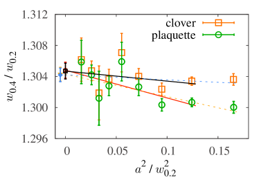
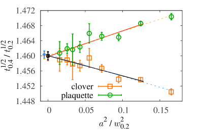
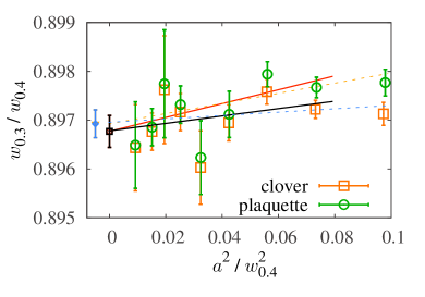
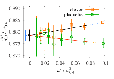
In our simulations, we estimate $w_{0.4}/a$ for $\beta=7.4$, $7.5$ using the data at small flow time ($w_{0.2}/a$) for these $\beta$ and the extrapolation of the ratio $w_{0.4}/w_{0.2}$ to the continuum limit. We plot $9$ data points for $w_{0.4}/w_{0.2}$ in the interval $6.3\leq\beta\leq 7.2$ as a function of $a^{2}/w_{0.2}^{2}$ in the left panel of Fig. 2. In the figure, the results are shown for clover- and plaquette-type representations of $E$. The error bars of the data points are estimated by the jackknife method for the ratios and not for the individuals. To take the continuum limit, we perform a linear fit with all $9$ points and that with $8$ points by removing the data for the coarsest lattice. The same procedure for the continuum extrapolations will be adopted throughout this paper. The values in the continuum limit obtained from Fig. 2 with the clover representation are $(w_{0.4}/w_{0.2})_{a\to 0}=1.3042(9)$ and $1.3047(10)$. The continuum extrapolation with the plaquette representation agrees well with this result. Similar extrapolation for $t_{{}_{X}}$ shown in the right panel of Fig. 2 leads to $(\sqrt{t_{0.4}/t_{0.2}})_{a\to 0}=1.4604(9)$ and $1.4600(11)$.

The left panel of Fig. 2 indicates that the lattice discretization error for the ratio $w_{0.4}/w_{0.2}$ is small. With this fact in mind, we estimate the values of $w_{0.4}/a$ at $\beta=7.4$ and $7.5$ using the numerical results of $w_{0.2}/a$ and the linear fit shown in Fig. 2 (left). The results are $w_{0.4}/a=13.445(55)(5)$ at $\beta=7.4$ and $w_{0.4}/a=15.272(95)(6)$ at $\beta=7.5$. The first error in the parenthesis is from the statistical error of $w_{0.2}/a$ and the fit parameters, while the second error is the systematic error obtained from the $9$-point linear fit. The latter is more than one order of magnitude smaller than the former.

III.3 Effect of the finite volume

In order to investigate the finite volume effect, we have performed the numerical analyses for two different values of $N_{\rm s}$ for $\beta=7.0$, $7.2$ and $7.4$ as shown in Table 1, where the spatial sizes in physical unit normalized by $w_{0.2}$, $L/w_{0.2}=N_{\rm s}a/w_{0.2}$, are shown for each set of configurations.

The comparison of the results with different $N_{\rm s}$ for $\beta=7.0$ and $7.4$ in Table 1 shows that the values of $w_{{}_{X}}/a$ and $\sqrt{t_{{}_{X}}}/a$ for different $N_{\rm s}$ agree within the statistics. On the other hand, the results for $\beta=7.2$ have statistically significant $N_{\rm s}$ dependence between $N_{\rm s}=64$ and $96$. These results suggest that the finite volume effect modifies the numerical results for $L/w_{0.2}=7.83$, while the effect is not visible for $L/w_{0.2}>9.21$ in the present statistics. This is the reason why we use the data sets with $*$ in the last column of Table 1.

III.4 Parametrization by the bare coupling $\beta$

For various practical applications, it is convenient to introduce a parametrization of the ratio $w_{0.4}/a$ in terms of $\beta$. We have carried out such parametrization using four types of fitting functions (polynomial type, one-loop type, Padé type, two-loop type) as summarized in Appendix A: All these fitting functions can reproduce the numerical results in Table. 1 well with three or four parameters. Among them, the three parameter fit motivated by the one-loop perturbation theory provides a reasonable result ($\chi^{2}/{\mathrm{dof}}=0.917$) for $11$ data points in $6.3\leq\beta\leq 7.5$ without over fitting:

$$\frac{w_{0.4}}{a}=\exp\left(\frac{4\pi^{2}}{33}\beta-8.6853+\frac{37.422}{\beta}-\frac{143.84}{\beta^{2}}\right)[1\pm 0.004(\mathrm{stat.})\pm 0.007(\mathrm{sys.})]$$ (7)

Figure 3: (Left) Result of the three parameter fit of $w_{0.4}/a$ given in Eq. (7). Squares are the data in Table 1 normalized by Eq. (7). Shaded band indicates the uncertainty originating from the errors of the fitted coefficients. Results with several other fitting functions normalized by Eq. (7) are also plotted as well; see, Appendix A. (Right) The same result is plotted for a wide range of $\beta$.

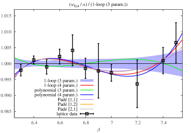
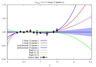
In the left panel of Fig. 3, we show the numerical results of Table 1 normalized by the fitting function Eq. (7). The shaded band in Fig. 3 is the error associated with the fitting parameters in Eq. (7). The results of some other fitting functions in Appendix A normalized by Eq. (7) are also plotted in Fig. 3. They agree with each other within $0.5\%$ in the range, $6.3\leq\beta\leq 7.5$. In the right panel of Fig. 3, the fitting functions are plotted in the region beyond the present $\beta$. Although the difference among the curves grows as $\beta$ becomes large, the deviation is still within $7\%$ even at $\beta=8.0$.

III.5 Continuum extrapolation of $w_{{}_{X}}$ and $t_{{}_{X}}$

We extract the continuum limits of $\sqrt{t_{{}_{X}}}/w_{0.4}$ and $w_{{}_{X}}/w_{0.4}$ with $X=0.2$, $0.3$ and $0.4$ by plotting those quantities as a function of $a^{2}/w_{0.4}^{2}$ and making linear extrapolation to $a=0$. Shown in Fig. 4 are two examples of such extrapolation for $X=0.3$. The resultant values are shown in Table 2, where the statistical error in the first parenthesis is estimated by $8$-point linear extrapolation, while the systematic error in the second parenthesis is obtained by the difference between the $8$-point and $9$-point analyses as mentioned earlier.

Figure 4: Continuum extrapolations of the ratios $\sqrt{t_{0.3}}/w_{0.4}$ and $w_{0.3}/w_{0.4}$. Squares represent the results with the clover-type representation of $E$, and circles are those with plaquette one.

$\sqrt{t_{0.4}}/w_{0.4}$	$\sqrt{t_{0.3}}/w_{0.4}$	$\sqrt{t_{0.2}}/w_{0.4}$	$w_{0.3}/w_{0.4}$	$w_{0.2}/w_{0.4}$
1.0164(32)(3)	0.8785(24)(0)	0.6952(18)(2)	0.8968(3)(2)	0.7665(6)(2)

Table 2: Continuum limits of $\sqrt{t_{{}_{X}}}/w_{0.4}$ and $w_{{}_{X}}/w_{0.4}$ for $X=0.2$, $0.3$ and $0.4$. The statistical and systematic errors are shown in the first and second parenthesis, respectively.

III.6 Relation to other reference scales

$r_{c}/w_{0.4}$	$r_{0}/w_{0.4}$	$\sqrt{\sigma}w_{0.4}$	$T_{c}w_{0.4}$	$w_{0.4}\Lambda_{\overline{\mathrm{MS}}}$
1.328(21)(7)	2.587(45)	0.455(8)	0.285(5)	0.233(19)

Table 3: Relations of $w_{0.4}$ with other reference scales in the continuum limit. For the details of the determination of these values and the estimate of the errors, see the text.

Figure 5: Continuum extrapolation of the ratio $r_{c}/w_{0.4}$ using $3$-point and $4$-point linear fits.

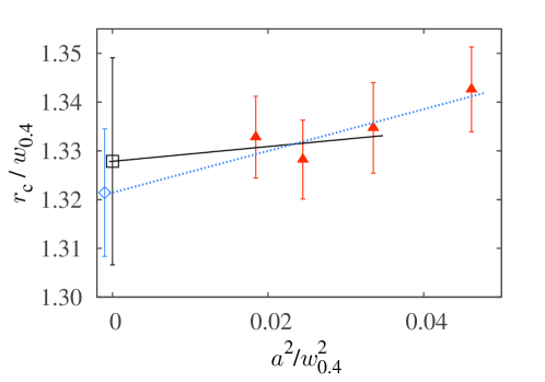
We now relate $w_{0.4}$ with other scales used in the literature. In Ref. Necco:2001xg , a scale $r_{c}$ determined from the force $F(r)$ between heavy quarks as $r_{c}^{2}F(r_{c})=0.65$ is introduced and $r_{c}/a$ was measured for four $\beta$ values in the range $6.57\leq\beta\leq 6.92$. Using Eq. (7), the result can be converted to the ratio $r_{c}/w_{0.4}$, which are plotted in Fig. 5. The continuum extrapolation $r_{c}/w_{0.4}|_{a\to 0}$ obtained from the figure is given in the first column of Table 3, where the error in the second parenthesis includes the systematic error from the linear fit and also the uncertainly from the fitting function in Eq. (7).

The relation between $w_{0.4}$ and the Sommer scale $r_{0}$ defined by $r_{0}^{2}F(r_{0})=1.65$ is also obtained by $r_{c}/r_{0}=0.5133(24)$ given in Ref. Necco:2001xg ; this is shown in the second column of Table 3, where the error takes into account all statistical and systematic ambiguities. The relation between $r_{0}$ and the string tension $\sqrt{\sigma}$ is studied in Ref. Edwards:1997xf with the result $r_{0}\sqrt{\sigma}=1.178$ within $1\%$ uncertainty. The resulting value of $\sqrt{\sigma}w_{0.4}$ is shown in the third column of Table 3. We note that the continuum-extrapolated value of $\sqrt{t_{0}}/r_{0}$ is estimated on coarser lattices in Refs. Luscher:2010iy ; Ce:2014sfa . These values are consistent with our results within statistical errors.

In Table 3, we also show the relations of $w_{0.4}$ with the critical temperature of the deconfinement transition $T_{c}$ and lambda parameter $\Lambda_{\overline{\mathrm{MS}}}$ in the $\overline{\mathrm{MS}}$ scheme, where we used $T_{c}/\sqrt{\sigma}=0.625\pm 0.003(+0.004)$ Boyd:1996bx and $r_{0}\Lambda_{\overline{\mathrm{MS}}}=0.602(48)$ Capitani:1998mq . We note that, in Ref. Boyd:1996bx , the value of $\beta$ corresponding to the critical temperature with $N_{\tau}=12$ is obtained as $\beta_{c}=6.3384$. This together with Eq. (7) leads to

$$T_{c}w_{0.4}=0.2826(3),$$ (8)

which is consistent with the value in Table 3.

We note that $\Lambda_{\overline{\mathrm{MS}}}$ can be also determined by matching the tadpole improved coupling constant to that in the ${\overline{\mathrm{MS}}}$-scheme Gockeler:2005rv . In Appendix B, we estimated the ratio $w_{0.4}\Lambda_{\overline{\mathrm{MS}}}$ by the same analysis as in Ref. Gockeler:2005rv using our numerical data on plaquette and $w_{0.4}/a$: The result reads

$$w_{0.4}\Lambda_{\overline{\mathrm{MS}}}=0.2388(5)(13),$$ (9)

which is consistent with the result in Table 3.

III.7 Relation to other parametrizations

Figure 6: Comparison of the fitting function Eq. (7) with previous results in Refs. Edwards:1997xf ; Guagnelli:1998ud ; Necco:2001xg ; Durr:2006ky . The numerical results on $w_{0.4}/a$ measured in the present study and $r_{c}/a$ and $r_{0}/a$ in Ref. Necco:2001xg are also plotted. $r_{c}/a$ and $r_{0}/a$ are converted to $w_{0.4}$-scale using the ratios in Table 3.

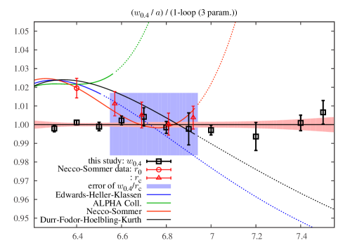
Let us compare our parametrization Eq. (7) with those introduced in previous studies; Edwards, Heller and Klassen ($5.6\leq\beta\leq 6.5$) Edwards:1997xf , Alpha Collaboration ($5.7\leq\beta\leq 6.57$) Guagnelli:1998ud , Necco and Sommer ($5.7\leq\beta\leq 6.92$) Necco:2001xg , and Dürr, Fodor, Hoelbling and Kurth ($5.7\leq\beta\leq 6.92$) Durr:2006ky . Each parametrization is based on the data obtained in the range of $\beta$ given in the parentheses. In Refs. Guagnelli:1998ud and Necco:2001xg , fitting functions of the polynomial form are used, while in Refs. Edwards:1997xf and Durr:2006ky the fitting functions motivated by the perturbative formula are employed.

In Fig. 6, we show the parametrizations of the above four references normalized by ours, Eq. (7). For the conversion among different reference scales, we have used the ratios in Table 3. The error of $r_{c}/w_{0.4}$, which dominates the ambiguity in the relations between $w_{0.4}$ and other scales, is also shown by the shaded box in the figure. The figure shows that the parametrizations in the previous studies agree with ours within this error band in the range of $\beta$, at which both fitting functions are reliable. The parametrizations in Refs. Guagnelli:1998ud and Necco:2001xg using polynomial ansätze have significant deviation from ours for $\beta$ outside the applicable range, while those of the parametrizations in Refs. Edwards:1997xf and Durr:2006ky are much milder at the level of $4-6\%$ for $\beta=7.5$.

In Fig. 6, the numerical results on $r_{0}/a$ and $r_{c}/a$ in Ref. Necco:2001xg converted to $w_{0.4}/a$ using the values in Table 3 are also presented. The error bars of these points are the statistical errors in Ref. Necco:2001xg , and do not include the ones associated with $r_{c}/w_{0.4}$ and $r_{0}/w_{0.4}$. The figure indicates that the $r_{0}/a$ and $r_{c}/a$ in Ref. Necco:2001xg systematically deviate from our results as $\beta$ becomes smaller. This may come from the discretization effect associated with the determination of $r_{0}$ on the lattice; these different parametrizations do not need to agree, because different determinations of the reference scales can differ by discretization effect. We also note that the statistical error in our numerical analysis of $w_{0.4}/a$ is significantly smaller than the previous ones for $6.4\lesssim\beta\lesssim 7.0$.

IV Summary

In this paper, we have performed an analysis of the flow time, $t$, dependence of $t^{2}\langle E(t)\rangle$ and its logarithmic derivative for SU(3) Yang–Mills theory with $6.3\leq\beta\leq 7.5$ in large lattice volumes $N_{\rm s}^{4}$ ($N_{\rm s}=64$–$128$). The results were utilized to parametrize the $\beta$ dependence of the lattice spacing, Eq. (7). In our analysis, the reference scale is chosen to be $w_{0.4}$, which is expected to suffer less discretization error than commonly used $w_{0.3}$ and $t_{0.3}$. The discretization and finite volume errors on our results are well suppressed with the present numerical settings.

After the completion of this paper, we found the paper Francis:2015lha in which $T_{c}\sqrt{t_{0.3}}=0.2489(14)$ in SU(3) Yang–Mills theory is obtained. This is consistent with $T_{c}\sqrt{t_{0.3}}=0.2483(7)$ obtained from the values in Table 2 and Eq. (8).

Appendix A Fit functions

In this appendix, we show the four fit functions we employed to parametrize $w_{0.4}/a$ in terms of $\beta$:

1. Polynomials of $\beta-\beta_{0}$:

   $$\log\left(\frac{w_{0.4}}{a}\right)_{\mathrm{poly}}(\beta)=a_{0}+a_{1}(\beta-\beta_{0})+a_{2}(\beta-\beta_{0})^{2}+a_{3}(\beta-\beta_{0})^{3}.$$ (10)

2. One-loop perturbation + polynomials of $1/\beta$:

   $$\log\left(\frac{w_{0.4}}{a}\right)_{\text{1-loop}}(\beta)=\frac{4\pi^{2}}{33}\beta+c_{0}+\frac{c_{1}}{\beta}+\frac{c_{2}}{\beta^{2}}+\frac{c_{3}}{\beta^{3}}+\cdots.$$ (11)

3. One-loop perturbation + Padé improved polynomials of $1/\beta$ :

   $$\log\left(\frac{w_{0.4}}{a}\right)_{\text{Pad\'{e}}}(\beta)=\frac{4\pi^{2}}{33}\beta+d_{0}\frac{1+d_{1}/\beta+d_{2}/\beta^{2}}{1+e_{1}/\beta+e_{2}/\beta^{2}}.$$ (12)

4. Two-loop perturbation + polynomials of $1/\beta$:

   $$\log\left(\frac{w_{0.4}}{a}\right)_{\text{2-loop}}(\beta)=\frac{4\pi^{2}}{33}\beta-\frac{51}{121}\ln\beta+c^{\prime}_{0}+\frac{c^{\prime}_{1}}{\beta}+\frac{c^{\prime}_{2}}{\beta^{2}}+\cdots.$$ (13)

Here, $a_{i}$, $c_{i}$, $d_{i}$, $e_{i}$ and $c^{\prime}_{i}$ are fitting parameters. The polynomial form Eq. (10) is the one used in Refs. Necco:2001xg and Guagnelli:1998ud . In the three-parameter fit with Eqs. (10), (11) and (13), we set $a_{3}$, $c_{3}$ and $c^{\prime}_{3}$ to zero, respectively. In the fit with Eq. (12), we tried three parameter fit with $d_{2}=e_{2}=0$, four parameter fits with $e_{2}=0$ and $d_{2}=0$. We refer each fit to as [1,1], [2,1] and [1,2], respectively.

fit func.	$\chi^{2}$/dof
polynomial (3 param.)	1.496
polynomial (4 param.)	0.336
1-loop (3 param.)	0.917
1-loop (4 param.)	0.363
$[1,1]$ Padé (3 param.)	0.377
$[2,1]$ Padé (4 param.)	0.424
$[1,2]$ Padé (4 param.)	0.424

Table 4: Result of $\chi^{2}/{\mathrm{dof}}$ of the fits for $w_{0.4}/a$ with various fitting functions Eqs. (10)–(12).

In Table 4 we show $\chi^{2}/{\mathrm{dof}}$ for each fit functions. For the polynomial fit, Eq. (10), we take $\beta_{0}=7.0$; the quality of the fit with other choices of $\beta_{0}$ hardly changes. In the text, we employ the three parameter fit with Eq. (11) to obtain Eq. (7), since it provide reasonable $\chi^{2}/{\mathrm{dof}}\simeq 1$ without over fitting.

Appendix B Determination of $\Lambda$-parameter

In this appendix, we show the derivation of Eq.(9). In Ref. Gockeler:2005rv , $r_{0}\Lambda_{\overline{\mathrm{MS}}}$ is analyzed with the data of $r_{0}/a$ in Ref. Necco:2001xg . Here we adopt the same procedure by using the numerical results of $w_{0.4}/a$ and the average plaquette obtained in this study. Such an analysis allows us to determine the ratio $w_{0.4}\Lambda_{\overline{\mathrm{MS}}}$ directly using the accurate data on fine lattices.

The dimensionless parameter $a\Lambda_{\overline{\mathrm{MS}}}$ can be obtained by matching the tadpole improved lattice perturbation theory. The boosted coupling constant $g_{\square}$ is defined by

$$g_{\square}^{2}\equiv g_{0}^{2}(a)/u_{0}^{4},$$ (14)

where $u_{0}^{4}\equiv P=\langle\mathrm{Tr}\ U_{\square}\rangle/3$.

As for the choice of the renormalization scale and the running coupling constant, we take the following two methods:

• Method I

  $$a\Lambda_{\overline{\mathrm{MS}}}=a\mu_{\ast}F^{\overline{\mathrm{MS}}}(g_{\overline{\mathrm{MS}}}(\mu_{\ast}))$$ (15)

  at the scale

  $$a\mu_{\ast}=\exp\left(\frac{t_{1}^{\square}}{2b_{0}}\right),$$ (16)

  and

  $$\frac{1}{g_{\overline{\mathrm{MS}}}^{2}(\mu_{\ast})}=\frac{1}{g_{\square}^{2}(a)}+\left(\frac{b_{1}}{b_{0}}t_{1}^{\square}-t_{2}^{\square}\right)g_{\square}^{2}(a)+O(g_{\square}^{4}).$$ (17)

• Method II

  $$a\Lambda_{\overline{\mathrm{MS}}}=a\Lambda_{\square}\exp\left(\frac{t_{1}^{\square}}{2b_{0}}\right),$$ (18)

  with

  $$a\Lambda_{\square}=F^{\square}(g_{\square}(a)).$$ (19)

  This scheme corresponds to choosing a scale at

  $$a\mu_{=}=\exp\left(\frac{t_{1}^{\square}}{2b_{0}}\right)\frac{F^{\square}(g_{\square}(a))}{F^{\overline{\mathrm{MS}}}(g_{\square}(a)}$$ (20)

  in Method I.

In the $3$-loop order, $F^{S}$ ($S=\square$, $\overline{\mathrm{MS}}$) is expressed as

$$\frac{\Lambda^{S}}{M} \equiv F^{S}(g_{S}(M))=\exp\left(-\frac{1}{2b_{0}g_{S}^{2}}\right)(b_{0}g_{S}^{2})^{-\frac{b_{1}}{2b_{0}}}$$

$$\qquad{}\times\left(1+\frac{b_{1}+\sqrt{b_{1}^{2}-4b_{0}b_{s}^{S}}}{2b_{0}}g_{S}^{2}\right)^{-p_{A}^{S}}\left(1+\frac{b_{1}+\sqrt{b_{1}^{2}+4b_{0}b_{s}^{S}}}{2b_{0}}g_{S}^{2}\right)^{-p_{B}^{S}},$$ (21)

where

$$p_{A}^{S}=-\frac{b_{1}}{4b_{0}^{2}}-\frac{b_{1}^{2}-2b_{0}b_{2}^{S}}{4b_{0}^{2}\sqrt{b_{1}^{2}-4b_{0}b_{2}^{S}}},\qquad p_{B}^{S}=-\frac{b_{1}}{4b_{0}^{2}}+\frac{b_{1}^{2}-2b_{0}b_{2}^{S}}{4b_{0}^{2}\sqrt{b_{1}^{2}-4b_{0}b_{2}^{S}}}.$$ (22)

In the $[1,1]$ Padé approximation, it leads

$$F_{[1,1]}^{S}(g_{S}(M))=\exp\left(-\frac{1}{2b_{0}g_{S}^{2}}\right)\left[\frac{b_{0}g_{S}^{2}}{1+\left(\frac{b_{1}}{b_{0}}-\frac{b_{2}^{S}}{b_{1}}\right)g_{S}^{2}}\right]^{-\frac{b_{1}}{2b_{0}}}.$$ (23)

In SU(3) Yang–Mills theory, the coefficients are given by

$$b_{0}=\frac{11}{(4\pi)^{2}},\qquad b_{1}=\frac{102}{(4\pi)^{4}},\qquad b_{2}^{\overline{\mathrm{MS}}}=\frac{1}{(4\pi)^{6}}\frac{2857}{2},\qquad b_{2}^{\square}=b_{2}^{\overline{\mathrm{MS}}}+b_{1}t_{1}^{\square}-b_{0}t_{2}^{\square},$$ (24)

with

$$t_{1}^{\square}=0.1348680,\qquad t_{2}^{\square}=0.0217565.$$ (25)

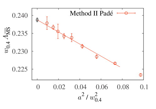
We adopt Method II with Padé improvement to estimate the central value of $w_{0.4}\Lambda_{\overline{\mathrm{MS}}}$, and use the results of Methods I and II without Padé improvement to estimate the systematic error. The results are summarized in Table 5: The values in the continuum limit are obtained by a linear fit as a function of $a^{2}/w_{0.4}^{2}$ without the coarsest lattice data (see Fig. 7). Then we find

$$w_{0.4}\Lambda_{\overline{\mathrm{MS}}}=0.2388(5)(13)$$ (26)

with the statistical and systematic errors.

$\beta$	$N_{\rm s}$	plaquette	$w_{0.4}/a$	$w_{0.4}\Lambda_{\overline{\mathrm{MS}}}$
				Method I	Method II	Method II Padé
6.3	64	0.622 420 85(30)	3.208( 7)	0.2248(4)	0.2253(4)	0.2234(4)
6.4	64	0.630 632 88(13)	3.697( 5)	0.2280(3)	0.2285(3)	0.2266(3)
6.5	64	0.638 361 33(35)	4.231(10)	0.2298(5)	0.2302(5)	0.2285(5)
6.6	64	0.645 669 58(12)	4.857(11)	0.2327(5)	0.2331(5)	0.2314(5)
6.7	64	0.652 608 39(39)	5.558(27)	0.2351(11)	0.2354(11)	0.2338(11)
6.8	64	0.659 215 11(11)	6.300(20)	0.2354(7)	0.2358(8)	0.2342(7)
6.9	64	0.665 522 54(33)	7.165(62)	0.2367(20)	0.2370(20)	0.2355(20)
7.0	96	0.671 556 729(89)	8.137(21)	0.2378(6)	0.2381(6)	0.2367(6)
7.2	96	0.682 891 86(22)	10.428(78)	0.2389(18)	0.2392(18)	0.2379(18)
$\infty$		1	$\infty$	0.2399(5)	0.2401(5)	0.2388(5)

Table 5: Simulation parameters $\beta$ and $N_{\rm s}$. The plaquette value, $w_{0.4}/a$, and $w_{0.4}\Lambda_{\overline{\mathrm{MS}}}$ using Method I, II and II with Padé approximation. The last row corresponds to the values at the continuum limit obtained from linear extrapolation without using the coarsest lattice data at $\beta=6.3$ (the italic number).

Figure 7: Values of $w_{0.4}\Lambda_{\overline{\mathrm{MS}}}$ estimated by the Method II with Padé improvement. The continuum limit is shown at $a^{2}/w_{0.4}^{2}=0$.

References

- (1) R. G. Edwards, U. M. Heller and T. R. Klassen, Nucl. Phys. B 517, 377 (1998) [hep-lat/9711003].
- (2) R. Sommer, Nucl. Phys. B 411, 839 (1994) [hep-lat/9310022].
- (3) M. Lüscher, Commun. Math. Phys. 293, 899 (2010) [arXiv:0907.5491 [hep-lat]].
- (4) M. Lüscher, JHEP 1008, 071 (2010) [arXiv:1006.4518 [hep-lat]].
- (5) S. Borsanyi, S. Dürr, Z. Fodor, C. Hoelbling, S. D. Katz, S. Krieg, T. Kurth and L. Lellouch et al., JHEP 1209, 010 (2012) [arXiv:1203.4469 [hep-lat]].
- (6) M. Lüscher and P. Weisz, JHEP 1102, 051 (2011) [arXiv:1101.0963 [hep-th]].
- (7) Z. Fodor, K. Holland, J. Kuti, D. Nogradi and C. H. Wong, JHEP 1211, 007 (2012) [arXiv:1208.1051 [hep-lat]].
- (8) P. Fritzsch and A. Ramos, JHEP 1310, 008 (2013) [arXiv:1301.4388 [hep-lat]].
- (9) M. Lüscher, JHEP 1304, 123 (2013) [arXiv:1302.5246 [hep-lat]].
- (10) M. Lüscher, PoS LATTICE 2013, 016 (2014) [arXiv:1308.5598 [hep-lat]].
- (11) Z. Fodor, K. Holland, J. Kuti, S. Mondal, D. Nogradi and C. H. Wong, JHEP 1409, 018 (2014) [arXiv:1406.0827 [hep-lat]].
- (12) K. Kikuchi and T. Onogi, JHEP 1411, 094 (2014) [arXiv:1408.2185 [hep-th]].
- (13) A. Hasenfratz, D. Schaich and A. Veernala, arXiv:1410.5886 [hep-lat].
- (14) A. Ramos and S. Sint, arXiv:1411.6706 [hep-lat].
- (15) S. Aoki, K. Kikuchi and T. Onogi, arXiv:1412.8249 [hep-th].
- (16) C. Monahan and K. Orginos, arXiv:1501.05348 [hep-lat].
- (17) H. Suzuki, PTEP 2013, no. 8, 083B03 (2013) [arXiv:1304.0533 [hep-lat]].
- (18) L. Del Debbio, A. Patella and A. Rago, JHEP 1311, 212 (2013) [arXiv:1306.1173 [hep-th]].
- (19) H. Makino and H. Suzuki, PTEP 2014, no. 6, 063B02 (2014) [arXiv:1403.4772 [hep-lat]].
- (20) H. Makino and H. Suzuki, PTEP 2015, no. 3, 033B08 [arXiv:1410.7538 [hep-lat]].
- (21) H. Makino, F. Sugino and H. Suzuki, PTEP 2015, no. 4, 043B07 [arXiv:1412.8218 [hep-lat]].
- (22) H. Suzuki, PTEP 2015, no. 4, 043B04 [arXiv:1501.04371 [hep-lat]].
- (23) M. Asakawa et al. [FlowQCD Collaboration], Phys. Rev. D 90, 011501 (2014) [arXiv:1312.7492 [hep-lat]].
- (24) M. Kitazawa, M. Asakawa, T. Hatsuda, T. Iritani, E. Itou and H. Suzuki, arXiv:1412.4508 [hep-lat].
- (25) M. Guagnelli et al. [ALPHA Collaboration], Nucl. Phys. B 535, 389 (1998) [hep-lat/9806005].
- (26) S. Necco and R. Sommer, Nucl. Phys. B 622, 328 (2002) [hep-lat/0108008].
- (27) M. Cè, C. Consonni, G. P. Engel and L. Giusti, PoS LATTICE 2014, 353 (2014) [arXiv:1410.8358 [hep-lat]].
- (28) G. Boyd, J. Engels, F. Karsch, E. Laermann, C. Legeland, M. Lütgemeier and B. Petersson, Nucl. Phys. B 469, 419 (1996) [hep-lat/9602007].
- (29) S. Capitani et al. [ALPHA Collaboration], Nucl. Phys. B 544, 669 (1999) [hep-lat/9810063].
- (30) M. Göckeler, R. Horsley, A. C. Irving, D. Pleiter, P. E. L. Rakow, G. Schierholz and H. Stüben, Phys. Rev. D 73, 014513 (2006) [hep-ph/0502212].
- (31) S. Dürr, Z. Fodor, C. Hoelbling and T. Kurth, JHEP 0704, 055 (2007) [hep-lat/0612021].
- (32) A. Francis, O. Kaczmarek, M. Laine, T. Neuhaus and H. Ohno, arXiv:1503.05652 [hep-lat].