Optimizing User Association and Activation Fractions in Heterogeneous Wireless Networks

Vaibhav Singh, Narayan Prasad, Mustafa Arslan, Sampath Rangarajan e-mail: vaibhavs@umd.edu, {prasad, marslan, sampath}@nec-labs.com
Abstract

We consider the problem of maximizing the alpha-fairness utility over the downlink of a heterogeneous wireless network (HetNet) by jointly optimizing the association of users to transmission points (TPs) and the activation fractions of all TPs. Activation fraction of each TP is the fraction of the frame duration for which it is active, and together these fractions influence the interference seen in the network. To address this joint optimization problem we adopt an approach wherein the activation fractions and the user associations are optimized in an alternating manner. The sub-problem of determining the optimal activation fractions is solved using an auxiliary function method that we show is provably convergent and is amenable to distributed implementation. On the other hand, the sub-problem of determining the user association is solved via a simple combinatorial algorithm. Meaningful performance guarantees are derived and a distributed variant offering identical guarantees is also proposed. The significant benefits of using the proposed algorithms are then demonstrated via realistic simulations.

I Introduction

It is well established by now that future cellular networks will be dense HetNets formed by a multitude of disparate transmission points deployed in a highly irregular fashion [1]. In a majority of these deployments, the transmission points (TPs) will be connected to each other by a non-ideal backhaul with a relatively high latency (several dozens of milliseconds). An unfortunate consequence of such a high latency is that it renders unsuitable resource management (RM) schemes that strive to coordinate and obtain allocation decisions within a fine time-scale (e.g., 1 ms in LTE HetNets) [2, 3, 4, 5, 6, 7]. Instead, semi-static resource management schemes where RM is performed at two time scales, are better suited since they are more robust towards backhaul latency. Broadly speaking, in any such semi-static scheme the RM that is done at a coarse frame level granularity (that is at-least as large as the backhaul latency) entails coordination among TPs based on averaged (not instantaneous) slowly varying metrics. On the other hand, the RM in such a scheme that is done at a much finer slot level granularity involves no coordination among TPs and is done independently by each active TP based on fast changing metrics [8, 9, 10, 11, 12]. The semi-static scheme that we propose in this paper decides at the onset of each frame which set of users should each TP serve over that frame such that each user is served by exactly one TP (user association) and how often should each TP transmit over that frame (activation fraction of that TP).

The problem at hand is quite challenging due to the well recognized interference coupling problem. Indeed, while increasing the activation fraction (AF) of a TP will help it serve more users (or serve a given set of users better), it injects more interference to all users being served by other TPs. User Association (without AF optimization) is by itself a popular HetNet RM scheme, wherein the interference coupling problem is simplified by assuming that the interference that would be seen by any user upon being associated to any TP remains static. Association is then determined by optimizing a system utility [13, 14, 15, 16, 17], or by minimizing a cost function given traffic demands [9], or by adopting a game theoretic framework [18]. Joint optimization of user association along with other system resources, such as power and bandwidth in the downlink [10, 11, 6, 12, 19] and user powers and TP locations in the uplink [20, 21], has also received significant attention. Considering the downlink which is our focus in this paper, we see that the alternating optimization framework is a popular approach to ensure tractability, and that binary (on-off) power control has been found to be particularly effective in terms of being robust and capturing most of the available gains with a small signalling footprint. The latter observation has led to another promising downlink semi-static RM technique that is fully compliant with the LTE standard, and seeks to capture the benefits of slot-level coordinated binary power control over a HetNet with a non ideal backhaul. This scheme combines user association with partial muting of the high power Macro TP, i.e., the Macro TP is allowed to be active (or transmit with a pre-determined power) for any fraction of the total number of slots in a frame. The choice of this AF for the macro TP is optimized together with the user association [22, 23]. The macro TP then adopts a muting pattern (which includes its on-off status on all the slots) conforming to the determined AF. Notice that the exact on-off status of the macro TP on all the slots is not optimized. Indeed, doing so can be detrimental since coordination done at a coarse time-scale based on the available averaged metrics cannot adapt to the fast changing channel and interference conditions seen across the slots.

Recent studies have shown that topologies without one common dominant interferer will be ubiquitous and in such cases optimizing the AF of only one TP is not enough. The problem we seek to solve is geared exactly towards such deployments. One attempt to solve our problem would be to extend the solutions proposed for the aforementioned scheme, but then it becomes immediately clear that those solutions do not scale when activation fractions for all TPs have to be optimized. This is because those solutions explicitly maintain a rate for each TP-user link under each possible interference pattern, which grow exponentially in the number of TPs. In this paper, we propose a simple formulation that imposes activation fractions and yields one average rate expression for each TP-user link. The latter expression is conservative and is a closed-form function of all activation fractions. Interestingly, in the absence of fast fading our rate expression reduces to the approximate rate expression introduced in [24] (see also [25]), which considered the problem of determining activation fractions to meet a given set of user traffic demands for a given user association. We confirm the observation made in those works that the rate expression is in-fact quite accurate over practical HetNets. Our main contributions are as follows:

  • We adopt $\alpha-$fairness utility as the system wide utility which generalizes all popular utility functions [26], wherein we also allow for assigning any arbitrary set of weights (reflecting priorities) to the users. We develop centralized and distributed algorithms that yield good solutions for any given fairness parameter $\alpha$. These algorithms are obtained by adopting an alternating optimization based approach. The latter approach is well justified since the problem at hand is intractable and our goal is to obtain unified low-complexity algorithms that are suitable for all $\alpha$.

  • For the discrete user-association sub-problem, we first prove that this sub-problem itself is NP-hard and proceed to completely characterize the underlying set function that needs to be optimized. We then suggest and comprehensively analyze a simple centralized combinatorial algorithm (referred to as the GLS algorithm) that involves a Greedy stage followed by Local Search improvements. Our analysis yields meaningful and novel readily computable performance guarantees for all $\alpha$. Previous related works have considered the proportional fairness (PF) utility and proposed combinatorial user association algorithms [15, 12]. Our results when specialized to the case of the weighted PF utility (by setting $\alpha=1$) reveal that GLS is optimal up-to a constant additive factor of $-2\ln(2)$. Thus, a simple algorithm yields optimality up-to an additive constant factor, a fact that was hitherto only established for a significantly more complex algorithm [15] (whose run-time can depend on the input weights). Upon further specializing to the case with identical user weights, we see that the guarantee proved for a greedy algorithm in [12] has an instance dependent (non constant) additive factor. Interestingly, our simulation results indicate that in this special case the association yielded by GLS is identical to the optimal one obtained via another more complex algorithm from [12].

  • We derive a distributed version of the GLS algorithm and prove that remarkably it provides guarantees identical to its centralized counterpart. This distributed version requires network assistance in the form of periodic broadcast of system load information similar to that proposed earlier in [27]. The main novelty of our approach is that we are able to configure each user to consider the system utility gain in contrast to the selfish gain used in the user-centric approach adopted by [27, 18] and more recently in [17]. Consequently, we can establish guarantees (with respect to the optimal system utility) and provable convergence for our distributed algorithms for all $\alpha$. We note here that convergence of the user-centric approach to a Nash equilibrium was proved in [18] for particular choices of $\alpha$ and the recent and independent work in [17] has identified conditions under which the Nash equilibrium is (near-)optimal.

  • For the continuous AF optimization sub-problem we adopt the auxiliary function method and show that it is provably convergent. Such a method has been used for precoder optimization originally over the single-cell downlink in [28] and over the multi-cell downlink in [7] followed by [11, 6]. We note however that unlike those works we incorporate fading coefficients that change at two different time scales. Further, a key step in our case entails a novel GP formulation, which we show can also be implemented in a distributed manner.

  • Finally, the performance of all our algorithms is compared to appropriate baselines via extensive simulations over a HetNet topology generated as per 3GPP LTE guidelines. Our results highlight the significant gains that can be achieved in realistic HetNet deployments via the joint optimization.

II Problem Statement

Considering the downlink in a HetNet, let ${\mathcal{U}}=\{1,\cdots,K\}$ denote the set of users and let ${\mathcal{B}}$ denote the set of transmission points (TPs) with cardinality $|{\mathcal{B}}|=B$. Further, suppose that the time axis is divided into multiple frames, where each frame consists of several consecutive slots. The fast fading coefficients for each user are assumed to change across slots in an independent identically distributed (i.i.d.) manner, while the slow fading coefficients are assumed to change across frames in an i.i.d. manner. The choice of the activation fraction for each TP along with the user association for all TPs is made once for each frame to optimize the system utility. This choice can be based on the slow fading realization in that frame but does not consider any previous such choices. Each TP then independently implements its per-slot scheduling policy over the users associated with it in that frame, where the latter scheduling policy respects the assigned activation fraction and can exploit the instantaneous fast fading coefficients seen by the associated users on each slot. Consequently, we can suppress the dependence on the frame and slot indices in the following.

In order to formulate an optimization problem for determining the user association and activation fractions, we derive an average rate that each user can obtain over a frame of interest, under any given user association and activation fractions. Towards this end, let ${\mathcal{U}}^{(b)},\;\forall b\in{\mathcal{B}}$ denote any given set of users associated to TP $b$ over the frame and let ${\bm{\rho}}=[\rho_{b}]_{b\in{\mathcal{B}}}$ denote the activation vector, where $\rho_{b}\in[0,1]$ denotes the activation fraction assigned to TP $b$. We proceed by assuming that each TP $b$ allocates a fraction $\gamma_{k,b}\in[0,1]$ of the frame to serve each associated user $k\in{\mathcal{U}}^{(b)}$, such that $\sum_{k\in{\mathcal{U}}^{(b)}}\gamma_{k,b}=1$, where these fractions are determined at the onset of the frame. In particular, each TP is assumed to adopt an optimal fractional round robin per-slot scheduling policy. Note that an efficient per-slot scheduling policy (cf. [29]) that can adapt to the instantaneous fading and interference conditions seen across all the slots, will be at-least as good (in terms of optimizing the given utility). Next, we assume that the activation fraction of each TP $b$ is implemented via a Bernoulli random variable ${\mathcal{X}}_{b}$ with $E[{\mathcal{X}}_{b}]=\rho_{b}$, that is i.i.d. across slots in the frame and is independent of all other random variables. Specifically, TP $b$ is assumed to transmit (with a fixed power) when ${\mathcal{X}}_{b}=1$ and remain silent otherwise. Then, an average rate that can be achieved for user $k\in{\mathcal{U}}^{(b)}$ is given by,

$\displaystyle\gamma_{k,b}\rho_{b}\mathbb{E}\left[\log\left(1+\frac{\beta_{k,b}}{1+\sum_{b^{\prime}\neq b}{\beta_{k,b^{\prime}}{\mathcal{X}}_{b^{\prime}}}}\right)\right]$ (1)

where the the desired channel gain $\beta_{k,b}$ and the interfering channel gains $\{\beta_{k,b^{\prime}}\}$ are random variables that include both fast and slow fading as well as noise normalized transmit powers, and the expectation is over the activation variables as well as the fast fading. Upon invoking the fact that the instantaneous rate in (1) is convex in the activation variables, which we recall are independent of the fast fading coefficients, we can further lower bound (1) to obtain

$\displaystyle r_{k}=\gamma_{k,b}\underbrace{\rho_{b}\mathbb{E}\left[\log\left(1+\frac{\beta_{k,b}}{1+\sum_{b^{\prime}\neq b}{\beta_{k,b^{\prime}}\rho_{b^{\prime}}}}\right)\right]}_{\stackrel{{\scriptstyle\scriptscriptstyle\triangle}}{{=}}R_{k,b}({\bm{\rho}})},$ (2)

where now the expectation is over only the fast fading. Note that $r_{k}$ in (2) depends on the slow fading realization (comprising of the path losses and shadowing factors) over the frame of interest. Letting ${{\mathbf{r}}}=[r_{1},\cdots,r_{K}]$ denote the vector of such conservative rates obtained for all the $K$ users over the frame, the achieved system utility is given by

$\displaystyle\sum_{k\in{\mathcal{U}}}w_{k}u(r_{k},\alpha),$ (3)

where $\alpha>0$ is a tunable fairness parameter and

$\displaystyle u(r_{k},\alpha)=\left\{\begin{array}[]{rl}\frac{r_{k}^{(1-\alpha)}}{1-\alpha}&\;\;\;\;\;\;\alpha\in(0,1)\\ \log(r_{k})&\;\;\;\;\;\;\;\;\alpha=1\\ -\frac{r_{k}^{(1-\alpha)}}{\alpha-1}&\;\;\;\;\;\;\alpha>1\end{array}\right.$ (7)

and $w_{k}>0$ denotes the weight of user $k\in{\mathcal{U}}$. These weights can be used to assign different priorities to different users and we assume that they are normalized, i.e., $\sum_{k\in{\mathcal{U}}}w_{k}=1$. We can now write our problem, which is a mixed optimization problem, as

$$\boxed{\begin{aligned} \max_{{\bm{\rho}}\in[0,1]^{B};x_{k,b}\in\{0,1\};\atop\gamma_{k,b}\in[0,1]\;\forall\;k,b}\left\{\sum_{k\in{\mathcal{U}}}\sum_{b\in{\mathcal{B}}}x_{k,b}\left(w_{k}u(\gamma_{k,b}R_{k,b}({\bm{\rho}}))\right)\right\}\\ {\rm s.t.}\sum_{b\in{\mathcal{B}}}x_{k,b}=1,\;\forall\;k\in{\mathcal{U}};\;\sum_{k\in{\mathcal{U}}}\gamma_{k,b}=1\;\forall\;b\in{\mathcal{B}}.\end{aligned}}$$ (8)

Note that in (8) the binary variable $x_{k,b}$ is one if user $k$ is associated to TP $b$ and zero otherwise, so that the first set of constraints ensures that each user is associated with only one TP. Consequently, ${\mathcal{U}}^{(b)}\stackrel{{\scriptstyle\scriptscriptstyle\triangle}}{{=}}\{k:x_{k,b}=1\}_{k\in{\mathcal{U}}}$ yields the user set associated with TP $b$. Note that in (8), we enforce $\{{\mathcal{U}}^{(b)}\}_{b\in{\mathcal{B}}}$ to be a partition of ${\mathcal{U}}$. This is meaningful and indeed important since we are targeting short-term optimality by maximizing a system utility independently over each frame. The joint optimization problem in (8) is unfortunately intractable. Consequently, we develop an alternating optimization framework to solve the joint problem in (8). We will demonstrate that although the user association and activation fractions are optimized assuming conservative rates and optimal fractional round robin per-slot scheduling policies at all TPs, the obtained solution retains its significant gains even without these assumptions. To improve readability the proofs of all the following propositions are deferred to the appendix.

III User Association

We adopt the convention that $0\ln(0)=0$ and consider any fixed activation vector ${\bm{\rho}}$ with strictly positive elements (otherwise any TP $b$ with $\rho_{b}=0$ can be simply removed). We proceed to systematically consider the user-association sub-problem of (8) given by

$$\begin{split}&\mbox{max}_{x_{k,b}\in\{0,1\};\atop\gamma_{k,b}\in[0,1]\;\forall\;k,b}\left\{\sum_{k\in{\mathcal{U}}}\sum_{b\in{\mathcal{B}}}x_{k,b}\left(w_{k}u(\gamma_{k,b}R_{k,b}({\bm{\rho}}))\right)\right\}\\ &{\rm s.t.}\sum_{b\in{\mathcal{B}}}x_{k,b}=1,\;\forall\;k\in{\mathcal{U}};\;\sum_{k\in{\mathcal{U}}}\gamma_{k,b}=1\;\forall\;b\in{\mathcal{B}},\end{split}$$ (9)

over three regimes defined by the values of $\alpha$. We first define a ground set, ${\underline{\Omega}}=\{(k,b):k\in{\mathcal{U}},b\in{\mathcal{B}}\}$, that consists of all possible tuples and where each tuple $(k,b)$ denotes an association of user $k$ to TP $b$. Then, we also define the set ${\underline{\Omega}}^{(b)}=\{(k,b):k\in{\mathcal{U}}\}$ for each TP $b\in{\mathcal{B}}$ which consists of all tuples whose TP is $b$, along with the set ${\underline{\Omega}}_{(k)}=\{(k,b):b\in{\mathcal{B}}\}$ for each user $k$ which consists of all tuples whose user is $k$. Finally, we define a family of sets ${\underline{{\bm{\mathcal{I}}}}}$, as the one which includes each subset of ${\underline{\Omega}}$ such that the tuples in that subset have mutually distinct users. Formally,

$\displaystyle{\underline{\mathcal{G}}}\subseteq{\underline{\Omega}}:|{\underline{\mathcal{G}}}\cap{\underline{\Omega}}_{(k)}|\leq 1\;\forall\;k\Leftrightarrow{\underline{\mathcal{G}}}\in{\underline{{\bm{\mathcal{I}}}}}.$ (10)

We start with the regime $\alpha>1$ and note that for any given user association, i.e, for any given feasible choice of variables $\{x_{k,b}\}$, (LABEL:eq:Bigoriginal) is a continuous optimization problem. Moreover, it is separable across the set of TPs and for each TP $b\in{\mathcal{B}}$, we have a convex optimization problem over the set of variables $\{\gamma_{k,b}\}$ for $k\in{\mathcal{U}}:x_{k,b}=1$. Using K.K.T. conditions it is verified in the appendix that for each TP $b\in{\mathcal{B}}$

$\displaystyle\begin{split}&\mbox{max}_{\gamma_{k,b}\in[0,1]\;\forall\;k\atop\sum_{k\in{\mathcal{U}}}\gamma_{k,b}=1}\left\{\sum_{k\in{\mathcal{U}}}x_{k,b}\left(w_{k}u(\gamma_{k,b}R_{k,b}({\bm{\rho}}))\right)\right\}=\\ &-\left(\sum_{k\in{\mathcal{U}}}x_{k,b}\left(w_{k}\frac{(R_{k,b}({\bm{\rho}}))^{1-\alpha}}{\alpha-1}\right)^{1/\alpha}\right)^{\alpha}\end{split}$ (11)

Consequently, upon defining

$\displaystyle\begin{split}&\Theta_{k}^{(b)}(\alpha)=\left(w_{k}\frac{(R_{k,b}({\bm{\rho}}))^{1-\alpha}}{\alpha-1}\right)^{1/\alpha},\;\forall\;\alpha>1,\end{split}$

(LABEL:eq:Bigoriginal) reduces to the following discrete optimization problem.

$\displaystyle\begin{split}&\mbox{min}_{x_{k,b}\in\{0,1\}\;\forall\;k,b\atop\sum_{b\in{\mathcal{B}}}x_{k,b}=1\;\forall\;k}\left\{\sum_{b\in{\mathcal{B}}}\left(\sum_{k\in{\mathcal{U}}}x_{k,b}\Theta_{k}^{(b)}(\alpha)\right)^{\alpha}\right\}.\end{split}$ (12)

Considering the case $\alpha\in(0,1)$, (LABEL:eq:Bigoriginal) reduces to

$\displaystyle\begin{split}&\mbox{max}_{x_{k,b}\in\{0,1\}\;\forall\;k,b\atop\sum_{b\in{\mathcal{B}}}x_{k,b}=1\;\forall\;k}\left\{\sum_{b\in{\mathcal{B}}}\left(\sum_{k\in{\mathcal{U}}}x_{k,b}\Theta_{k}^{(b)}(\alpha)\right)^{\alpha}\right\},\end{split}$ (13)

where $\Theta_{k}^{(b)}(\alpha)=\left(w_{k}\frac{(R_{k,b}({\bm{\rho}}))^{1-\alpha}}{1-\alpha}\right)^{1/\alpha},\;\forall\;\alpha\in(0,1)$.

Recalling the sets ${\underline{\Omega}},{\underline{\Omega}}_{(k)},{\underline{\Omega}}^{(b)}$ defined before, we further define the set function $g:2^{{\underline{\Omega}}}\to{{\mathrm{I}\!R}}$ as

$\displaystyle\begin{split}&g({\underline{\mathcal{G}}},\alpha)=\sum_{b\in{\mathcal{B}}}{(\sum_{(k^{\prime},b^{\prime})\in{\underline{\mathcal{G}}}\cap\Omega^{(b)}}{\Theta_{k^{\prime}}^{(b^{\prime})}(\alpha)})}^{\alpha},\end{split}$ (14)

$\forall\;{\underline{\mathcal{G}}}\subseteq{\underline{\Omega}},{\underline{\mathcal{G}}}\neq\phi$ with $g(\phi,\alpha)=0$, where $\phi$ denotes the empty set. The minimization problem in (12) is now re-formulated as

$\displaystyle\begin{split}&\mbox{min}_{{\underline{\mathcal{G}}}:{\underline{\mathcal{G}}}\in{\underline{{\bm{\mathcal{I}}}}}\;\&\;|{\underline{\mathcal{G}}}|=K}\{g({\underline{\mathcal{G}}},\alpha)\},\end{split}$ (15)

whereas the maximization problem in (13) can be re-formulated as

$\displaystyle\begin{split}&\mbox{max}_{{\underline{\mathcal{G}}}:{\underline{\mathcal{G}}}\in{\underline{{\bm{\mathcal{I}}}}}\;\&\;|{\underline{\mathcal{G}}}|=K}\{g({\underline{\mathcal{G}}},\alpha)\}.\end{split}$ (16)

Similarly, for $\alpha=1$, (LABEL:eq:Bigoriginal) can be reformulated as in (16) but where $g(\phi,1)=0$ and for all ${\underline{\mathcal{G}}}\subseteq{\underline{\Omega}}:{\underline{\mathcal{G}}}\neq\phi$

$\displaystyle\begin{split}\mbox{g}({\underline{\mathcal{G}}},1)=&\sum_{(k,b)\in{\underline{\mathcal{G}}}}w_{k}\ln(w_{k}R_{k,b}({\bm{\rho}}))-\\ &\sum_{b\in{\mathcal{B}}}(\sum_{(k^{\prime},b^{\prime})\in{\underline{\mathcal{G}}}\cap\Omega^{(b)}}w_{k^{\prime}})\ln\left(\sum_{(k^{\prime},b^{\prime})\in{\underline{\mathcal{G}}}\cap\Omega^{(b)}}w_{k^{\prime}}\right).\end{split}$ (17)

We offer the following result.

Proposition 1.

For any $\alpha>0$, the user association sub-problem in (LABEL:eq:Bigoriginal) is NP-hard. Further, for any $\alpha>1$, the set function $g(.,\alpha)$ is a normalized, non-negative and non-decreasing supermodular set function. For any $\alpha\in(0,1)$, the set function $g(.,\alpha)$ is a normalized, non-negative and non-decreasing submodular set function. The set function $g(.,1)$ is a normalized submodular set function.

Note that the set function $g(.,1)$ need not be non-negative nor non-decreasing.

III-A GLS: A Unified Algorithm

In Table I we propose the GLS Algorithm, which is a simple combinatorial algorithm to solve the problem in (LABEL:eq:Bigoriginal). It considers the respective re-formulated versions in (15) or (16) and comprises of two stages. The first one is the greedy stage (steps 1 to 6). Here in each greedy iteration the feasible tuple $(k^{\prime},b^{\prime})$ (with respect to the ones already selected so far) offering the best change in system utility is selected, until no such tuple can be found. In particular, $(k^{\prime},b^{\prime})$ is determined as

$\displaystyle\begin{array}[]{rl}&\arg\max_{(k,b)\in{\underline{\Omega}}:\hat{{\underline{\mathcal{G}}}}\cup(k,b)\in{\underline{{\bm{\mathcal{I}}}}}}\{g(\hat{{\underline{\mathcal{G}}}}\cup(k,b),\alpha)-g(\hat{{\underline{\mathcal{G}}}},\alpha)\},\alpha\leq 1,\\ &\arg\min_{(k,b)\in{\underline{\Omega}}:\hat{{\underline{\mathcal{G}}}}\cup(k,b)\in{\underline{{\bm{\mathcal{I}}}}}}\{g(\hat{{\underline{\mathcal{G}}}}\cup(k,b),\alpha)-g(\hat{{\underline{\mathcal{G}}}},\alpha)\},\alpha>1\end{array}$

The second stage of GLS is local search improvement and comprises of steps 7 to 13. Here, a feasible pair of tuples is determined in each local search iteration as $(k^{\prime},b_{1}),(k^{\prime},b_{2})=$

$\displaystyle\left\{\begin{array}[]{rl}\arg\max_{k\in{\mathcal{U}}\;\&\;b,b^{\prime}\in{\mathcal{B}}\atop(k,b)\in\breve{{\underline{\mathcal{G}}}},(k,b^{\prime})\notin\breve{{\underline{\mathcal{G}}}}}\{g(\breve{{\underline{\mathcal{G}}}}\cup(k,b^{\prime})\setminus(k,b),\alpha)\},&\alpha\leq 1,\\ \arg\min_{k\in{\mathcal{U}}\;\&\;b,b^{\prime}\in{\mathcal{B}}\atop(k,b)\in\breve{{\underline{\mathcal{G}}}},(k,b^{\prime})\notin\breve{{\underline{\mathcal{G}}}}}\{g(\breve{{\underline{\mathcal{G}}}}\cup(k,b^{\prime})\setminus(k,b),\alpha)\},&\alpha>1\end{array}\;\;\right.$ (21)

and the corresponding relative improvement is deemed to be better than $\Delta$ by checking if

$$g((\breve{{\underline{\mathcal{G}}}}\cup(k^{\prime},b_{2})\setminus(k^{\prime},b_{1})),\alpha)-g(\breve{{\underline{\mathcal{G}}}},\alpha)>\\ \Delta{\mathrm{sgn}}(g(\breve{{\underline{\mathcal{G}}}},\alpha))g(\breve{{\underline{\mathcal{G}}}},\alpha),\;\alpha\leq 1,$$ (22)
$$g((\breve{{\underline{\mathcal{G}}}}\cup(k^{\prime},b_{2})\setminus(k^{\prime},b_{1})),\alpha)-g(\breve{{\underline{\mathcal{G}}}},\alpha)<\\ -\Delta g(\breve{{\underline{\mathcal{G}}}},\alpha),\;\alpha>1,$$ (23)

where ${\mathrm{sgn}}(x)=1,\;\forall x\geq 0$ and $-1$ otherwise.

TABLE I: GLS Algorithm
1:  Initialize with $\alpha$, $\Delta\geq 0$, ${\rm MaxIter}\geq 1$, $\hat{{\underline{\mathcal{G}}}}=\phi$ and ${\mathcal{U}}^{\prime}={\mathcal{U}}$.
2:  Repeat
3:  Determine $(k^{\prime},b^{\prime})$ as the tuple in ${\underline{\Omega}}$ which offers the best change among all tuples $(k,b)\in{\underline{\Omega}}$ such that $\hat{{\underline{\mathcal{G}}}}\cup(k,b)\in{\underline{{\bm{\mathcal{I}}}}}$.
4:  Update $\hat{{\underline{\mathcal{G}}}}=\hat{{\underline{\mathcal{G}}}}\cup(k^{\prime},b^{\prime})$ and ${\mathcal{U}}^{\prime}={\mathcal{U}}^{\prime}\setminus\{k^{\prime}\}$
5:  Until ${\mathcal{U}}^{\prime}=\phi$.
6:  Set $\breve{{\underline{\mathcal{G}}}}=\hat{{\underline{\mathcal{G}}}}$, ${\rm Iter=0}$.
7:  Repeat
8:  Increment ${\rm Iter}={\rm Iter}+1$.
9:  Find a pair of tuples: $(k^{\prime},b_{1})\in\breve{{\underline{\mathcal{G}}}}$ and $(k^{\prime},b_{2})\in{\underline{\Omega}}\setminus\breve{{\underline{\mathcal{G}}}}$ such that the relative improvement upon swapping $(k^{\prime},b_{1})\in\breve{{\underline{\mathcal{G}}}}$ with $(k^{\prime},b_{2})$ is better than $\Delta$.
10:  If such a pair exists then
11:  Update $\breve{{\underline{\mathcal{G}}}}=\breve{{\underline{\mathcal{G}}}}\cup(k^{\prime},b_{2})\setminus(k^{\prime},b_{1})$.
12:  End If
13:  Until no such pair exists or ${\rm Iter}={\rm MaxIter}$.
14:  Output $\breve{{\underline{\mathcal{G}}}}$.

We now proceed to analyze the performance of GLS. We seek to bound the gap (by obtaining easily computable bounds) between the optimal system utility and the one returned by GLS. Towards this end, let ${\underline{\mathcal{G}}}^{\rm opt}$ denote the optimal solution to the problem in (15) for $\alpha>1$ or (16) for $\alpha\in(0,1]$, and let $\breve{{\underline{\mathcal{G}}}},\hat{{\underline{\mathcal{G}}}}$ denote the counterparts obtained by our algorithm as the final output and after the greedy stage, respectively. We will first analyze the performance of the greedy first stage. The challenge here is that the underlying set function need not be submodular (when $\alpha>1$) or it need not be non-negative and non-decreasing (when $\alpha=1$), which precludes us from directly applying the analysis in [30, 31]. To overcome this limitation, we first derive new bounds that relate the optimal solution to that returned by the greedy stage. These bounds are in-fact applicable to arbitrary submodular or supermodular set functions. We then specialize those bounds to the set functions of interest to us in (14) and (17) to obtain the following result.

Proposition 2.

For any given $\alpha$, the greedy stage yields an output $\hat{{\underline{\mathcal{G}}}}$ such that

$\displaystyle\begin{split}&g(\hat{{\underline{\mathcal{G}}}},\alpha)\geq g({\underline{\mathcal{G}}}^{\rm opt},\alpha)/2\;\;\forall\;\alpha\in(0,1),\\ &g(\hat{{\underline{\mathcal{G}}}},1)\geq g({\underline{\mathcal{G}}}^{\rm opt},1)-2\ln(2),\\ &(3-2^{\alpha})g(\hat{{\underline{\mathcal{G}}}},\alpha)\leq g({\underline{\mathcal{G}}}^{\rm opt},\alpha)\;\;\forall\;\alpha>1.\end{split}$
Remark 1.

Note that the last bound in Proposition 2 is meaningful in the regime $\alpha\in\left(1,\frac{\ln(3)}{\ln(2)}\right)$ since then $3-2^{\alpha}>0$. As a result, we can deduce that for all $\alpha\in\left(0,\frac{\ln(3)}{\ln(2)}\right)$ the greedy stage of GLS itself provides firm (instance independent) guarantees. However, as $\alpha$ is increased, the performance of the greedy stage degrades compared to the optimal and the local search stage of GLS becomes increasingly important.

We now proceed to examine the performance of the local search stage. We leverage the techniques developed in [31] to analyze the behaviour of a local search based algorithm when the latter is used to maximize non-negative submodular functions. Here, we extend those techniques to arbitrary submodular and non-negative supemodular functions and also obtain sharper bounds. We let ${\underline{e}}=(k,b)$ denote any tuple in ${\underline{\Omega}}$ and expand $\breve{{\underline{\mathcal{G}}}}$ as $\breve{{\underline{\mathcal{G}}}}=\{\breve{{\underline{e}}}_{1},\cdots,\breve{{\underline{e}}}_{K}\}$.

Proposition 3.

The GLS algorithm for any given $\Delta\geq 0$ yields an output $\breve{{\underline{\mathcal{G}}}}$ such that for any given $\alpha>1$

$\displaystyle\begin{split}&g({\underline{\mathcal{G}}}^{\rm opt},\alpha)\geq g(\breve{{\underline{\mathcal{G}}}},\alpha)+K{(1-\Delta)g(\breve{{\underline{\mathcal{G}}}},\alpha)}-h(\breve{{\underline{\mathcal{G}}}},\alpha)\\ \end{split}$

and for any given $\alpha\in(0,1)$

$\displaystyle\begin{split}&g({\underline{\mathcal{G}}}^{\rm opt},\alpha)\leq g(\breve{{\underline{\mathcal{G}}}},\alpha)+K{(1+\Delta)g(\breve{{\underline{\mathcal{G}}}},\alpha)}-h(\breve{{\underline{\mathcal{G}}}},\alpha).\\ \end{split}$

Further, for $\alpha=1$

$\displaystyle g({\underline{\mathcal{G}}}^{\rm opt},1)\leq\;\;\;\;\;\;\;\;\;\;\;\;\;\;\;\;\;\;\;\;\;\;\;\;$
$\displaystyle g(\breve{{\underline{\mathcal{G}}}},1)+K{(1+\Delta{\mathrm{sgn}}(g(\breve{{\underline{\mathcal{G}}}},1)))g(\breve{{\underline{\mathcal{G}}}},1)}-h(\breve{{\underline{\mathcal{G}}}},1).$

where, $h(\breve{{\underline{\mathcal{G}}}},\alpha)=\sum_{n=1}^{K}g(\breve{{\underline{\mathcal{G}}}}\setminus\breve{{\underline{e}}}_{n},\alpha)+\sum_{n=1}^{K}(g(\tilde{{\underline{\Omega}}},\alpha)-g(\tilde{{\underline{\Omega}}}\setminus\breve{{\underline{e}}}_{n},\alpha))$, for any subset $\tilde{{\underline{\Omega}}}\subseteq{\underline{\Omega}}:{\underline{\mathcal{G}}}^{\rm opt}\cup\breve{{\underline{\mathcal{G}}}}\subseteq\tilde{{\underline{\Omega}}}$.

Finally, we note that one obvious choice of the subset $\tilde{{\underline{\Omega}}}$ needed in Proposition 3 is $\tilde{{\underline{\Omega}}}={\underline{\Omega}}$. However, for $\alpha>1$ this choice results in loose bounds and a better option is to set $\tilde{{\underline{\Omega}}}$ to be the set obtained after removing each tuple ${\underline{e}}$ satisfying $g({\underline{e}},\alpha)>g(\breve{{\underline{\mathcal{G}}}},\alpha)$ from ${\underline{\Omega}}$. Note that no such tuple can be either in $\breve{{\underline{\mathcal{G}}}}$ or ${\underline{\mathcal{G}}}^{\rm opt}$. Note then that the bounds in Propositions 3 are easily computable once we have the output $\breve{{\underline{\mathcal{G}}}}$.

Regarding the complexity of GLS, it is easy to see that the complexity of the greedy stage is $O(K^{2}B)$. Moreover, each iteration in the local search (LS) stage has $O(BK)$ complexity. Further, simulation results presented later reveal that even for a large-sized HetNet ($KB\approx 3000$) only very few LS iterations (6 or less) are needed to capture the available gains.

III-B Distributed Version

The GLS algorithm presented above assumes a centralized implementation. While this assumption is not very restrictive due to the fact that the implementation is done at a coarse time scale relying on average (not instantaneous) estimates, in practice a distributed implementation brings its own advantages. Remarkably, as we show next, for any given an activation vector ${\bm{\rho}}$, a distributed variant of the GLS algorithm that offers identical performance guarantees is indeed possible. We make a (justifiable) assumption that each user $k\in{\mathcal{U}}$ is supposed to know its weight $w_{k}$ and its (single-user) rates $R_{k,b}({\bm{\rho}}),\;\forall\;b\in{\mathcal{B}}$. Consequently, each user $k$ can be configured to compute $\Theta^{(b)}_{k}(\alpha),\;\forall\;b\in{\mathcal{B}}$ given the fairness parameter $\alpha$. $\Theta^{(b)}_{k}(\alpha),\;\forall\;k,b$ was defined before for all $\alpha\neq 1$ and here for later use we define $\Theta^{(b)}_{k}(1)=w_{k},\;\forall\;k,b$. We will first derive a distributed version of the greedy stage of the GLS algorithm. Recall that in this stage a feasible subset of tuples $\hat{{\underline{\mathcal{G}}}}$ is built up. Then, we note the simple but key fact that given any subset of selected tuples $\hat{{\underline{\mathcal{G}}}}\in{\underline{{\bm{\mathcal{I}}}}}$, the change in system utility upon adding a tuple $(k,b)\notin\hat{{\underline{\mathcal{G}}}}$ to $\hat{{\underline{\mathcal{G}}}}$, given by $g(\hat{{\underline{\mathcal{G}}}}\cup(k,b),\alpha)-g(\hat{{\underline{\mathcal{G}}}},\alpha)$, can be expressed as

$\displaystyle\left\{\begin{array}[]{rl}\Theta^{(b)}_{k}(1)\ln(\Theta^{(b)}_{k}(1)R_{k,b}({\bm{\rho}}))+\Psi^{(b)}(1)\ln(\Psi^{(b)}(1))\\ -(\Theta^{(b)}_{k}(1)+\Psi^{(b)}(1))\ln(\Theta^{(b)}_{k}(1)+\Psi^{(b)}(1)),&\;\alpha=1,\\ (\Theta^{(b)}_{k}(\alpha)+\Psi^{(b)}(\alpha))^{\alpha}-(\Psi^{(b)}(\alpha))^{\alpha},&\;\;\;\;{\rm Else},\\ \end{array}\right.$

where we define $\Psi^{(b)}(\alpha)=\sum_{(k^{\prime},b^{\prime})\in\hat{{\underline{\mathcal{G}}}}\cap{\underline{\Omega}}^{(b)}}\Theta^{(b^{\prime})}_{k^{\prime}}(\alpha),\;\forall\;\alpha$. As a result, each user $k$ (that has not associated to any TP yet) can compute the change in system utility if it joins any TP $b\in{\mathcal{B}}$, provided it knows $\Psi^{(b)}(\alpha)$, which we refer to as the current load on TP $b$. This suggests a natural distributed algorithm (outlined in Table II as the distributed greedy stage) comprising of two parts, namely, the TP-side and the user-side procedures. Considering the TP-side procedure, all TPs periodically broadcast their current load at the start of each time window on a designated slot, where the window size is chosen to accommodate all propagation, acknowledgement and processing delays, and where the broadcasting parameters (powers, assigned codes etc.) ensure that the loads can be reliably decoded by the users. We assume a particularly simple procedure where each TP admits only the first user (who has requested to associate) in each window. Moving to the user-side procedure, each user uses the current loads to determine the TP yielding the best system utility change, where the best change corresponds to the largest change for $\alpha\leq 1$ and to the smallest change for $\alpha>1$. Note here that in each window (defined as the time interval between two consecutive load-broadcast slots) multiple associations can be done. Indeed, in each window, each TP that receives one or more user requests will admit one user, and each un-associated user will send one request. Hence, the distributed greedy stage will complete all associations in no more than $K$ windows. We offer the following important result.

TABLE II: Distributed Greedy Stage
  TP-side procedure: At each TP $b\in{\mathcal{B}}$
  Repeat
  Broadcast step:
       Transmit current load $\Psi^{(b)}(\alpha)$
  Monitoring Step:
       If request from any user $k$ detected
          If another user already admitted
            Send NACK to the requesting user $k$
          Else
            Admit user $k$ and send an ACK
            Update current load $\Psi^{(b)}(\alpha)\to\Psi^{(b)}(\alpha)+\Theta^{(b)}_{k}(\alpha)$
          EndIf
       EndIf
  Until No user request and no other TP changes its load
  User-side procedure: At each user $k\in{\mathcal{U}}$
  Repeat
  Listening step:
       Decode all current loads $\Psi^{(b)}(\alpha),\;\forall\;b\in{\mathcal{B}}$
  Request Step:
       Evaluate utility change upon joining each TP $b\in{\mathcal{B}}$
       Determine TP $\hat{b}$ corresponding to best change
       Send a request to associate to TP $\hat{b}$ along with $\Theta_{k}^{\hat{b}}(\alpha)$
  Until ACK received from requested TP

Proposition 4.

The solution obtained after the distributed greedy stage yields the same guarantees as in Proposition 2.

We now consider the LS stage of the GLS algorithm and offer its distributed counterpart. This distributed algorithm is initiated once the (build-up) greedy stage terminates after associating each user to a TP. All TPs periodically broadcast their current load information at the start of each window on a designated slot. The load information of TP $b$ includes $\Psi^{(b)}(\alpha)$ as before. In addition, when $\alpha=1$ it also includes the term $\sum w_{k}\ln(w_{k}R_{k,b}({\bm{\rho}}))$, where the sum is over all users currently associated to TP $b$. The first key observation behind this algorithm is that given all the current load information, each user can determine its switch or migration that yields the best change in system utility (21). Moreover, it can also assess (via (22) and (23)) if that switch yields a relative improvement better than $\Delta$. Note here that in each window in order to ensure a distributed implementation we permit multiple users to migrate, albeit to distinct TPs. Prima facie it is not apparent that the procedure will converge, since each user which migrates in any window only guarantees an improvement in system utility if no other user migrates in that window. The other key aspect which ensures convergence is the introduction of a randomized decision rule at each TP. This rule is described next and it is essential to ensure convergence to a solution at which no migration that yields a relative improvement better than $\Delta$ can be found. In particular, under this randomized rule, each TP $b$ that receives a request from some user $k$ sets its decision to accept to be negative if it has already admitted another user in that window. On the other hand, if no user has been admitted by it, that TP generates a binary-valued ($\{0,1\}$) random variable with a specified probability $p\in(0,1)$. It then sets its decision to be positive if the generated variable has value one, failing which it sets the decision to be negative.

TABLE III: Distributed LS Stage
  TP-side procedure: At each TP $b\in{\mathcal{B}}$
  Repeat
  Broadcast step:
       Transmit current load information
  Monitoring Step:
        If request to associate from any user $k$ detected
         Determine decision via randomized rule
         If decision to accept is positive
          Send ACK to user $k$
          Update current load information
         Else
          Send NACK to user $k$
         EndIf
       EndIf
       If request to release from any user $k$ detected
          Release user $k$
          Update current load information
       EndIf
  Until Convergence
  User-side procedure: At each user $k\in{\mathcal{U}}$
  Repeat
  Listening step:
       Decode all current load information
  Request Step:
       Compute utility changes for all migrations
       Determine TP $\hat{b}$ corresponding to best change.
       Send association request to TP $\hat{b}$ if relative improvement
        is better than $\Delta$
        If ACK received from TP $\hat{b}$
          Send request to release to current TP
          Send $w_{k},R_{k,\hat{b}}({\bm{\rho}})$ to TP $\hat{b}$
       EndIf
  Until ACK received from requested TP

In the appendix we show that the proposed distributed LS stage provably converges and the solution it yields upon convergence yields the same guarantees as in Proposition 3. We note here that a distributed user-centric randomized algorithm has been recently proposed in [17]. However, proving the convergence of that algorithm for arbitrary $\alpha$ remains an open problem.

IV AF optimization

The association scheme described in the previous section determines ${\mathcal{U}}^{(b)}$, the set of users associated to TP $b$ for all $b\in{\mathcal{B}}$. In this section, for a given user association, we present a centralized algorithm to determine $\rho_{b}$ for each $b$ so as to optimize the system utility over different $\alpha$ regimes. For brevity we suppose that $\alpha>1$. The analogous results for all other $\alpha$ values as well as an equivalent distributed variant of the proposed approach are deferred to the appendix. The AF optimization problem in this regime is given by

$\displaystyle\mbox{min}_{{\bm{\rho}}\in{[0,1]^{B}}}$ $\displaystyle\left\{\sum_{b\in{B}}{\left(\sum_{k\in{{\mathcal{U}}^{(b)}}}{\tilde{w}_{k}/(R_{k,b}({\bm{\rho}}))^{1-1/\alpha}}\right)^{\alpha}}\right\}$ (25)

where $\tilde{w}_{k}=(\frac{w_{k}}{\alpha-1})^{1/\alpha}$ and $R_{k,b}({\bm{\rho}})$ is given by (2). We let ${\bm{\beta}}_{k}=\{\beta_{k,b}\}\;\forall{b}\in{B}$ denote the vector containing all fading coefficients pertaining to user $k$ on any slot. Then, we introduce auxiliary variables $g_{k,b}({\bm{\beta}}_{k})$ for each vector ${\bm{\beta}}_{k}$ for each user $k\in{\mathcal{U}}^{(b)}$ for each TP $b$. Using $g_{k,b}({\bm{\beta}}_{k})$ as a filter at user $k$ to detect the signal transmitted from TP $b$ over that slot, the mean squared error (MSE), $e_{k,b}({\bm{\beta}}_{k},{\bm{\rho}})$, is given by

$\displaystyle\begin{split}&e_{k,b}({\bm{\beta}}_{k},{\bm{\rho}})=\left|g_{k,b}({\bm{\beta}}_{k})\sqrt{\beta_{k,b}}-1\right|^{2}+\left|g_{k,b}({\bm{\beta}}_{k})\right|^{2}\\ &\;\;\;\;\;\;\;\;\;\;\;\;\;+\left|g_{k,b}({\bm{\beta}}_{k})\right|^{2}\sum_{b^{\prime}\neq b}{\beta_{k,b^{\prime}}\rho_{b^{\prime}}}\end{split}$ (26)

Using the mutual information and MSE identity and introducing more auxiliary variables (cf. [28]), we have

$\displaystyle R_{k,b}({\bm{\rho}})=\rho_{b}\mathbb{E}[\mbox{max}_{g_{k,b}({\bm{\beta}}_{k}),s_{k,b}({\bm{\beta}}_{k})\geq{0}}$
$\displaystyle\;\;\;\;\;\{1-s_{k,b}({\bm{\beta}}_{k})e_{k,b}({\bm{\beta}}_{k},{\bm{\rho}})+\log(s_{k,b}({\bm{\beta}}_{k}))\}]$ (27)

The solution of each inner maximization problem in (27) is obtained by setting $g_{k,b}({\bm{\beta}}_{k})$ to be the MMSE filter $\hat{g}_{k,b}({\bm{\beta}}_{k})$ with $s_{k,b}({\bm{\beta}}_{k})=\hat{s}_{k,b}({\bm{\beta}}_{k})=1/\hat{e}_{k,b}({\bm{\beta}}_{k},{\bm{\rho}})$, where $\hat{e}_{k,b}({\bm{\beta}}_{k},{\bm{\rho}})=e_{k,b}({\bm{\beta}}_{k},{\bm{\rho}})\mid_{g_{k,b}({\bm{\beta}}_{k})=\hat{g}_{k,b}({\bm{\beta}}_{k})}$. Using (27), the problem in (25) (for the given association) can be re-formulated as the following optimization problem over variables $\bm{\rho}$, $\bm{s}=\{s_{k,b}({\bm{\beta}}_{k})\},\bm{g}=\{g_{k,b}({\bm{\beta}}_{k})\}\;\forall{\bm{\beta}}_{k},k\in{{\mathcal{U}}^{(b)}},{b}\in{B}$.

$\displaystyle\min_{{\bm{\rho}}\in{\bf{[0,1]}},{\bf g}\geq{\bf 0},{\bf s}\geq{\bf 1}}\left\{\sum_{b\in{B}}\left(\sum_{k\in{{\mathcal{U}}^{(b)}}}\;\;\;\;\;\;\;\;\;\;\;\;\;\;\;\;\;\;\;\;\;\;\;\;\;\;\;\;\;\;\;\;\;\;\;\;\;\;\;\;\;\;\right.\right.$ (28)
$\displaystyle\left.\left.\frac{\tilde{w}_{k}}{(\rho_{b}\mathbb{E}[1-s_{k,b}({\bm{\beta}}_{k})e_{k,b}({\bm{\beta}}_{k},{\bm{\rho}})+\log(s_{k,b}({\bm{\beta}}_{k}))])^{1-1/\alpha}}\right)^{\alpha}\right\}$

Note that for a fixed ${\bm{\rho}}$, (28) can be optimized over $\bf{s,g}$ via the closed form expressions given above. On the other hand, for fixed $\bf{s,g}$ to optimize (28) over ${\bm{\rho}}$, we introduce additional variables $\bm{z}=\{z_{b}\}\;\forall{b}\in{B}$ and $\bm{t}=\{t_{k,b}\},\;\forall\;k\in{{\mathcal{U}}^{(b)}},b\in{B}$ and express the reduced problem in (28) as

$$\begin{split}&\mbox{min}_{{\bm{\rho}}\in{\bf{[0,1]}},{\bf z}\geq{\bf 0},{\bf t}\geq{\bf 0}}\left\{\sum_{b\in{B}}{z_{b}^{\alpha}}\right\}\\ &\mbox{subject to}\\ &z_{b}\geq{\sum_{k\in{{\mathcal{U}}^{(b)}}}{\tilde{w}_{k}t_{k,b}^{1/\alpha-1}}}\ \ \forall{k,b}\\ &t_{k,b}\leq{\rho_{b}\mathbb{E}[1-s_{k,b}({\bm{\beta}}_{k})e_{k,b}({\bm{\beta}}_{k},{\bm{\rho}})+\log(s_{k,b}({\bm{\beta}}_{k}))]}\ \ \forall{k,b}\end{split}$$ (29)

Notice that (29) can in turn be re-written as

$$\begin{split}&\mbox{min}_{{\bm{\rho}}\in{\bf{[0,1]}},{\bf z}\geq{\bf 0},{\bf t}\geq{\bf 0}}\{\sum_{b\in{B}}{z_{b}^{\alpha}}\}\\ &\mbox{subject to}\\ &\sum_{k}{z_{b}^{-1}\tilde{w}_{k}t_{k,b}^{1/\alpha-1}}\leq{1}\ \ \forall{k,b}\\ &\frac{t_{k,b}\rho_{b}^{-1}+\mathbb{E}[s_{k,b}({\bm{\beta}}_{k})e_{k,b}({\bm{\beta}}_{k},{\bm{\rho}})]}{1+\mathbb{E}[\log(s_{k,b}({\bm{\beta}}_{k}))]}\leq 1\ \ \forall{k,b}\end{split}$$ (30)

The problem in (30) is a geometric program (GP) since all constraints are inequalities involving posynomials. Thus, we can repeat the following two steps until convergence.

  1. 1.

    Fix $\bm{\rho}$ and minimize (28) over $\bm{s,g}$ using closed form solution of (27).

  2. 2.

    Fix $\bm{s,g}$ and minimize (28) over $\bm{\rho}$ by solving equivalent GP in (30).

Note that in the described auxiliary function method we have a monotonic improvement in the objective value of (28) so that convergence is guaranteed.

V Joint Association & AF optimization

Refer to caption
Figure 1: Joint Association and AF optimization block diagram

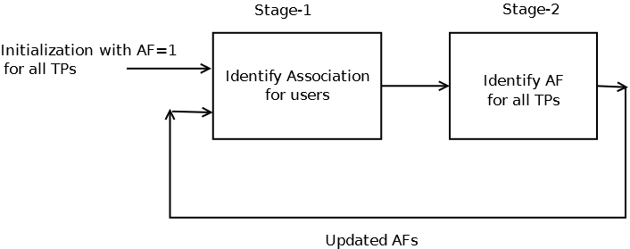
We propose two joint association & AF optimization algorithms for solving the problem in (8). These algorithms follow an alternating optimization approach where user association (stage-1) and AF (stage-2) are optimized in an alternating fashion. Fig. 1 shows a block-level decomposition. The first algorithm is the Joint GLS-AF algorithm, in which we first run the GLS algorithm (Algorithm in Table I) and use the obtained association in our AF optimization algorithm in Section IV . We repeat the following two steps until the benefit in terms of the alpha-fairness system utility falls below a threshold.

  1. 1.

    Stage1–Fix $\bm{\rho}$ and use GLS algorithm to calculate the user association.

  2. 2.

    Stage2–Fix the association and optimize over $\bm{\rho}$ using the auxiliary function method given in Section IV .

It is evident that both stages in the above alternating approach can be performed using the respective distributed versions that we derived before. However, one issue with the proposed joint GLS-AF algorithm, is that the TPs that do not serve any user in any one iteration will be discarded in all subsequent iterations. To overcome this potential limitation, we consider the joint relaxed association and AF (Joint RA-AF) algorithm. To obtain the association, this latter algorithm in stage-1 solves the convex optimization problem obtained by relaxing variables $x_{k,b},\;\forall\;k,b$ in (12) or (13) to be continuous variables in $[0,1]$. In this solution, a user $k$ can have $x_{k,b}$ non-zero for more than one TP $b$. In stage-2, the algorithm fixes $x_{k,b}$ for all $k,b$ and optimizes the AF. To do so, it uses the auxiliary function method of Section IV on the objective in the problem (12) rather than (25) as $x_{k,b}$ can now have fractional values. This two stage procedure is repeated until the benefit in system utility falls below a threshold. Finally, the Joint RA-AF algorithm rounds $x_{k,b}$ to obtain a feasible association.

VI Evaluation

We present a detailed evaluation of our proposed: Greedy Local Search (GLS) algorithm, the distributed Greedy (DG) algorithm and the joint association & AF optimization algorithms over an LTE HetNet deployment. In our evaluation topology an enhanced NodeB (eNB) covers the coordination area. The eNB site comprises of three cells (sectors), where each sector contains a set of eleven TPs formed by one macro and ten lower power (pico) nodes. We drop ninety nine users on the eNB site so there are a total of $B=33$ TPs and $K=99$ users. All TPs and users have a single antenna each. We employ the conservative rates and ignore fast fading in the results presented in Section VI-A & Section VI-B. The results incorporating actual rates, fast fading and efficient per-slot user scheduling are presented later in Section VI-C.

VI-A Association

We compare the GLS & DG algorithms proposed in Section III-A and Section III-B, respectively, to the following:

  • Relaxed Upperbound (RU)–Solves the convex optimization problem obtained by relaxing $x_{k,b}$ in (12) or (13). Though the obtained solution need not be feasible for (LABEL:eq:Bigoriginal), the scheme provides us with an upperbound on the optimal of (LABEL:eq:Bigoriginal).

  • Relaxed Rounded Association (RRA)–Solves the convex optimization problem obtained by relaxing $x_{k,b}$ in (12) or (13). Each user $k$ connects to the TP $b$ corresponding to highest $x_{k,b}$ in the obtained convex optimization solution. This scheme is widely used to represent the performance that can be achieved by a feasible and near-optimal user association scheme. However, it requires solving a convex problem that can be computationally quite complex compared to GLS in a dense deployment.

  • Max SNR Association (MSA)– Each user independently connects to the TP from which it sees the highest average channel gain. This scheme is the most common baseline.

We evaluate the association algorithms by examining their returned utility function values for varying $\alpha$. We also evaluate the additional gain yielded by the local search (LS) stage over the greedy one in the GLS algorithm.

VI-A1 $\alpha\leq 1$

We begin with an evaluation of GLS and the distributed greedy (DG) algorithm in the regime $\alpha\leq 1$, where we consider the maximization of the objective in (13). We set $\rho=1$ for each of the 33 TPs and list the utility values of different association algorithms in Table IV. As suggested by the guarantee in Proposition 2, we observe that greedy stage of GLS itself performs very close to the upper bound RU, and hence close to the optimal and provides good gains over the MSA scheme. Notice that GLS outperforms the RRA despite having a much lower computational complexity. Moreover, the DG algorithm performs close to the former two ones, while simultaneously offering the benefits of a distributed implementation. We also observe that the local search iterations (LSIs) of GLS are at-most 1 and that there is a slight utility gain obtained by the LS stage. Interestingly, upon employing the association algorithm from [12] we observed that the GLS indeed yields the optimal association for this example when $\alpha=1$.

$\alpha$ Greedy GLS RU RRA MSA DG LSI
0.25 67.75 67.82 67.82 67.82 65.08 67.48 1
0.5 112.67 112.67 112.71 112.52 107.03 110.39 0
0.75 288.57 288.57 288.82 288.46 277.65 283.98 0
1.0 -133.93 -133.87 -133.3 1 -133.93 -154.67 -139.76 1
TABLE IV: Utility versus $\alpha$

VI-A2 $\alpha>1$

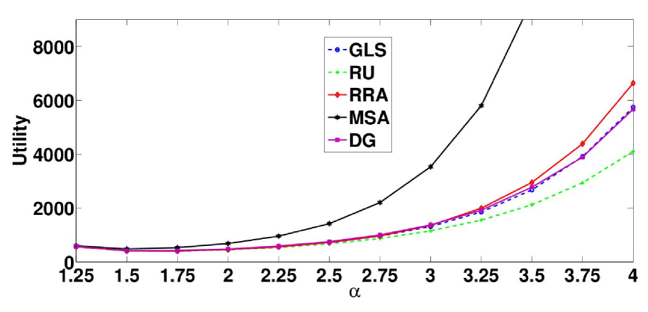
Next we study the performance of GLS & DG algorithms in $\alpha>1$ region, where we consider the minimization of the objective in (12). As seen in Fig. 2(a) the proposed GLS & DG perform very similarly and they noticeably outperform RRA in $\alpha>3$ regime while beating MSA over the entire range of $\alpha>1$. For example, GLS performs 13.5 % better than RRA and 80% better than MSA at $\alpha=4$. MSA performs poorly throughout the $\alpha>1$ regime since it has a naive user specific view rather than an optimized system specific view. The superiority of GLS & DG over RRA & MSA increases with increase in $\alpha$. For example, at a high $\alpha=10$, which approaches max-min fairness, the GLS outperforms RRA & MSA by 93.2% and 100% respectively.
In Table V we study the advantage of doing local search in the $\alpha>1$ region. It is known that the greedy algorithm does not yield a constant factor approximation for the constrained minimization of a non-negative non-decreasing supermodular set function. 111This problem is equivalent to the constrained maximization of a submodular set function albeit where that set function is not non-negative and non-decreasing, so that the classical result [30] is inapplicable. Therefore, the greedy stage need not be close to the optimal and there is room for improvement by the LS stage. As seen in Table V, though the number of LS iterations are at-most 2, the order of gain over the greedy is upto 3.6%. At a higher $\alpha=10$ the gain of GLS over greedy shoots up to 43%, with the number of LS iterations equal to 5. Therefore, as $\alpha$ is progressively increased, the local search stage of the GLS algorithm becomes increasingly important.

$\alpha$ Greedy GLS LSI
1.25 563.9 563.9 0
1.5 411.4 411.3 1
1.75 408.7 406.8 2
2.0 462.6 458.9 2
2.25 565.6 559.0 2
2.5 728.5 717.2 2
$\alpha$ Greedy GLS LSI
2.75 975.2 956.1 2
3.0 1345.8 1314.2 2
3.25 1904.6 1853.0 2
3.5 2754.6 2671.2 2
3.75 4045.1 3911.4 2
4.0 5953.6 5740.7 2
TABLE V: Local Search Improvement
Refer to caption
2(a) Utility vs $\alpha$
Refer to caption
2(b) Utility vs iterations

VI-B Joint Association & Activation fraction optimization

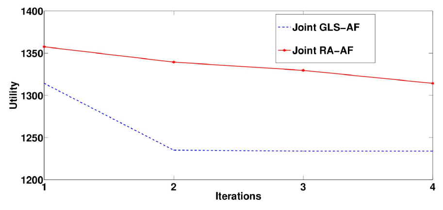
In Fig. 2(b) we study the performance of the two joint algorithms described in Section V for $\alpha=3.0$ for up-to 4 iterations. Each point in the plot corresponds to an iteration, and is the utility value obtained using the updated association, where that association itself is calculated using the updated value of the activation fractions. The value at the first iteration is the utility corresponding to the association done using AF equal to 1 for all TPs. In the Joint RA-AF, at every iteration we calculate the utility by rounding the fractional association as done in the RRA algorithm. However, as mentioned in Section V, fractional values of the association variables $\{x_{k,b}\}$ are passed on to its second stage of AF identification. MSA with $\rho=1$ for each TP with a utility value of 3531.8, performs much worse than the Joint GLS-AF & Joint RA-AF schemes. We obtain a gain of 6.1% for Joint GLS-AF over the case when we do only association via GLS with a fixed $\bm{\rho=1}$, which demonstrates the benefit of doing the joint association and AF optimization. The Joint RA-AF scheme performs worse (upto 8.45%) than the Joint GLS-AF algorithm at every iteration, illustrating that the benefits of GLS over RRA observed before at $\bm{\rho=1}$ are preserved even in the joint optimization problem.
For $\alpha=0.5$, Joint GLS-AF performs 23.36% better than MSA with $\bm{\rho=1}$, as compared to the gain of 4.6% obtained by GLS over MSA observed in Table IV, again demonstrating the gain of optimizing AF and the association jointly. We observe that Joint GLS-AF & Joint RRA-AF algorithms perform very close to each other in $\alpha<1$ regime. This is because of the similar performance of GLS and RRA schemes in this $\alpha$ regime.

VI-C Result Verification with Fast Fading

Finally, in this section we incorporate fast fading and efficient per-slot user scheduling to asses the benefits of the association and activation fractions calculated using proposed Joint GLS-AF algorithm. In particular, we assume that each frame comprises of $5000$ slots and model all fast fading coefficients seen by each user on each slot as i.i.d. complex normal ${\mathcal{C}}{\mathcal{N}}(0,1)$ variables. We randomly generate an ON-OFF pattern (for slots across each frame) for each TP that is compliant with its assigned activation fraction. Further, each TP employs the per-slot gradient based scheduling policy [29] over the set of users associated to it in order to maximize the utility. Then, using the actual per-user average rates so obtained, we compute the system utility values for different schemes. For $\alpha=0.5$ we observed that the Joint GLS-AF scheme yields a $15.35\%$ gain over the baseline scheme (MSA with ${\bm{\rho}}={{\mathbf{1}}}$), while the gain of the GLS with ${\bm{\rho}}={{\mathbf{1}}}$ over the baseline is $5.32\%$. For $\alpha=3$ the gains of these two schemes over the baseline are $47.8\%$ and $39.4\%$, respectively. This validates that our approach to obtain the association and AF does indeed result in significant gains in the presence of fast fading and efficient fine time-scale (per-slot) scheduling.

VII Conclusion

We analyzed and evaluated novel association and activation fraction optimization algorithms for maximizing the alpha-fairness utility in HetNets. We derived useful performance guarantees and demonstrated the significant benefits of our proposed algorithms over a practical HetNet topology.

Appendix A Appendix: Definitions

We capture some basic definitions that are used in this paper.

Definition 1.

Given a ground set $\Omega$, we define its power set (i.e., the set containing all the subsets of $\Omega$) as $2^{\Omega}$. Then, a real-valued function defined on the subsets of $\Omega$, $h:2^{\Omega}\to{{\mathrm{I}\!R}}$ is normalized if $h(\phi)=0$, where $\phi$ denotes the empty set. It is called a submodular set function if and only if

$\displaystyle h({\mathcal{B}}\cup a)-h({\mathcal{B}})\leq h({\mathcal{A}}\cup a)-h({\mathcal{A}}),$
$\displaystyle\;\forall\;{\mathcal{A}}\subseteq{\mathcal{B}}\subseteq\Omega\;\&\;a\in\Omega\setminus{\mathcal{B}}$

and a supermodular set function if and only if

$\displaystyle h({\mathcal{B}}\cup a)-h({\mathcal{B}})\geq h({\mathcal{A}}\cup a)-h({\mathcal{A}}),$
$\displaystyle\;\forall\;{\mathcal{A}}\subseteq{\mathcal{B}}\subseteq\Omega\;\&\;a\in\Omega\setminus{\mathcal{B}}.$

A non-negative valued set function $h:2^{\Omega}\to{{\mathrm{I}\!R}}_{+}$ is a non-decreasing set function if and only if it satisfies, $0\leq h({\mathcal{A}})\leq h({\mathcal{B}}),\;\forall\;{\mathcal{A}}\subseteq{\mathcal{B}}\subseteq\Omega$.

Definition 2.

$(\Omega,{\underline{I}})$ is said to be a partition matroid when there exists a partition $\Omega=\cup_{i=1}^{J}\Omega_{i}$, where $\Omega_{i}\cap\Omega_{j}=\phi,\;\forall\;i\neq j$, along with integers $n_{i}\geq 1\;\forall\;i$ such that

$\displaystyle{\mathcal{B}}\subseteq\Omega:|{\mathcal{B}}\cap\Omega_{i}|\leq n_{i}\;\forall\;i\Leftrightarrow{\mathcal{B}}\in{\underline{I}}.$ (31)

Proof of (8)

We will show in brief that for each TP $b\in{\mathcal{B}}$

$\displaystyle\begin{split}&\mbox{max}_{\gamma_{k,b}\in[0,1]\;\forall\;k\atop\sum_{k\in{\mathcal{U}}}\gamma_{k,b}=1}\left\{\sum_{k\in{\mathcal{U}}}x_{k,b}\left(w_{k}u(\gamma_{k,b}R_{k,b}({\bm{\rho}}))\right)\right\}=\\ &-\left(\sum_{k\in{\mathcal{U}}}x_{k,b}\left(w_{k}\frac{(R_{k,b}({\bm{\rho}}))^{1-\alpha}}{\alpha-1}\right)^{1/\alpha}\right)^{\alpha}\end{split}$ (32)

The lagrangian for the convex optimization problem stated above is given by

$\displaystyle\begin{split}&\sum_{k\in{\mathcal{U}}}\frac{-x_{k,b}w_{k}{(\gamma_{k,b}R_{k,b}({\bm{\rho}}))}^{1-\alpha}}{\alpha-1}+\sum_{k\in{\mathcal{U}}}{\lambda_{k}(\gamma_{k,b})}\\ &+\mu(1-\sum_{k\in{\mathcal{U}}}{\gamma_{k,b}})\end{split}$ (33)

Using the first order derivative conditions and complementary slackness conditions, it is seen that the objective attains maximum value when for each user $k:x_{k,b}=1$, $\lambda_{k}=0$ so that $\gamma_{k,b}>0$, and the following conditions are satisfied.

$\displaystyle\begin{split}&w_{k}{(\gamma_{k,b})}^{-\alpha}{R_{k,b}({\bm{\rho}})}^{1-\alpha}=\mu,\;\forall\;k:x_{k,b}=1;\\ &\sum_{k\in{\mathcal{U}}:x_{k,b}=1}\gamma_{k,b}=1\end{split}$ (34)

Solving for optimal $\gamma_{k,b}$ from (34) and putting its value back in the objective, we obtain the RHS of (11).

Proposition 1:
Hardness of User Association: The hardness of the user association sub-problem for a fixed ${\bm{\rho}}$ can be shown via a reduction from the partition problem. To show this, we consider the case $\alpha>1$ and suppose that there is an optimal polynomial time user association algorithm. Further, we restrict ourselves to input instances in which the rates that all users can obtain from two distinct TPs $b1,b2\in{\mathcal{B}}$ are identical to one, whereas the rate that each user can obtain from any other TP is zero. Thus, we assume that $R_{k,b}({\bm{\rho}})=1,\;\forall\;k\in{\mathcal{U}}\;\&\;b\in\{b1,b2\}$ while $R_{k,b}({\bm{\rho}})=0,\;\forall\;k\in{\mathcal{U}}\;\&\;b\in{\mathcal{B}}\setminus\{b1,b2\}$. We allow the user weights to be any input set of positive scalars that sum to 1. Then, the problem in (12) simplifies to

$\displaystyle\begin{split}&\mbox{min}_{x_{k,b}\in\{0,1\}\;\forall\;k\in{\mathcal{U}},b\in\{b1,b2\}\atop\sum_{b\in\{b1,b2\}}x_{k,b}=1\;\forall\;k}\left\{\sum_{b\in\{b1,b2\}}\left(\sum_{k\in{\mathcal{U}}}x_{k,b}w_{k}^{1/\alpha}\right)^{\alpha}\right\}.\end{split}$ (35)

Then, defining $\hat{z}=\arg\min_{z\in[0,1]}\{z^{\alpha}+(1-z)^{\alpha}\}$, it is readily verified that $\hat{z}$ is unique and equal to $1/2$, with $\hat{z}^{\alpha}+(1-\hat{z})^{\alpha}=2^{1-\alpha}$. Letting $W=\sum_{k\in{\mathcal{U}}}w_{k}^{1/\alpha}$, this implies that the objective value in (35) returned by the optimal polynomial time user association algorithm will be equal to $W^{\alpha}2^{1-\alpha}$ if and only if there exists a partition of the set of user weights (each raised to power $1/\alpha$) into two parts that have an identical sum. This in turn implies that the algorithm at hand is an optimal polynomial time algorithm for the NP-complete partition problem. Indeed, suppose $\{y_{1},\cdots,y_{K}\}:\;y_{k}>0,\;\forall k$ is any input set to the latter problem where we need to determine if there exists a partition of that set into two parts of identical sum. Setting $w_{k}=\frac{y_{k}^{\alpha}}{\sum_{i=1}^{K}y_{i}^{\alpha}},\;\forall\;k=1,\cdots,K$, we obtain a valid input set of weights for (35). Then, from the output of the supposed optimal algorithm at hand, we can immediately determine if there is such a partition for the set $\{\frac{y_{k}}{(\sum_{i=1}^{K}y_{i}^{\alpha})^{1/\alpha}}\}_{k=1}^{K}$ and thus the set $\{y_{k}\}_{k=1}^{K}$, which yields the desired contradiction. The same reduction can be established for $\alpha=1$ as well as $\alpha\in(0,1)$.

To prove the remaining parts of this proposition, we note that $x^{\alpha}$ for all non-negative $x$ is concave in $x$ when $\alpha\in(0,1)$ and convex in $x$ when $\alpha>1$. Then, we note the fact that composition of a non-negative modular set function with a concave (convex) function yields a submodular (supermodular) set function. Further, submodularity as well as supermodularity is preserved under set restriction and the sum of submodular (supermodular) functions is submodular (supermodular). Using these facts, we obtain the desired results. Similarly, for $\alpha=1$ we note that $-x\ln(x)$ is concave in $x$ for all non-negative $x$. This fact along with the aforementioned arguments and the fact that the sum of a submodular set function and a modular set function is submodular, establishes the proof in this case. Finally, since we allow for arbitrarily small (albeit positive) $R_{k,b}({\bm{\rho}})$ for any tuple $(k,b)$ the set function $g(.,1)$ need not be non-decreasing nor non-negative.

Before we consider Proposition 2, we state and prove a lemma that will invoked later. The bounds given in this lemma are applicable to arbitrary submodular or supermodular set functions.

Lemma 1:
For any given $\alpha$, the greedy stage yields an output $\hat{{\underline{\mathcal{G}}}}$ such that

$\displaystyle\begin{split}&g(\hat{{\underline{\mathcal{G}}}},\alpha)\geq g({\underline{\mathcal{G}}}^{\rm opt}\cup\hat{{\underline{\mathcal{G}}}},\alpha)-g(\hat{{\underline{\mathcal{G}}}}\setminus{\underline{\mathcal{G}}}^{\rm opt},\alpha),\;\;\forall\;\alpha\in(0,1]\\ &g(\hat{{\underline{\mathcal{G}}}},\alpha)\leq g({\underline{\mathcal{G}}}^{\rm opt}\cup\hat{{\underline{\mathcal{G}}}},\alpha)-g(\hat{{\underline{\mathcal{G}}}}\setminus{\underline{\mathcal{G}}}^{\rm opt},\alpha),\;\;\forall\;\alpha>1.\end{split}$ (36)
Proof.

We prove the first relation in (36). For notational convenience let us denote a tuple as ${\underline{e}}=(k,b)$. We expand $\hat{{\underline{\mathcal{G}}}}$ as $\hat{{\underline{\mathcal{G}}}}=\{\hat{{\underline{e}}}_{1},\hat{{\underline{e}}}_{2},\cdots,\hat{{\underline{e}}}_{K}\}$ where $\hat{{\underline{e}}}_{i}$ denotes the tuple added at the $i^{th}$ greedy step and let $\delta_{i},\;i=1,\cdots,K$ denote the associated change in system utility. Further, we define the sets $\hat{{\underline{\mathcal{G}}}}_{i}=\{\hat{{\underline{e}}}_{1},\hat{{\underline{e}}}_{2},\cdots,\hat{{\underline{e}}}_{i}\},\;\forall\;\;i=1,\cdots,K$ with $\hat{{\underline{\mathcal{G}}}}_{0}=\phi$. Then, note that both ${\underline{\mathcal{G}}}^{\rm opt},\hat{{\underline{\mathcal{G}}}}\in{\underline{{\bm{\mathcal{I}}}}}$ and are maximal members in ${\underline{{\bm{\mathcal{I}}}}}$, i.e., $|{\underline{\mathcal{G}}}^{\rm opt}|=|{\underline{\mathcal{G}}}|=K$. Further, using the definitions given above, we see that ${\underline{{\bm{\mathcal{I}}}}}$ is a partition matroid. Invoking a result on maximal members in a matroid (cf. [31]), we can deduce that without loss of generality, we can expand ${\underline{\mathcal{G}}}^{\rm opt}=\{{\underline{e}}^{\rm opt}_{1},{\underline{e}}^{\rm opt}_{2},\cdots,{\underline{e}}^{\rm opt}_{K}\}$ such that for each $i\in\{1,\cdots,K\}$,

$\displaystyle{\rm Either}\;{\underline{e}}^{\rm opt}_{i}=\hat{{\underline{e}}}_{i},\;\;{\rm or}\;\;$
$\displaystyle{\underline{e}}^{\rm opt}_{i}\notin\hat{{\underline{\mathcal{G}}}}\;\&\;(\hat{{\underline{\mathcal{G}}}}\setminus\hat{{\underline{e}}}_{i})\cup{\underline{e}}^{\rm opt}_{i}\in{\underline{{\bm{\mathcal{I}}}}}.$ (37)

Then, letting $\tilde{{\underline{\mathcal{G}}}}\stackrel{{\scriptstyle\scriptscriptstyle\triangle}}{{=}}\hat{{\underline{\mathcal{G}}}}\setminus{\underline{\mathcal{G}}}^{\rm opt}$ we have the chain of inequalities (38) given on the top of the next page which yields the desired result.

$\displaystyle\begin{split}g(\hat{{\underline{\mathcal{G}}}},\alpha)=\sum_{i=1}^{K}\delta_{i}=\sum_{i:\hat{{\underline{e}}}_{i}\in\hat{{\underline{\mathcal{G}}}}\cap{\underline{\mathcal{G}}}^{\rm opt}}(g(\hat{{\underline{\mathcal{G}}}}_{i-1}\cup\hat{{\underline{e}}}_{i},\alpha)-g(\hat{{\underline{\mathcal{G}}}}_{i-1},\alpha))+\sum_{i:\hat{{\underline{e}}}_{i}\in\tilde{{\underline{\mathcal{G}}}}}(g(\hat{{\underline{\mathcal{G}}}}_{i-1}\cup\hat{{\underline{e}}}_{i},\alpha)-g(\hat{{\underline{\mathcal{G}}}}_{i-1},\alpha))\\ \geq\sum_{i:\hat{{\underline{e}}}_{i}\in\hat{{\underline{\mathcal{G}}}}\cap{\underline{\mathcal{G}}}^{\rm opt}}(g(\hat{{\underline{\mathcal{G}}}}_{i-1}\cup\tilde{{\underline{\mathcal{G}}}}\cup\hat{{\underline{e}}}_{i},\alpha)-g(\hat{{\underline{\mathcal{G}}}}_{i-1}\cup\tilde{{\underline{\mathcal{G}}}},\alpha))+\sum_{i:\hat{{\underline{e}}}_{i}\in\tilde{{\underline{\mathcal{G}}}}}(g(\hat{{\underline{\mathcal{G}}}}_{i-1}\cup\hat{{\underline{e}}}_{i},\alpha)-g(\hat{{\underline{\mathcal{G}}}}_{i-1},\alpha))\\ =g(\hat{{\underline{\mathcal{G}}}},\alpha)-g(\tilde{{\underline{\mathcal{G}}}},\alpha)+\sum_{i:\hat{{\underline{e}}}_{i}\in\tilde{{\underline{\mathcal{G}}}}}(g(\hat{{\underline{\mathcal{G}}}}_{i-1}\cup\hat{{\underline{e}}}_{i},\alpha)-g(\hat{{\underline{\mathcal{G}}}}_{i-1},\alpha))\\ \geq g(\hat{{\underline{\mathcal{G}}}},\alpha)-g(\tilde{{\underline{\mathcal{G}}}},\alpha)+\sum_{i:{\underline{e}}^{\rm opt}_{i}\notin\hat{{\underline{\mathcal{G}}}}}(g(\hat{{\underline{\mathcal{G}}}}_{i-1}\cup{\underline{e}}^{\rm opt}_{i},\alpha)-g(\hat{{\underline{\mathcal{G}}}}_{i-1},\alpha))\\ \geq g(\hat{{\underline{\mathcal{G}}}},\alpha)-g(\tilde{{\underline{\mathcal{G}}}},\alpha)+\sum_{i:{\underline{e}}^{\rm opt}_{i}\notin\hat{{\underline{\mathcal{G}}}}}(g(\hat{{\underline{\mathcal{G}}}}\cup{\underline{e}}^{\rm opt}_{i},\alpha)-g(\hat{{\underline{\mathcal{G}}}},\alpha))\\ \geq g(\hat{{\underline{\mathcal{G}}}},\alpha)-g(\tilde{{\underline{\mathcal{G}}}},\alpha)+g({\underline{\mathcal{G}}}^{\rm opt}\cup\hat{{\underline{\mathcal{G}}}},\alpha)-g(\hat{{\underline{\mathcal{G}}}},\alpha),\end{split}$ (38)

In (38) the first inequality follows from submodularity of $g(.,\alpha)$ and the fact that for each $i:\hat{{\underline{e}}}_{i}\in\hat{{\underline{\mathcal{G}}}}\cap{\underline{\mathcal{G}}}^{\rm opt}$, $\hat{{\underline{\mathcal{G}}}}_{i-1}\subseteq\hat{{\underline{\mathcal{G}}}}_{i-1}\cup\tilde{{\underline{\mathcal{G}}}}$ and $\hat{{\underline{e}}}_{i}\notin\hat{{\underline{\mathcal{G}}}}_{i-1}\cup\tilde{{\underline{\mathcal{G}}}}$. The second inequality follows from (A) along with the fact that for each $i:{\underline{e}}^{\rm opt}_{i}\notin\hat{{\underline{\mathcal{G}}}}$, the greedy algorithm would have considered ${\underline{e}}^{\rm opt}_{i}$ but choose $\hat{{\underline{e}}}_{i}$ instead since the latter offered a better (greater) change in system utility. The third inequality also follows from submodularity of $g(.,\alpha)$ and the fact that each $i:{\underline{e}}^{\rm opt}_{i}\notin\hat{{\underline{\mathcal{G}}}}$ we have $\hat{{\underline{\mathcal{G}}}}_{i-1}\subseteq\hat{{\underline{\mathcal{G}}}}$, and the final inequality also follows from submodularity of $g(.,\alpha)$. Note that none of the steps require $g(.,\alpha)$ to be a non-negative set function or that the changes in system utility should be non-negative. The second relation in (36) can be proved in an analogous fashion.∎

Proposition 2:
For any given $\alpha$, the greedy stage yields an output $\hat{{\underline{\mathcal{G}}}}$ such that

$\displaystyle\begin{split}&g(\hat{{\underline{\mathcal{G}}}},\alpha)\geq g({\underline{\mathcal{G}}}^{\rm opt},\alpha)/2\;\;\forall\;\alpha\in(0,1),\\ &g(\hat{{\underline{\mathcal{G}}}},\alpha)\geq g({\underline{\mathcal{G}}}^{\rm opt},\alpha)-2\ln(2)\;\;\forall\;\alpha=1,\\ &(3-2^{\alpha})g(\hat{{\underline{\mathcal{G}}}},\alpha)\leq g({\underline{\mathcal{G}}}^{\rm opt},\alpha)\;\;\forall\;\alpha>1.\end{split}$ (39)
Proof.

For $\alpha\in(0,1)$, since $g(.,\alpha)$ is submodular and non-decreasing, we can readily obtain (39) from (36) by observing that $g({\underline{\mathcal{G}}}^{\rm opt}\cup\hat{{\underline{\mathcal{G}}}},\alpha)\geq g({\underline{\mathcal{G}}}^{\rm opt},\alpha)$ and $g(\hat{{\underline{\mathcal{G}}}},\alpha)\geq g(\hat{{\underline{\mathcal{G}}}}\setminus{\underline{\mathcal{G}}}^{\rm opt},\alpha)$. Note that (39) is the classical result derived earlier [30]. For $\alpha=1$, the result in (39) is novel and thus more interesting. To prove (39), we first re-write the bound in (36) as

$\displaystyle\begin{split}g(\hat{{\underline{\mathcal{G}}}},1)\geq g({\underline{\mathcal{G}}}^{\rm opt},1)+g({\underline{\mathcal{G}}}^{\rm opt}\cup\hat{{\underline{\mathcal{G}}}},1)-g({\underline{\mathcal{G}}}^{\rm opt},1)\\ -g(\hat{{\underline{\mathcal{G}}}}\setminus{\underline{\mathcal{G}}}^{\rm opt},1).\end{split}$ (40)

Then, recall from (17) that $g(.,1)$ is the sum of a modular function and a submodular function where the latter depends only on the user weights, and the sum of these weights across all users is unity. Consequently, we can infer that

$\displaystyle\begin{split}&g({\underline{\mathcal{G}}}^{\rm opt}\cup\hat{{\underline{\mathcal{G}}}},1)-g({\underline{\mathcal{G}}}^{\rm opt},1)-g(\hat{{\underline{\mathcal{G}}}}\setminus{\underline{\mathcal{G}}}^{\rm opt},1)\\ =&-\sum_{b}(x_{b}+y_{b})\ln(x_{b}+y_{b})+\sum_{b}(z_{b}+y_{b})\ln(z_{b}+y_{b})\\ &+\sum_{b}(x_{b}-z_{b})\ln(x_{b}-z_{b})\end{split}$ (41)

where $x_{b}$ is the sum of weights of users associated to TP $b$ by the greedy solution (and hence is known), $y_{b}+z_{b}$ is the sum of weights of users associated to TP $b$ by the optimal solution and $z_{b}$ is the sum of weights of users associated to TP $b$ by both the greedy and the optimal solutions. Note further that $\sum_{b}x_{b}=\sum_{b}(y_{b}+z_{b})=1$. Combining (41) with (40) we can obtain the following specialized bound,

$\displaystyle\begin{split}g(\hat{{\underline{\mathcal{G}}}},1)\geq&g({\underline{\mathcal{G}}}^{\rm opt},1)\\ &+\min_{y_{b},z_{b}\geq 0;z_{b}\leq x_{b}\;\forall b\atop\sum_{b}(y_{b}+z_{b})=1}\{-\sum_{b}(x_{b}+y_{b})\ln(x_{b}+y_{b})\\ &+\sum_{b}(z_{b}+y_{b})\ln(z_{b}+y_{b})\\ &+\sum_{b}(x_{b}-z_{b})\ln(x_{b}-z_{b})\}.\end{split}$ (42)

Then, by using the K.K.T. conditions for the optimization problem in the RHS of (42), it can be shown that the minima is attained at $y_{b}=x_{b}\;\&\;z_{b}=0\;\forall\;b$ so that

$\displaystyle\begin{split}&\min_{y_{b},z_{b}\geq 0;z_{b}\leq x_{b}\;\forall b\atop\sum_{b}(y_{b}+z_{b})=1}\{-\sum_{b}(x_{b}+y_{b})\ln(x_{b}+y_{b})\\ &+\sum_{b}(z_{b}+y_{b})\ln(z_{b}+y_{b})+\sum_{b}(x_{b}-z_{b})\ln(x_{b}-z_{b})\}=-2\ln(2).\end{split}$

This proves the result in (39). Next, we consider $\alpha>1$ and specialize the bound in (36) as

$$g(\hat{{\underline{\mathcal{G}}}},\alpha)\leq g({\underline{\mathcal{G}}}^{\rm opt},\alpha)+g({\underline{\mathcal{G}}}^{\rm opt}\cup\hat{{\underline{\mathcal{G}}}},\alpha)-g({\underline{\mathcal{G}}}^{\rm opt},\alpha)-g(\hat{{\underline{\mathcal{G}}}}\setminus{\underline{\mathcal{G}}}^{\rm opt},\alpha)\\ =g({\underline{\mathcal{G}}}^{\rm opt},\alpha)+\sum_{b}((v_{b}+t_{b})^{\alpha}-(v_{b}+u_{b})^{\alpha}\\ -(t_{b}-u_{b})^{\alpha}),$$ (43)

where now $t_{b}$ is the sum of gains of all users associated to TP $b$ by the greedy solution (i.e., sum of $\Theta_{k}^{(b)}(\alpha)$ in (III) for all tuples in $\hat{{\underline{\mathcal{G}}}}\cap\Omega^{(b)}$ and hence is known) so that $g(\hat{{\underline{\mathcal{G}}}},\alpha)=\sum_{b}t_{b}^{\alpha}$. $v_{b}+u_{b}$ is the sum of gains of all users associated to TP $b$ by the optimal solution and $u_{b}$ is the sum of gains of all users associated to TP $b$ by both the greedy and the optimal solutions. Clearly, then we can further bound

$\displaystyle\begin{split}g(\hat{{\underline{\mathcal{G}}}},\alpha)\leq g({\underline{\mathcal{G}}}^{\rm opt},\alpha)+&\max_{v_{b},u_{b}\geq 0;u_{b}\leq t_{b}\;\forall b\atop\sum_{b}(v_{b}+u_{b})^{\alpha}\leq g(\hat{{\underline{\mathcal{G}}}},\alpha)}\{\sum_{b}((v_{b}+t_{b})^{\alpha}\\ &-(v_{b}+u_{b})^{\alpha}-(t_{b}-u_{b})^{\alpha})\}\end{split}$ (44)

Again invoking the K.K.T. conditions for the optimization problem in the RHS of (44), it can be shown that the maxima is attained at $v_{b}=t_{b}\;\&\;u_{b}=0\;\forall\;b$ so that

$\displaystyle\begin{split}&\max_{v_{b},u_{b}\geq 0;u_{b}\leq t_{b}\;\forall b\atop\sum_{b}(v_{b}+u_{b})^{\alpha}\leq g(\hat{{\underline{\mathcal{G}}}},\alpha)}\{\sum_{b}\left((v_{b}+t_{b})^{\alpha}-(v_{b}+u_{b})^{\alpha}-(t_{b}-u_{b})^{\alpha}\right)\}\\ &=(2^{\alpha}-2)g(\hat{{\underline{\mathcal{G}}}},\alpha)\end{split}$ (45)

This then proves the result in (39).∎

Proposition 3:
The GLS algorithm for any given $\Delta\geq 0$ yields an output $\breve{{\underline{\mathcal{G}}}}$ such that for any given $\alpha>1$

$\displaystyle\begin{split}&g({\underline{\mathcal{G}}}^{\rm opt},\alpha)\geq g(\breve{{\underline{\mathcal{G}}}},\alpha)+K{(1-\Delta)g(\breve{{\underline{\mathcal{G}}}},\alpha)}-h(\breve{{\underline{\mathcal{G}}}},\alpha)\\ \end{split}$

and for any given $\alpha\in(0,1)$

$\displaystyle\begin{split}&g({\underline{\mathcal{G}}}^{\rm opt},\alpha)\leq g(\breve{{\underline{\mathcal{G}}}},\alpha)+K{(1+\Delta)g(\breve{{\underline{\mathcal{G}}}},\alpha)}-h(\breve{{\underline{\mathcal{G}}}},\alpha).\\ \end{split}$

Further, for $\alpha=1$

$\displaystyle g({\underline{\mathcal{G}}}^{\rm opt},1)\leq\;\;\;\;\;\;\;\;\;\;\;\;\;\;\;\;$
$\displaystyle g(\breve{{\underline{\mathcal{G}}}},1)+K{(1+\Delta{\mathrm{sgn}}(g(\breve{{\underline{\mathcal{G}}}},1)))g(\breve{{\underline{\mathcal{G}}}},1)}-h(\breve{{\underline{\mathcal{G}}}},1),$ (46)

where, $h(\breve{{\underline{\mathcal{G}}}},\alpha)=\sum_{n=1}^{K}g(\breve{{\underline{\mathcal{G}}}}\setminus\breve{{\underline{e}}}_{n},\alpha)+\sum_{n=1}^{K}(g(\tilde{{\underline{\Omega}}},\alpha)-g(\tilde{{\underline{\Omega}}}\setminus\breve{{\underline{e}}}_{n},\alpha))$, for any subset $\tilde{{\underline{\Omega}}}\subseteq{\underline{\Omega}}:{\underline{\mathcal{G}}}^{\rm opt}\cup\breve{{\underline{\mathcal{G}}}}\subseteq\tilde{{\underline{\Omega}}}$.

Proof.

We prove the result for $\alpha>1$ and the result for $\alpha$ in other regimes can be derived similarly. We again invoke a result on maximal members in a matroid [31], to deduce that without loss of generality, we can expand $\breve{{\underline{\mathcal{G}}}}=\{\breve{{\underline{e}}}_{1},\breve{{\underline{e}}}_{2},\cdots,\breve{{\underline{e}}}_{K}\}$ and expand ${\underline{\mathcal{G}}}^{\rm opt}=\{{\underline{e}}^{\rm opt}_{1},{\underline{e}}^{\rm opt}_{2},\cdots,{\underline{e}}^{\rm opt}_{K}\}$ such that for some $m\in\{0,1,\cdots,K\}$,

$\displaystyle{\underline{e}}^{\rm opt}_{n}=\breve{{\underline{e}}}_{n},\;\;\forall\;n\leq m\;\;\&\;\;{\underline{e}}^{\rm opt}_{n}\neq\breve{{\underline{e}}}_{n},\;\;\forall\;n>m$
$\displaystyle(\breve{{\underline{\mathcal{G}}}}\setminus\breve{{\underline{e}}}_{n})\cup{\underline{e}}^{\rm opt}_{n}\in{\underline{{\bm{\mathcal{I}}}}},\;\forall\;n:m+1\leq n\leq K.$ (47)

Then, we have the following inequalities for each $n=m+1,\cdots,K$.

$\displaystyle\begin{split}g(\breve{{\underline{\mathcal{G}}}}\cup{\underline{e}}^{\rm opt}_{n},\alpha)-g(\breve{{\underline{\mathcal{G}}}},\alpha)&\geq g((\breve{{\underline{\mathcal{G}}}}\setminus\breve{{\underline{e}}}_{n})\cup{\underline{e}}^{\rm opt}_{n},\alpha)-g(\breve{{\underline{\mathcal{G}}}}\setminus\breve{{\underline{e}}}_{n},\alpha)\\ &\geq(1-\Delta)g(\breve{{\underline{\mathcal{G}}}},\alpha)-g(\breve{{\underline{\mathcal{G}}}}\setminus\breve{{\underline{e}}}_{n},\alpha)\end{split}$ (48)

where the first inequality follows from the supermodularity of $g(.,\alpha)$ and the second one follows from the local swap optimality of $\breve{{\underline{\mathcal{G}}}}$, i.e.,

$\displaystyle g((\breve{{\underline{\mathcal{G}}}}\setminus\breve{{\underline{e}}}_{n})\cup{\underline{e}}^{\rm opt}_{n},\alpha)-g(\breve{{\underline{\mathcal{G}}}},\alpha)\geq-\Delta g(\breve{{\underline{\mathcal{G}}}},\alpha).$ (49)

Thus, we have that

$\displaystyle\begin{split}&\sum_{n=m+1}^{K}(g(\breve{{\underline{\mathcal{G}}}}\cup{\underline{e}}^{\rm opt}_{n},\alpha)-g(\breve{{\underline{\mathcal{G}}}},\alpha))\\ &\geq\sum_{n=m+1}^{K}((1-\Delta)g(\breve{{\underline{\mathcal{G}}}},\alpha)-g(\breve{{\underline{\mathcal{G}}}}\setminus\breve{{\underline{e}}}_{n},\alpha))\end{split}$ (50)

and due to the supermodularity of $g(.,\alpha)$,

$\displaystyle\begin{split}&\sum_{n=m+1}^{K}g(\breve{{\underline{\mathcal{G}}}}\cup{\underline{e}}^{\rm opt}_{n},\alpha)-g(\breve{{\underline{\mathcal{G}}}},\alpha)\\ &\leq\sum_{n=m+1}^{K}(g(\breve{{\underline{\mathcal{G}}}}\cup\{{\underline{e}}^{\rm opt}_{m+1},\cdots,{\underline{e}}^{\rm opt}_{n}\},\alpha)\\ &-g(\breve{{\underline{\mathcal{G}}}}\cup\{{\underline{e}}^{\rm opt}_{m+1},\cdots,{\underline{e}}^{\rm opt}_{n-1}\},\alpha)\\ &=g(\breve{{\underline{\mathcal{G}}}}\cup{\underline{\mathcal{G}}}^{\rm opt},\alpha)-g(\breve{{\underline{\mathcal{G}}}},\alpha).\end{split}$ (51)

Next, we have the bound

$\displaystyle\begin{split}&g(\breve{{\underline{\mathcal{G}}}}\cup{\underline{\mathcal{G}}}^{\rm opt},\alpha)\\ &=g({\underline{\mathcal{G}}}^{\rm opt},\alpha)+\sum_{n=m+1}^{K}(g({\underline{\mathcal{G}}}^{\rm opt}\cup\{\breve{{\underline{e}}}_{m+1},\cdots,\breve{{\underline{e}}}_{n}\},\alpha)\\ &-g({\underline{\mathcal{G}}}^{\rm opt}\cup\{\breve{{\underline{e}}}_{m+1},\cdots,\breve{{\underline{e}}}_{n-1}\},\alpha)\\ &\leq g({\underline{\mathcal{G}}}^{\rm opt},\alpha)+\sum_{n=m+1}^{K}(g(\tilde{{\underline{\Omega}}},\alpha)-g(\tilde{{\underline{\Omega}}}\setminus\breve{{\underline{e}}}_{n},\alpha)),\end{split}$ (52)

for any subset $\tilde{{\underline{\Omega}}}\subseteq{\underline{\Omega}}:{\underline{\mathcal{G}}}^{\rm opt}\cup\breve{{\underline{\mathcal{G}}}}\subseteq\tilde{{\underline{\Omega}}}$. Combining the bounds in (48), (51) and (52) we get

$$g({\underline{\mathcal{G}}}^{\rm opt},\alpha)\geq g(\breve{{\underline{\mathcal{G}}}},\alpha)+\sum_{n=m+1}^{K}((1-\Delta)g(\breve{{\underline{\mathcal{G}}}},\alpha)-g(\breve{{\underline{\mathcal{G}}}}\setminus\breve{{\underline{e}}}_{n},\alpha))\\ -\sum_{n=m+1}^{K}(g(\tilde{{\underline{\Omega}}},\alpha)-g(\tilde{{\underline{\Omega}}}\setminus\breve{{\underline{e}}}_{n},\alpha)).$$ (53)

The RHS of (53) is further lower bounded to obtain the desired result in (A), by extending the summation from $1$ to $K$, where we note that each term $((1-\Delta)g(\breve{{\underline{\mathcal{G}}}},\alpha)-g(\breve{{\underline{\mathcal{G}}}}\setminus\breve{{\underline{e}}}_{n},\alpha))-(g(\tilde{{\underline{\Omega}}},\alpha)-g(\tilde{{\underline{\Omega}}}\setminus\breve{{\underline{e}}}_{n},\alpha))\leq 0$ since $\Delta\geq 0$ and $g(.,\alpha)$ is supermodular and non-negative. ∎

Proposition 4:

For non-negative non-decreasing submodular set functions, which we recall does not hold for our set functions when $\alpha\geq 1$, a somewhat lesser known result is that a restricted version of the greedy algorithm can also yield identical constant factor approximation [32]. We next establish a similar result with respect to the bounds in Lemma 1 and Proposition 2. In particular, we first detail the restricted greedy algorithm in Table VI.

TABLE VI: Restricted Greedy Algorithm
1:  Initialize with any ordering $\pi(.)$ defined on ${\mathcal{U}}$ and $\hat{{\underline{\mathcal{G}}}}^{\rm rg}=\phi$.
2:  For $k=1\;{\rm to}\;K$,
3:  Determine $(\pi(k),b^{\prime})$ as the tuple in ${\underline{\Omega}}$ which offers the best change among all tuples $(\pi(k),b)\in{\underline{\Omega}}$.
4:  Update $\hat{{\underline{\mathcal{G}}}}^{\rm rg}=\hat{{\underline{\mathcal{G}}}}^{\rm rg}\cup(\pi(k),b^{\prime})$.
5:  End For.
6:  Output $\hat{{\underline{\mathcal{G}}}}^{\rm rg}$.

Next, we show that for any given ordering $\pi(.)$, the restricted greedy algorithm yields a solution that also satisfies the bounds in Lemma 1 for all $\alpha$. Thus, the solution of the restricted greedy algorithm also satisfies the bounds in Proposition 2 for all $\alpha$ and hence yields the same firm guarantees for all $\alpha\in\left(0,\frac{\ln(3)}{\ln(2)}\right)$. Towards this end, we expand the solution yielded by the restricted greedy algorithm as $\hat{{\underline{\mathcal{G}}}}^{\rm rg}=\{\hat{{\underline{e}}}^{{\rm rg},\pi}_{1},\hat{{\underline{e}}}^{{\rm rg},\pi}_{2},\cdots,\hat{{\underline{e}}}^{{\rm rg},\pi}_{K}\}$ where $\hat{{\underline{e}}}^{{\rm rg},\pi}_{i}$ denotes the tuple added at the $i^{th}$ step as per the ordering $\pi(.)$. Then, notice that all the arguments in the proof of Lemma 1 go through even upon replacing $\hat{{\underline{\mathcal{G}}}}$ with $\hat{{\underline{\mathcal{G}}}}^{\rm rg}$ and $\hat{{\underline{e}}}_{i}$ with $\hat{{\underline{e}}}^{{\rm rg},\pi}_{i},\;\forall\;i$. The key point to note here is that we do not require the changes in system utility obtained across the steps to be ordered. In other words, we do not use the fact that these changes obtained during the greedy stage of the GLS algorithm are ordered as $\delta_{1}\geq\delta_{2}\geq\cdots\geq\delta_{K}$ when $\alpha\leq 1$ or as $\delta_{1}\geq\delta_{2}\geq\cdots\geq\delta_{K}$ when $\alpha>1$, whereas no such ordering is ensured for those obtained during the restricted greedy algorithm.

Notice that the the aforementioned result applies to any ordering $\pi(.)$. We will exploit this fact along with a result that the solution yielded by the distributed greedy algorithm maps exactly to that yielded by the restricted greedy algorithm for a particular ordering. We will suppose that $\alpha\leq 1$ since the arguments we make directly extend to the case where $\alpha>1$. Let $\hat{{\underline{e}}}^{\rm dg}_{1},\cdots,\hat{{\underline{e}}}^{\rm dg}_{K}$ be the tuples selected by the distributed greedy algorithm, where we assume that tuples $\hat{{\underline{e}}}^{\rm dg}_{1},\cdots,\hat{{\underline{e}}}^{\rm dg}_{m1}$ are selected in the first window, tuples $\hat{{\underline{e}}}^{\rm dg}_{m1+1},\cdots,\hat{{\underline{e}}}^{\rm dg}_{m2}$ are selected in the second window and so on. Moreover, let $u_{1},u_{2},\cdots,u_{m1}$ denote the corresponding users in the tuples selected in the first window, let $u_{m1+1},u_{m1+2},\cdots,u_{m2}$ denote the corresponding users in the tuples selected in the second window and so on. We define an ordering $\pi(.)$ such that $\pi(k)=u_{k},\;k=1,\cdots,K$. Note here that we can pick any arbitrary order to list the users (tuples) selected by the distributed greedy algorithm within each window. We will show that

$\displaystyle\hat{{\underline{e}}}^{{\rm rg},\pi}_{k}=\hat{{\underline{e}}}^{\rm dg}_{k},\;\forall\;k=1,\cdots,K$ (54)

which proves the desired result. Consider the tuples selected in the first window. Each user $u_{i}\;i=1,\cdots,m1$ chooses the TP yielding the best change in system utility assuming zero current load on all TPs. Thus, it is readily seen that $\hat{{\underline{e}}}^{{\rm rg},\pi}_{1}=\hat{{\underline{e}}}^{\rm dg}_{1}$. Consider the TP choice of user $u_{i},\;i=2,\cdots,m1$ made as $\hat{{\underline{e}}}^{\rm dg}_{i}=\arg\max_{(u_{i},b),b\in{\mathcal{B}}}\{g((u_{i},b),\alpha)\}$. By sub-modularity of $g(.,\alpha)$ for $\alpha\leq 1$ and the fact that the TPs chosen by the admitted users in each window are all distinct, we have that

$\displaystyle\hat{{\underline{e}}}^{\rm dg}_{i}=\arg\max_{(u_{i},b),b\in{\mathcal{B}}}\left\{g(\{\hat{{\underline{e}}}^{\rm dg}_{1}\cup\cdots\cup\hat{{\underline{e}}}^{\rm dg}_{i-1}\}\cup(u_{i},b),\alpha)-\right.$
$\displaystyle\left.g(\{\hat{{\underline{e}}}^{\rm dg}_{1}\cup\cdots\cup\hat{{\underline{e}}}^{\rm dg}_{i-1}\},\alpha)\right\}.\;$ (55)

Put differently, given that tuples $\{\hat{{\underline{e}}}^{\rm dg}_{1}\cup\cdots\cup\hat{{\underline{e}}}^{\rm dg}_{i-1}\}$ have been already chosen, the best TP for user $u_{i}$ will still be the one in $\hat{{\underline{e}}}^{\rm dg}_{i}$. This is because upon selecting the tuples $\{\hat{{\underline{e}}}^{\rm dg}_{1}\cup\cdots\cup\hat{{\underline{e}}}^{\rm dg}_{i-1}\}$ the loads of the TPs in these tuples will increase, whereas that of the one in $\hat{{\underline{e}}}^{\rm dg}_{i}$ will remain unchanged. Thus, the system utility change obtained if user $u_{i}$ joined each one of those TPs (given these selections) will be inferior, respectively, to what that user assumed when making its decision (since it used a lower value of the load). On the other hand, the system utility change obtained if user $u_{i}$ joined the TP in $\hat{{\underline{e}}}^{\rm dg}_{i}$ (given that tuples $\{\hat{{\underline{e}}}^{\rm dg}_{1}\cup\cdots\cup\hat{{\underline{e}}}^{\rm dg}_{i-1}\}$ have been already selected) will be identical to what it assumed. Then, from (A) we have that $\hat{{\underline{e}}}^{{\rm rg},\pi}_{i}=\hat{{\underline{e}}}^{\rm dg}_{i},\;\forall\;i=1,\cdots,m1$. The same argument applies to each subsequent window upon observing that all users that are selected in that window use load values that account for all associations made in all prior windows. Thus, we can conclude that (54) is true which proves our claim for the distributed greedy algorithm.

In this context, we note that another distributed greedy algorithm can be obtained by altering the TP-side procedure to one where in each window each TP admits only the user offering the best change among all users that have requested it in that window. From the proof detailed above, it can be verified that this variant also yields identical performance guarantees.

Distributed LS Stage:

We will show that this distributed LS stage provably converges and the solution it yields upon convergence yields the same guarantees in Proposition 3.

To prove this claim, we define a system state to be a feasible user association, i.e., an association where each user is associated to one TP. Thus, the set of all possible system states is finite and comprises of all feasible user associations. Let us define a system state to be an absorbing state if at that state, for each user the switch yielding the best change in system utility (21) does not yield a relative improvement better than $\Delta$ (cf. (22) and (23)). Clearly, the optimal system state (which yields the globally optimal system utility) is an absorbing state so that the set of absorbing states is finite and non-empty. Further, given any non-absorbing state it can be verified that we can construct a finite sequence of states that begins at the given state and ends at an absorbing one, such that each transition from any state to the next one in that sequence involves a migration of exactly one user and yields a relative improvement (in the system utility) better than $\Delta$.

Next, considering the distributed LS algorithm, it is readily seen that the broadcast of the current load information at the start of each window corresponds to a system state. Moreover, without loss of generality, we can assume that each user which sends a request in any window is accepted with a strictly positive probability that depends only on the system state at the begining of that window and the user index. Consequently, the sequence of states seen across the broadcast slots forms an absorbing, time homogeneous Markov Chain. Hence, convergence to an absorbing state is guaranteed. Indeed, the expected number of steps for convergence can be obtained from the analysis in [33]. Finally, since the bound in Proposition 3 is satisfied by any absorbing state, we can assert the claimed guarantee for the distributed LS algorithm is true.

AF Optimization

We first discuss a distributed implementation that ensures no loss in performance. Towards this end, it is readily seen that for any fixed activation vector ${\bm{\rho}}$ the optimization over $\bf{s,g}$ decouples into smaller problems which can be separately solved at each TP. We notice, however, that the AF variables in the GP formulation in (30) induce coupling constraints. Nevertheless, this issue can be addressed by exploiting a useful decomposition technique from [34] and introducing local copies for the AF variables. In particular, for each AF variable $\rho_{b}$, we introduce $B-1$ local copies $\rho_{b^{\prime},b},\;\forall\;b^{\prime}\in{\mathcal{B}}:b^{\prime}\neq b$ ($\rho_{b^{\prime},b}$ is the copy of $\rho_{b}$ maintained at TP $b^{\prime}$) and re-write the GP in (30) including these local copies along with equality constraints $\rho_{b}=\rho_{b^{\prime},b},\;\forall\;b^{\prime}\in{\mathcal{B}}:b^{\prime}\neq b,\forall\;b\in{\mathcal{B}}$, as the following.

$$\begin{split}&\mbox{min}_{\{\rho_{b},\{\rho_{b,b^{\prime}}\}\},{\bf z},{\bf t}}\{\sum_{b\in{B}}{z_{b}^{\alpha}}\}\\ &\mbox{subject to}\\ &\sum_{k\in{\mathcal{U}}^{(b)}}{z_{b}^{-1}\tilde{w}_{k}t_{k,b}^{1/\alpha-1}}\leq{1}\ \ \forall\;b\in{\mathcal{B}}\\ &\frac{t_{k,b}\rho_{b}^{-1}+\mathbb{E}[s_{k,b}({\bm{\beta}}_{k})e_{k,b}({\bm{\beta}}_{k},\rho_{b},\{\rho_{b,b^{\prime}}\})]}{1+\mathbb{E}[\log(s_{k,b}({\bm{\beta}}_{k}))]}\leq 1,\forall\;k\in{\mathcal{U}}^{(b)},b\in{\mathcal{B}}\\ &\rho_{b^{\prime}}=\rho_{b,b^{\prime}},\;\forall\;b^{\prime}\neq b\;\&\;b\in{\mathcal{B}}.\end{split}$$ (56)

The problem in (57) can be decomposed into smaller sub-problems by using a Lagrange multiplier for each equality constraint (a.k.a. consistency price variable). However, to ensure that the sub-problems are also convex, we first adopt the (usual) change of variables $\tilde{z}_{b}=\ln(z_{b})$, $\tilde{t}_{k,b}=\ln(t_{k,b}),\;\forall\;k\in{\mathcal{U}}^{(b)}$, $\tilde{\rho}_{b}=\ln(\rho_{b})$ and $\tilde{\rho}_{b,b^{\prime}}=\ln(\rho_{b,b^{\prime}}),\;\forall\;b^{\prime}\neq b$, for all $b\in{\mathcal{B}}$. Then, we note that the equality constraints can be written as $\tilde{\rho}_{b^{\prime}}=\tilde{\rho}_{b,b^{\prime}}$ forall $b^{\prime}\neq b\;\&\;b\in{\mathcal{B}}$. This transformed problem is presented below

$$\begin{split}&\mbox{min}_{\{\tilde{\rho}_{b},\{\tilde{\rho}_{b,b^{\prime}}\}\},{\bf\tilde{z}},{\bf\tilde{t}}}\sum_{b\in{B}}{\exp(\alpha\tilde{z}_{b})}\\ &\mbox{subject to}\\ &\ln(\sum_{k\in{\mathcal{U}}^{(b)}}{\tilde{w}_{k}\exp(-\tilde{z}_{b}+(1/\alpha-1)\tilde{t}_{k,b})})\leq{0}\ \ \forall\;b\in{\mathcal{B}}\\ &\ln\left(\frac{\exp(\tilde{t}_{k,b}-\tilde{\rho}_{b})+\mathbb{E}[s_{k,b}({\bm{\beta}}_{k})\tilde{e}_{k,b}({\bm{\beta}}_{k},\tilde{\rho}_{b},\{\tilde{\rho}_{b,b^{\prime}}\})]}{1+\mathbb{E}[\log(s_{k,b}({\bm{\beta}}_{k}))]}\right)\leq 0,\forall\;k,b\\ &\tilde{\rho}_{b^{\prime}}=\tilde{\rho}_{b,b^{\prime}},\;\forall\;b^{\prime}\neq b\;\&\;b\in{\mathcal{B}}.\end{split}$$ (57)

where we use $\tilde{e}_{k,b}(.,.)$ to denote the MSE as function of the transformed variables. Note that (57) a convex optimization problem with its utility function (decoupled across TPs) and where the constraints are either also decoupled or are coupled linear equality ones. Thus, a decomposition technique introduced in [34] is now directly applicable and accordingly we introduce a Lagrange multiplier for each equality constraint constraint. Each TP $b$ can then separately solve a convex sub-problem and the multipliers can be updated using the sub-gradient method in a distributed manner [34].

A-A $\alpha=1$

AF optimization problem over the set of variables $\bm{\rho}=\{\rho_{b}\}\;\forall b\in{B}$ in $\alpha=1$ regime is given by

$\displaystyle\mbox{maximize}_{{\bm{\rho}}\in{\bf{[0,1]}}}$ $\displaystyle\left\{\sum_{b\in{B}}{\sum_{k\in{{\mathcal{U}}^{(b)}}}{w_{k}\ln(R_{k,b}({\bm{\rho}}))}}\right\}$ (58)

The problem of interest is equivalent to

$\displaystyle\mbox{minimize}_{{\bm{\rho}}\in{\bf{[0,1]}}}$ $\displaystyle\left\{\sum_{b\in{B}}{\sum_{k\in{{\mathcal{U}}^{(b)}}}{w_{k}\ln(\frac{1}{R_{k,b}({\bm{\rho}})})}}\right\}$ (59)

As done in case of $\alpha>1$, we reduce (59) and fix $\bf{s,g}$ to obtain

$$\begin{split}&\mbox{min}_{\bm{\rho}\in{\bf{[0,1]}},{\bf t}\geq{\bf 0}}\left\{\sum_{b\in{B}}\sum_{k\in{{\mathcal{U}}^{(b)}}}{w_{k}\ln(t_{k,b})^{-1}}\right\}\\ &\mbox{subject to}\\ &\frac{t_{k,b}\rho_{b}^{-1}+\mathbb{E}(s_{k,b}({\bm{\beta}}_{k})e_{k,b}({\bm{\beta}}_{k},{\bm{\rho}}))}{1+\mathbb{E}(\log(s_{k,b}({\bm{\beta}}_{k})))}\leq 1\ \ \forall{b,k}\end{split}$$ (60)

We consider change of variables $t_{k,b}=\exp({\tilde{t}_{k,b}})\;\forall{b}\in{B},k\in{{\mathcal{U}}^{(b)}}$ and $\rho_{b}=\exp({\tilde{\rho}_{b}})\ \forall b\in{B}$. Let $a_{k,b}=\frac{1}{1+\mathbb{E}(\log{s_{k,b}({\bm{\beta}}_{k}))}}$. Now (60) can be further reduced to

$$\begin{split}&\mbox{min}_{\tilde{\bm{\rho}}\leq{\bf{0}},\tilde{\bm{t}}}\left\{\sum_{b\in{B}}{\sum_{k\in{{\mathcal{U}}^{(b)}}}{-w_{k}\tilde{t}_{k,b}}}\right\}\\ &\mbox{subject to}\\ &\log(a_{k,b}\exp{(-\tilde{\rho}_{b}+\tilde{t}_{k,b})}\\ &+a_{k,b}\mathbb{E}(s_{k,b}({\bm{\beta}}_{k})(\left|g_{k,b}({\bm{\beta}}_{k})\sqrt{\beta_{k,b}}-1\right|^{2}+\left|g_{k,b}({\bm{\beta}}_{k})\right|^{2}))\\ &+\sum_{b^{\prime}\neq b}\exp(\tilde{\rho}_{b^{\prime}})a_{k,b}\mathbb{E}(s_{k,b}({\bm{\beta}}_{k})\left|g_{k,b}({\bm{\beta}}_{k})\right|^{2}{\beta_{k,b^{\prime}}}))\leq{0}\end{split}$$ (61)

Note that (61) is a convex optimization problem. Again, we use alternating optimization approach to obtain the solution of (58). We use solution of (27) to minimize over $\bm{s,g}$ when $\bm{\rho}$ is fixed and further use (61) to minimize over $\bm{\rho}$ when $\bm{s,g}$ are fixed.

A-B $\alpha<1$

AF optimization problem over the set of variables $\bm{\rho}=\{\rho_{b}\}\;\forall b\in{B}$ in $\alpha\in{(0,1)}$ regime is given by

$\displaystyle\mbox{max}_{{\bm{\rho}}\in{\bf{[0,1]}}}$ $\displaystyle\left\{\sum_{b\in{B}}{(\sum_{k\in{{\mathcal{U}}^{(b)}}}{\tilde{w}_{k}(R_{k,b}({\bm{\rho}}))^{1/\alpha-1}})^{\alpha}}\right\}$ (62)

Where $\tilde{w}_{k}=(\frac{w_{k}}{1-\alpha})^{1/\alpha}$. We choose $C=\sum_{b\in{B}}{(\sum_{k\in{{\mathcal{U}}^{(b)}}}{\tilde{w}_{k}(\mathbb{E}(\log(1+\beta_{k,b})))^{1/\alpha-1}})^{\alpha}}$. Now we use the reduction for (62) as done in (27)-(29) and further fix $\bf{s}$ and $\bf{g}$. We obtain the following optimization problem in variables $\bm{\rho},{\bf z},{\bf t}$

$$\begin{split}&\mbox{min}_{{\bm{\rho}}\in{\bf{[0,1]}},{\bf z}\geq{\bf 0},{\bf t}\geq{\bf 0}}\ \ C-\sum_{b\in{B}}{z_{b}^{\alpha}}\\ &\mbox{subject to}\\ &z_{b}\leq{\sum_{k\in{{\mathcal{U}}^{(b)}}}{\tilde{w}_{k}t_{k,b}^{1/\alpha-1}}}\ \ \forall{b}\\ &\frac{t_{k,b}\rho_{b}^{-1}+\mathbb{E}(s_{k,b}({\bm{\beta}}_{k})e_{k,b}({\bm{\beta}}_{k},{\bm{\rho}}))}{1+\mathbb{E}(\log(s_{k,b}({\bm{\beta}}_{k})))}\leq 1\ \ \forall{b,k}\end{split}$$ (63)

Adding an extra variable $y$, the above problem (63) is equivalent to

$$\begin{split}&\mbox{minimize}_{{y}{\geq 0},{\bm{\rho}}\in{\bf{[0,1]}},{\bf z}\geq{\bf 0},{\bf t}\geq{\bf 0}}\ \ \left\{y\right\}\\ &\mbox{subject to}\\ &{\frac{C}{y+\sum_{b\in{B}}{z_{b}^{\alpha}}}\leq 1}\\ &\frac{z_{b}}{{\sum_{k\in{{\mathcal{U}}^{(b)}}}{\tilde{w}_{k}t_{k,b}^{1/\alpha-1}}}}\leq 1\forall{b}\\ &\frac{t_{k,b}\rho_{b}^{-1}+\mathbb{E}(s_{k,b}({\bm{\beta}}_{k})e_{k,b}({\bm{\beta}}_{k},{\bm{\rho}}))}{1+\mathbb{E}(\log(s_{k,b}({\bm{\beta}}_{k})))}\leq 1\ \ \forall{b,k}\end{split}$$ (64)

To transform this optimization problem (64) into a GP, we need to apply the single condensation method [35] on the first two constraints of (64), which are of the form of ratio of a monomial and a posynomial. Let $\bm{X}=(y,\bm{z})$ and $\bm{t}=\{t_{k,b}\}\ \ \forall b\in{B},\forall{k}\in{{\mathcal{U}}^{(b)}}$. For any current $\tilde{\bf{X}},\tilde{\bf{t}}$ we define

$\displaystyle\tilde{f}(\bm{X})=(\frac{yf(\tilde{\bm{X}})}{\tilde{y}})^{\frac{\tilde{y}}{f(\tilde{\bm{X}})}}\prod_{b}{(\frac{z_{b}^{\alpha}f(\tilde{\bm{X}})}{\tilde{z}_{b}^{\alpha}})^{\frac{\tilde{z}_{b}^{\alpha}}{f(\tilde{\bm{X}})}}}$ (65)

Where $f(\tilde{\bm{X}})=\tilde{y}+\sum_{b\in{B}}{\tilde{z}_{b}^{\alpha}}$. We also define

$\displaystyle\tilde{h}_{b}(\bm{t})=\prod_{{k}\in{{\mathcal{U}}^{(b)}}}{(\frac{t_{k,b}^{1/\alpha-1}h_{b}(\tilde{\bm{t}})}{\tilde{t}_{k,b}^{1/\alpha-1}})^{\frac{\tilde{t}_{k,b}^{1/\alpha-1}\tilde{w}_{k}}{h_{b}(\tilde{\bm{t}})}}}$ (66)

Where $h_{b}(\tilde{\bm{t}})=\sum_{{k}\in{{\mathcal{U}}^{(b)}}}{\tilde{w}_{k}\tilde{t}_{k,b}^{1/\alpha-1}}$. Then the following approximate problem is a GP

$$\begin{split}&\mbox{minimize}_{{\bm{X}}{\geq 0},{\bm{\rho}}\in{\bm{[0,1]}},{\bm{t}}\geq{\bm{0}}}\left\{y\right\}\\ &\mbox{subject to}\\ &{\frac{C}{\tilde{f}(\bm{X})}\leq 1}\\ &\frac{z_{b}}{\tilde{h}_{b}(\bm{t})}\leq 1\ \ \forall{b}\\ &\frac{t_{k,b}\rho_{b}^{-1}+\mathbb{E}(s_{k,b}({\bm{\beta}}_{k})e_{k,b}({\bm{\beta}}_{k},{\bm{\rho}}))}{1+\mathbb{E}(\log(s_{k,b}({\bm{\beta}}_{k})))}\leq 1\ \ \forall{b,k}\end{split}$$ (67)

References

  • [1] 3GPP, “Study on small cell enhancements for E-UTRA and E-UTRAN – physical-layer aspects,” TR36.872 V12.0.0, Sept. 2013.
  • [2] A. Gjendemsjoe, D. Gesbert, G. Oien, and S. Kiani, “Binary power control for sum rate maximization over multiple interfering links,” IEEE Trans. Wireless. Comm., Aug. 2008.
  • [3] W. Yu, T. Kwon, and C. Shin, “Multicell coordination via joint scheduling, beamforming and power spectrum adaptation,” in Proc. IEEE INFOCOM, pp. 2570–2578, Apr. 2011.
  • [4] O. Ayach El, A. Lozano, and R. Heath, “On the overhead of interference alignment: Training, feedback, and cooperation,” IEEE Trans. on Wireless Comm., Nov. 2012.
  • [5] Y. Huang, G. Zheng, M. Bengtsson, K.-K. Wong, L. Yang, and B. Ottersten, “Distributed multicell beamforming with limited intercell coordination,” IEEE Trans. on Sig. Proc., Jan. 2011.
  • [6] M. Sanjabi, M. Razaviyayn, and Z. Q. Luo, “Optimal joint base station assignment and beamforming for heterogeneous networks,” IEEE Trans. on Sig. Proc., Apr. 2014.
  • [7] A. Tajer, N. Prasad, and X. Wang, “Robust linear precoder design for multi-cell downlink transmission,” IEEE Trans. on Signal Processing, jan 2011.
  • [8] N. Vaidhiyan, R. Subramanian, and R. Sundaresan, “Interference planning for multicell OFDM downlink,” in IEEE Comsnets (invited), 2011.
  • [9] H. Kim, G. de Veciana, X. Yang, and M. Venkatachalam, “Distributed $\alpha-$optimal user association and cell load balancing in wireless networks,” IEEE Trans. on Network., Feb. 2012.
  • [10] R. Madan, J. Borran, A. Sampath, N. Bhushan, A. Khandekar, and T. Ji, “Cell association and interference coordination in heterogeneous LTE-A cellular networks,” IEEE J. Sel. Areas Comm., Dec. 2010.
  • [11] K. Shen and W. Yu, “Distributed pricing-based user association for downlink heterogeneous cellular networks,” IEEE Journal Sel. Areas. Commun., Jun. 2014.
  • [12] N. Prasad, M. Arslan, and S. Rangarajan, “Exploiting cell dormancy and load balancing in LTE hetnets: Optimizing the proportional fairness utility,” IEEE Trans. on Commun., Oct. 2014.
  • [13] Q. Ye, B. Rong, Y. Chen, M. Al-Shalash, C. Caramanis, and J. Andrews, “User association for load balancing in heterogeneous cellular networks,” IEEE Trans. on Wireless Comm., June 2013.
  • [14] T. Bu, L. Li, and R. Ramjee, “Generalized proportional fair scheduling in third generation wireless data networks,” IEEE Infocom, 2006.
  • [15] L. Li, M. Pal, and Y. R. Yang, “Proportional fairness in multi-rate wireless LANs,” IEEE Infocom, 2008.
  • [16] K. Son, S. Chong, and G. Veciana, “Dynamic association for load balancing and interference avoidance in multi-cell networks,” IEEE Trans. Wireless Comm., 2009.
  • [17] D. Bethanabhotla, O. Bursalioglu, H. Papadopoulos, and G. Caire, “Optimal user-cell association for massive mimo wireless networks,” v2, arXiv, feb 2015.
  • [18] E. Aryafar, A. Keshavarz-Haddad, M. Wang, and M. Chiang, “RAT selection games in hetnets,” in IEEE Infocom, 2013.
  • [19] N. Prasad, M. Arslan, and S. Rangarajan, “A two time scale approach for coordinated multi-point transmission and reception over practical backhaul,” in IEEE Comsnets (invited), jan 2014.
  • [20] R. Yates, “A framework for uplink power control in cellular radio systems,” IEEE JSAC, Sep. 1995.
  • [21] E. Altman, A. Kumar, C. Singh, and R. Sundaresan, “Spatial sinr games of base station placement and mobile association,” IEEE Infocom., 2009.
  • [22] A. Bedekar and R. Agrawal, “Optimal muting and load balancing for eICIC,” in Proc. IEEE WiOPT, 2013.
  • [23] S. Borst, S. Hanly, and P. Whiting, “Throughput utility optimization in hetnets,” in IEEE VTC, 2013.
  • [24] I. Siomina and D. Yuan, “Analysis of cell load coupling for LTE network planning and optimization,” IEEE Trans. on Wireless Comm., June 2012.
  • [25] A. Fehske and G. Fettweis, “On flow level modeling of multi-cell wireless networks,” in IEEE WiOpt, 2013.
  • [26] X. Lin and N. Shroff, “The impact of imperfect scheduling on cross-layer rate control in wireless networks,” in Proc. IEEE INFOCOM, 2005.
  • [27] S. Deb, A. Keshavarz-Haddad, and V. Srinivasan, “MOTA: engineering an operator agnostic mobile service,” in IEEE Mobicom, 2011.
  • [28] S. Christensen, R. Agarwal, E. Carvalho, and J. Cioffi, “Weighted sum-rate maximization using weighted MMSE for MIMO-BC beamforming design,” IEEE Trans. Wireless Commun., vol. 7, no. 12, pp. 1–8, 2008.
  • [29] A. L. Stolyar, “On the asymptotic optimality of the gradient scheduling algorithm for multi-user throughput allocation,” Operations Res., 2005.
  • [30] G. L. Nemhauser and L. A. Wolsey, “Best algorithms for approximating the maximum of a submodular set function,” Math. Operations Research, 1978.
  • [31] J. Lee, V. Mirrokni, V. Nagarajan, and M. Sviridenko, “Non-monotone submodular maximization under matroid and knapsack constraints,” in STOC, 2009.
  • [32] P. Goundan and A. Schulz, “Revisiting the greedy approach to submodular set function maximization,” manuscript, June 2007.
  • [33] H. Zhang, L. Venturino, N. Prasad, P. Li, S. Rangarajan, and X. Wang, “Weighted sum-rate maximization in multi-cell networks via coordinated scheduling and discrete power control,” IEEE J. Sel. Areas Comm., Dec. 2010.
  • [34] D. P. Palomar and M. Chiang, “A tutorial on decomposition methods for network utility maximization,” IEEE JSAC, Aug. 2006.
  • [35] M. Chiang, Geometric Programming for Communication Systems. Now Publishers, 2005.