From statistics of regular tree-like graphs to distribution function and gyration radius of branched polymers

Abstract

We consider flexible branched polymer, with quenched branch structure, and show that its conformational entropy as a function of its gyration radius $R$, at large $R$, obeys, in the scaling sense, $\Delta S\sim R^{2}/(a^{2}L)$, with $a$ bond length (or Kuhn segment) and $L$ defined as an average spanning distance. We show that this estimate is valid up to at most the logarithmic correction for any tree. We do so by explicitly computing the largest eigenvalues of Kramers matrices for both regular and “sparse” 3-branched trees, uncovering on the way their peculiar mathematical properties.

I Introduction

We are interested in statistical mechanics of long flexible branched objects. The leading example, but certainly not the only one, is large RNA molecule. By means of covalent bonds acting between nucleotides along a chain and non-covalent saturating bonds between complementary bases, RNA molecule folds in a peculiar secondary structure which is effectively a branched polymer. There is an enormous literature on RNA, and on branched polymers in general, however we will be interested in a specific question which has not been sufficiently considered so far: what is the conformational entropy of a branched polymer in a tree-dimensional space, and how does it depend on the overall spatial span (e.g., on the gyration radius), and on the specific arrangement of branches. To make it clear: we imagine a branched polymer, such as a secondary structured RNA, to flex its bonds and junctions without re-arranging secondary structure itself, which we will refer to as quenched branched polymer; we will be interested in entropy associated with spatial conformations of this quenched object.

Conformational entropy of this type was first written down by Daoud et al DaoudPincusStockmayerWitten_1983 , as $\Delta F/T\sim R^{2}/R_{0}^{2}$, where $R$ and $R_{0}$ have been denoted as “actual” and “unperturbed” gyration radii, respectively. In the work DaoudPincusStockmayerWitten_1983 , authors examined the influence of excluded volume interactions on the swelling of branched polymers and on the properties of branched polymers in the solutions, so for them $R$ was the average size of a self-avoiding polymer, while $R_{0}$ was considered as ideal. Actually, $R_{0}$ was taken as $R_{0}\sim aN^{1/4}$, i.e., as a mean size of an ideal tree Zimm_Stockmayer , where averaging was supposed to include both spatial fluctuations of a given tree, and all rearrangements of the tree branches (i.e., it was considered an annealed tree). It is this double average that leads to the well known Zimm-Stockmayer law, $R_{0}\sim aN^{1/4}$, for ideal branched polymers Zimm_Stockmayer .

Later on, a similar looking expression,

$$\Delta F/T\sim R^{2}/(a^{2}L)\ ,$$ (1)

was employed in a more subtle context, emphasizing the difference between quenched and annealed branched polymers Annealed_Branched . In this case, $a^{2}L$ replaces $R_{0}^{2}$. Obviously, in this sense, $L$ can be thought as a length of a Gaussian polymer of a typical mean squared size $\sim R_{0}^{2}$. More meaningfully, $L$ was interpreted as an order parameter, the average spanning distance of a tree. This theory (applied in a variety of contexts Rosa_Everaers_PRL_2014 ; Grosberg_ring_melt_static ; Smrek_Grosberg_annealed_trees_dynamics_2014 ; Bruinsma_virus ) implies the necessity to consider conformational entropy of a branched polymer with fixed (quenched) branches, characterized by $L$. From this point of view, the free energy estimate $\Delta F/T\sim R^{2}/(a^{2}L)$ may seem suspicious. Indeed, if $L$ is the spanning distance of the tree, we can imagine selecting one particular line of exactly $L$ bonds in the tree (call it a tree trunk), and then $R^{2}/(a^{2}L)$ is (or seems to be?) the free energy of this tree trunk viewed as a linear polymer. In fact, to relate this to the free energy of a tree, two aspects have to be taken into account: first, when the tree is stretched (or swollen), then all its branches are stretched, not only the trunk; second, if $R$ is the gyration radius of the tree, then gyration radius of the trunk is somewhat smaller than $R$ (because branches provide a lot of mass close to the center). This leads us to the question: Is the free energy estimate, $\Delta F/T\sim R^{2}/(a^{2}L)$ valid for every tree, with $L$ defined as an average spanning distance, at least in the scaling sense? In this paper, we set out to address this question, and our answer is positive: we will show that this estimate of entropy is valid for any tree, up to at most the logarithmic correction.

We build our arguments based on the so-called Kramers theorem Kramers (see also Rubinstein_book ) and its recent generalization found in Smrek_Grosberg_annealed_trees_dynamics_2014 . These statements can be formulated as follows. Let us label all the bonds of the tree (in arbitrary order) with the index $x$, $1\leq x\leq N-1$, where $N$ is the number of monomers (tree vertices). For a Gaussian system (without excluded volume, and when “bonds” are long enough compared to the persistence length), each bond vector, $\mathbf{a}$, is normally distributed, $\sim e^{-3\mathbf{a}^{2}/2a^{2}}$, with the mean squared bond length $a^{2}=\left<\mathbf{a}^{2}\right>$, where the vectors $\mathbf{a}_{x}$ and $\mathbf{a}_{y}$ are independent for any $x\neq y$. Let us further define the $(N-1)\times(N-1)$ matrix $G$ with the entries $G_{x,y}=M(x)M(y)/N^{2}$, where $M(x)$ and $M(y)$ are the numbers of tree vertices on the one side of bond $x$, while $M(y)$ is the number of vertices on the other side of bond $y$ – see the illustration in the Fig.1 and more detailed discussion in the Section II. In terms of this matrix the Kramers theorem reads:

Kramers theorem.

The averaged gyration radius of the tree is given by the trace ${\rm tr}\,G$:

$$\left<R^{2}/a^{2}\right>=\sum_{x}G_{x,x}=\frac{1}{N^{2}}\sum_{x=1}^{N-1}M(x)(N-M(x))\ .$$ (2)

Here and below, $\left<\ldots\right>$ means quenched average, i.e., average over all spatial conformations with fixed tree structure.

Generalization of Kramers theorem.

For $R\gg\left<R\right>$, the probability $P(R)$ of a given branched polymer (with quenched tree structure) to have a gyration radius $R$, up to power law corrections, goes as

$$\left.P(R)\right|_{R\to\infty}\sim e^{-3R^{2}/(2a^{2}\lambda_{\max})}\ ,$$ (3)

where $\lambda_{\max}$ is the largest eigenvalue of the matrix $G$. In other words, the free energy price for swelling a quenched tree to a large size $R$, up to logarithmic corrections, goes as

$$\Delta F/T\simeq 3R^{2}/(2a^{2}\lambda_{\max})\ .$$ (4)

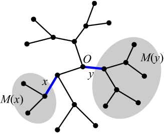
Figure 1: Towards the definition of matrix $G_{x,y}$. On the tree, the bonds $x$ and $y$ naturally divide all nodes of the graph into three categories: on one side of $x$ (shaded), on the other side of $y$ (also shaded), and in between (not shaded). We denote the numbers of monomers in the former two categories as $M(x)$ and $M(y)$. Each matrix element is given by $G_{x,y}=M(x)M(y)/N^{2}$. In this particular example $G_{x,y}=3\times 7/22^{2}$.

The former statement (the Kramers theorem itself) can be also found in the textbook Rubinstein_book , while the latter statement (its generalization) was proven recently in Smrek_Grosberg_annealed_trees_dynamics_2014 . To make the present work self-contained, we reproduce the derivation in the Appendix A.

The result (4) of the generalized Kramers theorem does not explain the relation between $\lambda_{\mathrm{max}}$ and the internal geometry/topology of the tree itself. In this paper we will establish the following:

• For a regularly $p=3$-branching tree (a “3-dendrimer”) $\lambda_{\max}=c_{\rm tree}$ with $c_{\rm tree}\approx 0.957$;

• For a regular sparse tree, where each bond is a linear polymer of length $s$, $\lambda_{\max}=sc_{\rm tree}$;

• For a linear polymer (or palm tree, with trunk, but without branches), $\lambda_{\max}=N/\pi^{2}$;

• We provide an interpolation of $\lambda_{\max}$ from “dense” ($s=1$) to “sparse” $N>s\gg 1$ (almost palm) trees in the form $\lambda_{\max}\simeq\overline{c}s$, where $\overline{c}$ is another constant of order of unity.

• Based on the above examples, we conclude that in general, for any tree, $\lambda_{\mathrm{max}}=\tilde{c}L$, where $L$ is the average spanning distance of the tree, and factor $\tilde{c}$ is at most of the order of $\ln N$.

The last statement makes the bridge between equations (1) and (4), thus proving the former.

II Largest eigenvalue of Kramers matrix for regular trees

II.1 Trees with branchings at every node

To get an explicit form provided by the estimate (4), we computed the highest eigenvalue of adjacency matrix $G$ of a regular symmetric tree. For simplicity we consider $3$-branching trees only, however results can be easily generalized for trees with any branching number, $p$. To specify the system, suppose that the tree has $k$ generations, and the total number of vertices is $N_{k}$. It is convenient to represent a tree by descending levels (generations) as shown in the Fig.2. The distance from the root point, $O$, is counted in the number of levels. In order to construct the adjacency matrix $G$ corresponding to a tree, we should enumerate somehow the tree links. Apparently, the most straightforward and naive is the sequential enumeration of links in each level. Namely, we start with a left-most link in the 1st level and enumerate all links in this generation left-to-the-right, then proceed in the same way with the next level, etc. Thus, all links are enumerated sequentially by natural number $x$, where $x=1,2,...,3\times 2^{k-1}$.

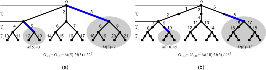
Figure 2: (a) The example of the 3-branching finite tree of $k=3$ levels (generations). Vertices are enumerated by natural numbers sequentially left-to-right in descending order. The shadowed areas mark the subtrees associated with links $x=5$ and $x=3$. The mass of the subtree, $M(x)$, is counted in the number of vertices in this subtree. The matrix element, $G_{x,y}$ of the adjacency matrix $G$ is the product of masses for links $x$ and $y$; (b) An example of “sparse” 3-branching tree of $k=3$ levels. Everything is the same as in (2), however each branching point of the sparse tree is separated by the subchain of $s$ (in the figure (b) $s=2$) links. The tree links are enumerated sequentially first in linear subchains and then – as in (a).

Let us repeat the construction of the adjacency matrix $G=\{G_{x,y}\}$ of the regular tree in the descent diagram representation (Fig.2). Define the “mass,” $M(x)$, associated with the link $x$ as the sum of all vertices in the subtree which begins with the link $x$. The matrix element $G_{x,y}=G_{y,x}$ is the non-normalized product of masses $M(x)$ and $M(y)$ for links $x$ and $y$ correspondingly: $G_{x,y}=M(x)M(y)/N_{3}^{2}$. In the Fig.2 we have demonstrated the construction of the element $G_{3,5}=G_{5,3}$ for the adjacency matrix of size $N_{3}\times N_{3}=22\times 22$. The explicit form of the matrix $G$ for the tree shown in the Fig.2a, is given in the Fig.3a. It is instructive to have a dictionary with necessary definitions:

• The distance from the root point on the tree, counted in the number of levels, is denoted by $j$, the total number of levels in the tree is $k$;

• The total number of vertices, $N_{k}$, of the $k$-level 3-branching tree is $N_{k}=3\times 2^{k}-2$;

• The number of vertices, $N_{j}$, in the subtree starting from some link in the level $j$, is $N_{j,k}=2^{k-j+1}-1$, where $1\geq j\leq k$. (In the Fig.2a the subtrees with $N_{j=2,k=3}=3$ and $N_{j=1,k=3}=7$ are shown). The “mass,” $M$, of the subtree is counted in the number of vertices of this subtree.

The generic structure of the square $N_{k}\times N_{k}$ adjacency matrix $\tilde{G}$ with components $\tilde{G}_{x,y}=N^{2}G_{x,y}\equiv M(x)M(y)$, (where $N_{k}=3\times 2^{k}-2$), is schematically shown in the Fig.3b.

Figure 3: (a) The example of the adjacency matrix $\tilde{G}$ corresponding to the tree in the Fig.2. The matrix $\tilde{G}$ clearly displays a hierarchical structure. By colors we highlight the principal repetitive sequences; (b) The generic structure of the adjacency matrix $\tilde{G}$.

Let us denote by ${\bf U}^{(s)}=\left\{U_{1}^{(s)},...,U_{N_{k}}^{(s)}\right\}$ the eigenvector $s$ of the matrix $G$ corresponding to the eigenvalue $\lambda_{s}$ ($1\leq s\leq N_{k}$), some of eigenvalues and eigenvectors may be degenerated. We noticed that due to the symmetry properties of the adjacency matrix $G$, its leading (maximal) eigenvector $U^{\max}$ has the form

$${\bf U}^{\max}=\Big{\{}\overbrace{U_{1}^{\max},\;U_{1}^{\max},\;U_{1}^{\max}}^{\rm level\;1\;(3\;elements)};\;\overbrace{U_{2}^{\max},\;...,\;U_{2}^{\max}}^{\rm level\;2\;(3\times 2\;elements)};\;...;\;\overbrace{U_{k}^{\max},\;...,\;U_{k}^{\max}}^{{\rm level}\;k\;(3\times 2^{k-1}\;{\rm elements})}\Big{\}}$$ (5)

Plugging this ansatz into the equation $GU^{\max}=\lambda_{\max}U^{\max}$, we find the leading eigenvalue $\lambda_{\max}$ to be also the leading eigenvalue of an exponentially smaller matrix $B$:

$$B\,{\bf V}^{\max}=\lambda_{\max}{\bf V}^{\max}$$ (6)

where ${\bf V}^{\max}=\{U_{1}^{\max},\,U_{2}^{\max},\,...,\,U_{k}^{\max}\}$, and the matrix $B$ reads

$$B=\left(\begin{array}[]{rrrrrr}b_{11}&b_{12}&b_{13}&b_{14}&\ldots&b_{1k}\vskip 6.0pt plus 2.0pt minus 2.0pt\\ \displaystyle\frac{b_{12}}{2}&b_{22}&b_{23}&b_{24}&\ldots&b_{2k}\vskip 6.0pt plus 2.0pt minus 2.0pt\\ \displaystyle\frac{b_{13}}{4}&\displaystyle\frac{b_{23}}{2}&b_{33}&b_{34}&\ldots&b_{3k}\vskip 6.0pt plus 2.0pt minus 2.0pt\\ \displaystyle\frac{b_{14}}{8}&\displaystyle\frac{b_{24}}{4}&\displaystyle\frac{b_{34}}{2}&b_{44}&&b_{4k}\vskip 6.0pt plus 2.0pt minus 2.0pt\\ \vdots&\vdots&\vdots&&\ddots&\vskip 6.0pt plus 2.0pt minus 2.0pt\\ \displaystyle\frac{b_{1k}}{2^{k-1}}&\displaystyle\frac{b_{2k}}{2^{k-2}}&\displaystyle\frac{b_{3k}}{2^{k-3}}&\displaystyle\frac{b_{4k}}{2^{k-4}}&&b_{kk}\end{array}\right);\quad\begin{array}[]{ll}\displaystyle b_{ij}=&2^{-1-2i}(2^{3+k}-3\times 2^{2+i+k}+3\times 2^{2i})\\ &\displaystyle\times\frac{2^{j}-2^{1+k}}{N_{k}^{2}}\qquad(j\geq i)\end{array}$$ (7)

(recall that $N_{k}=3\times 2^{k}-2$). Unlike $G$, which is $N_{k}\times N_{k}$, i.e., exponentially large, the matrix $B$ is only $k\times k$.

In the Fig.4a,b we have plotted the matrix elements of $B$ for $k=5,30$ in form of a 3D relief $B_{i,j}$ over the base plane $(i,j)$, where $(i,j)=1,...,k$. Computing numerically the maximal eigenvalues of the true matrices $B$ defined in (7), for different $k$, we get a plot shown in the Fig.4c.

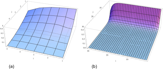
Figure 4: Visualization of the matrix $B$ as a 3D plot of $B_{i,j}$ over the base $(i,j)$ for: (a) $k=5$, (b) $k=30$; (c) Dependence on the maximal eigenvalue of the matrix $B$ (see (7)) of size $k\times k$ on $k$. The limiting value of $\lambda_{\max}$ tends to $\approx 0.957$ as $k\to\infty$.

Extrapolating the data shown in Fig.4 to $k\to\infty$, we obtain

$$\lambda_{\rm max}\approx 0.957$$ (8)

meaning that the largest eigenvalue, $\lambda_{\max}$ of the matrix $B$ and, consequently, of the initial Kramers matrix $G$, is bounded from above by some numeric value independent on the matrix size (and without any logarithmic corrections).

It is noteworthy that a rough estimate of the eigenvalue $\lambda_{\max}$ can be done using the following simple analytical argument. All matrix elements $B_{i,j}$ are positive and

$$B_{i,j}=\left\{\begin{array}[]{ll}b_{i,j}&\quad j\geq i\vskip 6.0pt plus 2.0pt minus 2.0pt\\ b_{j,i}\,2^{i-j}&\quad j<i\end{array}\right.$$

Taking into account the explicit form of matrix elements $b_{i,j}$ for $j\geq i$ (see (7)), we can approximate each element $B_{i,j}$ for any $(i,j)$ by $b_{i,j}$. This approximation gives exact value of $B_{i,j}$ for $j\geq i$, and provides an upper estimate of elements $B_{i,j}$ for $j<i$.

The maximal eigenvalue, $\bar{\lambda}_{\rm max}$, of the $k\times k$ matrix $\bar{B}$ with entries $\{b_{i,j}\}$ can be computed exactly. Eq.(7) means that the element $b_{i,j}$ can be factorized as

$$b_{i,j}=f_{i}\,g_{j};\quad f_{i}=2^{-1-2i}(2^{3+k}-3\times 2^{2+i+k}+3\times 2^{2i});\quad g_{j}=\frac{2^{j}-2^{1+k}}{(3\times 2^{k}-2)^{2}}$$ (9)

Now, the largest eigenvalue, $\bar{\lambda}_{\rm max}$, reads

$$\bar{\lambda}_{\max}=\sum_{m=1}^{k}f_{m}\,g_{m}=\frac{7\times 2^{2+2k}-27k\times 2^{k}-15\times 2^{k}-13}{3(3\times 2^{k}-2)^{2}}$$ (10)

For $k\to\infty$ on gets from (10)

$$\bar{\lambda}_{\max}\Big{|}_{k\to\infty}=\frac{28}{27}\approx 1.037$$ (11)

which is a pretty good approximation for numerically found true limiting value $\lambda_{\max}\approx 0.957$.

II.2 Sparse regular trees

We can generalize our approach to “sparse” regular trees, in which branchings are connected by linear subchains of $s$ links. By definition, for $s=1$ we return to the former case of branching at every node of the tree. Particular example of a dendrimer of $N=19$ nodes with 3-branching vertices separated by 2-link subchains (i.e. $s=2$), is shown in the Fig.2b.

To construct the Kramers adjacency matrix, $G^{(s)}$, for such a tree, one proceeds as above, using the descent diagram representation, where we first enumerate sequentially links in each linear subchain, and then pass to the next subchain in the same level (compare Fig.2a and Fig.2b). The matrix $G^{(s)}$ constructed in such a way, highly resembles the former one, $G$, where each matrix element $G_{x,y}$ is replaced by a $s\times s$–block (a $2\times 2$ block for a particular example of Fig.2b).

The largest eigenvalue, $\lambda_{\max}^{\rm tree}(s)$, of the composite adjacency matrix, $G^{(s)}$, can be estimated as

$$\lambda_{\max}^{\rm tree}(s)\approx\lambda_{\max}^{\rm lin}(s)\;\lambda_{\max}^{\rm tree}$$ (12)

where $\lambda_{\max}^{\rm lin}(s)$ is the maximal eigenvalue of a Kramers matrix for a linear chain of $s$ links and $\lambda_{\max}$ is given by (8). The value of $\lambda_{\max}^{\rm lin}(s)$ reads:

$$\lambda_{\max}^{\rm lin}(s)=\frac{s+1}{4s^{2}}\sin^{-2}\frac{\pi}{2(s+1)};\quad\lambda_{\max}^{\rm lin}(s)=\left\{\begin{array}[]{l}\lambda_{\max}^{\rm lin}(s=1)=1\vskip 6.0pt plus 2.0pt minus 2.0pt\\ \lambda_{\max}^{\rm lin}(s\gg 1)=\frac{s}{\pi^{2}}\end{array}\right.$$ (13)

As it follows from (8), the value $\lambda_{\max}$ can be approximated by some constant, $c$, of order of unity. Thus, we can estimate $\lambda_{\max}^{\rm tree}(s)$ for all regular sparse trees as

$$\lambda_{\max}^{\rm tree}(s)\approx c\lambda_{\max}^{\rm lin}(s)=\bar{c}\,s$$ (14)

where $\bar{c}$ absorbs all numerical constants.

III Discussion

Let us now summarize what we learned about trees. To begin with, recall that for a linear polymer the whole spectrum of the Kramers matrix is known Fixman_1962 (see also small corrections in Fixman_correction_1 and also Fixman_correction_2 ); in particular $\lambda_{\max}=\frac{N}{\pi^{2}}$. Since spanning distance in this case is just $L=N$, we have $\lambda_{\max}=\frac{L}{\pi^{2}}\sim L$.

Next, for the perfect 3-branching dendrimer we have established above that $\lambda_{\max}\approx 1$. This has to be compared with average spanning distance of this tree. For dendrimer with $k$ generations and, accordingly, $3\times 2^{k}$ ends, the sum of distances along a backbone from one end to all other ends is equal to $2+2^{k+1}(3k+1)$. Hence, $L=\frac{1+2^{k}(3k+1)}{3\times 2^{k-1}}$, and at large $k$ this asymptotically tends to $L\simeq 2k$. Since $N=3\times 2^{k+1}-2$, (or, equivalently, $k\simeq\mathrm{log}_{2}\frac{N}{3}-1\simeq\log_{2}N$), we have $L\simeq 2\log_{2}N$. Therefore, we can say that $\lambda_{\max}\approx\frac{L}{2}\log_{2}N$.

Thus, for a regular tree, $\lambda_{\max}$ is related to the average spanning distance $L$ via a factor of order $\ln N$. Let us show now that this is the worst case, and for all other trees the estimate $\lambda_{\max}\sim L$ is even more accurate.

Sparse regular trees provide in this sense a good insight, as they smoothly interpolate between regular tress and linear chains. As we have seen, in this case $\lambda_{\max}\approx s$. On the other hand, in this case $N=3s\left(2^{k+1}-1\right)+1$, or $k=\log_{2}\left[\frac{N+3s-1}{3s}\right]$; at large $N$ this is asymptotic to $k\simeq\log_{2}\left[\frac{N}{s}\right]$. At the same time, $L\simeq 2sk$ or $L\simeq 2s\log_{2}\left[\frac{N}{s}\right]$. Thus,

$$\lambda_{\max}\approx\frac{L}{2}\log_{2}\left[\frac{N}{s}\right]$$

We see that the factor relating $\lambda_{\max}$ to mean spanning distance $L$ smoothly changes between about $\ln N$ and about $1$ as $s$ changes from $1$ to $N$.

In fact, it is clear physically that a regularly branching tree is the most compact and most difficult to swell of all quenched branched polymers, while linear polymer is the least compact and the easiest to swell. Since we have rigorously analyzed both of these extremes, we conclude that the expression (4), which establishes conformational entropy up to logarithmic corrections, implies also the validity of the scaling estimate of entropy (1) in terms of average spanning diameter.

Appendix A Generalized Kramers theorem

Here, we compute the gyration radius probability distribution for a Gaussian tree. The approach follows the works of M. Fixman Fixman_1962 ; Fixman_correction_1 ; Fixman_correction_2 , and Moore_gyration , where it was generalized for Gaussian rings.

Suppose for simplicity that the branching number is $p=3$, and there are only branchings and ends, namely, $n$ three-valent vertices and $n+2$ ends, totally $N=2n+2$ monomers. If ${\bf r}_{i}$ are position vectors of these “monomers,” then the gyration radius reads

$$R^{2}=\frac{1}{2N^{2}}\sum_{i,j}({\bf r}_{i}-{\bf r}_{j})^{2}.$$ (15)

On the tree, every ${\bf r}_{i}-{\bf r}_{j}$ is uniquely represented as the sum of the set of bond vectors ${\bf a}_{i}={\bf r}_{i^{\prime}}-{\bf r}_{i}$, where $i$ and $i^{\prime}$ are monomers connected by bond $k$. Accordingly, gyration radius can be represented as

$$R^{2}=\sum_{x,y}G_{x,y}{\bf a}_{x}{\bf a}_{y},$$ (16)

where the indices $x$ and $y$ label bonds (unlike $i$, $i^{\prime}$ and $j$ above, which label vertices or monomers), and $G_{x,y}$ is an Kramers $(N-1)\times(N-1)$ matrix, illustrated in the Fig.1.

For a Gaussian tree we can do more and find the probability distribution of $R^{2}$, assuming each bond has the probability distribution $\sim e^{-3{\bf a}^{2}/2a^{2}}$. The characteristic function of $R^{2}$ reads

$$\Phi(s)=\left<e^{isR^{2}}\right>=A\int d^{3}\left\{{\bf a}\right\}e^{-\sum_{k}3{\bf a}_{k}^{2}/(2a^{2})+is\sum_{x,y}G_{x,y}{\bf a}_{x}{\bf a}_{y}},$$ (17)

where the explicit expression for normalization factor $A$ is dropped for brevity. Rotating now the coordinate system in this $N-1$ dimensional space of $\left\{{\bf a}\right\}$ to the basis of eigenvectors $\{{\bf b}\}$ of matrix $G$, we obtain

$$\Phi(s)=A\int d^{3}\{{\bf b}\}e^{-\sum_{p}{\bf b}_{p}^{2}\left(\frac{3}{2a^{2}}-is\lambda_{p}\right)}=\prod_{p=1}^{N-1}\left(1-\frac{2a^{2}is}{3}\lambda_{p}\right)^{-3/2},$$ (18)

where $\lambda_{p}$ are eigenvalues, and normalization factor $A$ is reconstructed from the condition $\left.\Phi(s)\right|_{s=0}=1$. From here, finding the probability distribution of $R^{2}$ is a matter of inverse Fourier transform of $\Phi(s)$

$$P(R^{2})=\frac{1}{2\pi}\int ds\;e^{-isR^{2}-\frac{3}{2}\sum_{p}\ln\left(1-\frac{2a^{2}is}{3}\lambda_{p}\right)}\ .$$ (19)

Since we are interested in the behavior of $P(R^{2})$ at large $R$, the asymptotics is controlled by the singularity of $\Phi(s)$ closest to the origin in the complex $s$–plane, that corresponds to the largest eigenvalue $\max_{p}[\lambda_{p}]=\lambda_{\max}$. In the vicinity of this singularity there is a saddle point which dominates the integral, and we can evaluate inverse Fourier transform integral by steepest descent. The equation for saddle point location reads $R^{2}\simeq\frac{a^{2}\lambda_{\mathrm{max}}}{1-is(2a^{2}/3)\lambda_{\mathrm{max}}}$, or $s=i\left(\frac{3}{2R^{2}}-\frac{3}{2a^{2}\lambda_{\max}}\right)$. Thus, the result of saddle point integration (up to logarithmic corrections) is

$$P(R^{2})|_{R\to\infty}\sim e^{-\frac{3R^{2}}{2a^{2}\lambda_{\max}}+\frac{3}{2}\ln\frac{R^{2}}{\lambda_{\max}}}\sim e^{-3R^{2}/2a^{2}\lambda_{\max}}\ ,$$ (20)

yielding the expected generalization of Kramers theorem (4).

References

- (1) A.R. Khokhlov and S.K. Nechaev, Polymer chain in an array of obstacles, Physics Letters A, 112, 156 (1985)
- (2) Michael Rubinstein, and Ralph Colby, Polymer Physics, (Oxford University Press: 2005)
- (3) P.-G. de Gennes, Scaling Concepts in Polymer Physics, (Cornell University Press, Ithaca, NY: 1979)
- (4) P.-G. de Gennes, Reptation of a Polymer Chain in the Presence of Fixed Obstacles, J. Chem. Phys., 55, 572 (1971)
- (5) R. Pasquino, T.C. Vasilakopoulos, Y.C Jeong, H. Lee, S. Rogers, G. Sakellariou, J Allagier, A. Takano, A.R. Brás, T. Chang, S. Groossen. W. Pyckhout-Hintzen, A. Wischnewski, Nikos Hadjichristidis, D. Richter, M. Rubinstein, and D. Vlassopouloos, Viscosity of Ring Polymer Melts, Macroletters, 2, 874 (2013)
- (6) Bruno H. Zimm, and Walter H. Stockmayer, The Dimensions of Chain Molecules Containing Branches and Rings, Journal of Chemical Physics, 17, 1301 (1949)
- (7) Mohamed Daoud, Philip Pincus, Walter H. Stockmayer, and T. Witten, Phase separation in branched polymer solutions, Macromolecules, 16, 1833 (1983)
- (8) Alexander M.Gutin, Alexander Y. Grosberg, and Eugene I. Shakhnovich, Polymers with Annealed and Quenched Branches Belong to Different Universality Classes, Macromolecules, 26, 1293 (1993)
- (9) Jan Smrek, and Alexander Y. Grosberg, Understanding the dynamics of rings in the melt in terms of the annealed tree model, Journal of Physics: Condensed Matter, 27, 064117 (2015)
- (10) Alexander Y. Grosberg, Annealed lattice animal model and Flory theory for the melt of non-concatenated rings: towards the physics of crumpling, Soft Matter, 10, 560-5 (2014)
- (11) Robijn F. Bruinsma, M. Comas-Garcia, R. Garmann, and Alexander Y. Grosberg, Theory of Equilibrium Self-Assembly of Small RNA Viruses, Journal of Chemical Physics, 2015 (to be published)
- (12) Hendrik A. Kramers, The Behavior of Macromolecules in Inhomogeneous Flow, J. Chem. Phys., 14, 415 (1946)
- (13) J. Isaacson, and T.C. Lubensky, Flory exponents for generalized polymer problems, J. de Physique Lett., 41, 469 (1980)
- (14) Fixman, Marshall, Radius of Gyration of Polymer Chains, Journal of Chemical Physics, 36, 306 (1962)
- (15) W.C. Forsman, On the Distribution of Small Radii of Gyration of Linear Flexible Polymer Molecules, Journal of Chemical Physics, 42, 2829 (1965)
- (16) H. Fujita, and T. Norisuye, Some Topics Concerning the Radius of Gyration of Linear Polymer Molecules in Solution, Journal of Chemical Physics, 52, 1115 (1970)
- (17) Nathan T. Moore, Rhonald C. Lua, and Alexander Y. Grosberg, Under-knotted and over-knotted polymers: 1. Unrestricted loops, in Physical and Numerical Models in Knot Theory, Series on Knots and Everything, 36, 363 (2005), editors: J.A. Calvo, K.C. Millet, E.J. Rawdon, and A. Stasiak,
- (18) Angelo Rosa, and Ralf Everaers, Ring Polymers in the Melt State: The Physics of Crumpling, Phys. Rev. Lett., 112, 118302 (2014)