Parameter estimation from measurements along quantum trajectories

Abstract

The dynamics of many open quantum systems are described by stochastic master equations. In the discrete-time case, we recall the structure of the derived quantum filter governing the evolution of the density operator conditioned to the measurement outcomes. We then describe the structure of the corresponding particle quantum filters for estimating constant parameter and we prove their stability. In the continuous-time (diffusive) case, we propose a new formulation of these particle quantum filters. The interest of this new formulation is first to prove stability, and also to provide an efficient algorithm preserving, for any discretization step-size, positivity of the quantum states and parameter classical probabilities. This algorithm is tested on experimental data to estimate the detection efficiency for a superconducting qubit whose fluorescence field is measured using a heterodyne detector.

I Introduction

Parameter estimation in hidden Markov models is a well established subject (see, e.g., [7]). Twenty years ago Mabuchi [15] has proposed maximum likelihood methods to estimate Hamiltonian parameters. Later on, Gambetta and Wiseman [11] have given a first formulation of particle filtering techniques for classical parameter estimation in open quantum systems. This formulation has been analyzed in [8] via an embedding in the standard quantum filtering formalism. Recently Negretti and Mølmer [16] have exploited this embedding to derive the general equations of a particle quantum filter for systems governed by stochastic master equations driven by Wiener processes (diffusive case). In these contributions, realistic simulations illustrate the interest of such filters for the estimation of continuous parameters. In [14], similar filters are used for purely discrete parameters in order to discriminate between different topologies of quantum networks. The Bayesian parameter estimation used in the measurement-based feedback experiment reported in [4] is in fact a special case of particle quantum filtering when the quantum states remain diagonal in the energy-level basis, reduce to populations and classical probabilities.

The contribution of this paper is twofold: with theorem 2, we show that particle quantum filters are always stable processes; with lemma 2, we propose and justify a new positivity preserving formulation in the diffusive case. This formulation is shown to provide an efficient algorithm for precisely estimating the detection efficiency from experimental heterodyne measurements of the fluorescence field that is emitted by a superconducting qubit [5]. The statistics of the measurement outcomes generated by this system cannot be described by classical probabilities since the density operators at various times do not commute. As far as we know, this is the first time that a particle quantum filter is applied to an experiment [6] whose measurement statistics are ruled by non-commutative quantum probabilities.

Section II is devoted to the discrete-time formulation. The specific structure of Markov models describing open-quantum systems is presented. Then particle quantum filters are detailed and shown to be always stable (theorem 2). Finally, the link with MaxLike approach and the case of multiple measurement records are addressed. In section III, a positivity preserving formulation of particle quantum filters is proposed for diffusive systems. The mathematical justifications of this formulation is given in lemma 2. In section IV, the numerical algorithm underlying lemma 2 is applied on experimental data from which the detection efficiency is estimated and compared to an existing calibration protocol.

II Discrete-time formulation

II-A Markov models

In the sequel, $\mathcal{H}$ is the finite-dimensional Hilbert space of the system and expectation values are denoted by the symbol ${\text{\normalsize$\mathbb{E}$}}\left(.\right)$. In this section, time is indexed by the integer $k=0,1,\ldots$ The measurement outcome at $k$ is denoted by $y_{k}$. It corresponds to a classical output signal. We limit ourselves to the case where each $y_{k}$ can take a finite set of values $y_{k}\in\{1,\ldots,m\}$, $m$ being a positive integer (for continuous values of $y$, see section III). We denote by $\rho_{k}$ the density operator at time-step $k$ (an Hermitian operator on $\mathcal{H}$ such that $\text{Tr}\left(\rho_{k}\right)=1$, $\rho_{k}\geq 0$). It corresponds to the conditional quantum state at time $k$ knowing the initial condition $\rho_{0}$ and the past outcomes $y_{1},\ldots,y_{k}$. According to the law of quantum mechanics, $\rho_{k}$ is related to $\rho_{k-1}$ via the following Markov process (see, e.g., [22]) corresponding to a Davies instrument [9] in a discrete context:

$$\rho_{k}=\frac{\boldsymbol{K}_{y_{k}}(\rho_{k-1})}{\text{Tr}\left(\boldsymbol{K}_{y_{k}}(\rho_{k-1})\right)}$$ (1)

where the super-operator $\rho\mapsto\boldsymbol{K}_{y}(\rho)$ depends on $y$, is linear and completely positive. It admits the following Kraus representation $\boldsymbol{K}_{y}(\rho)=\sum_{\mu}M_{\mu}^{y}\rho(M_{\mu}^{y})^{\dagger}$ where the operators on $\mathcal{H}$, $(M_{\mu}^{y})$, satisfy $\sum_{\mu,y}(M_{\mu}^{y})^{\dagger}M_{\mu}^{y}=I_{\mathcal{H}}$ with $I_{\mathcal{H}}$ the identity operator. Moreover the probability ${\text{\normalsize$\mathbb{P}$}}\left(y_{k}=y|\rho_{0},y_{1},\ldots,y_{k-1}\right)$ to detect $y_{k}$ knowing the past outcomes and the initial state $\rho_{0}$, depends only on $\rho_{k-1}$ (Markov property) and is given by

$${\text{\normalsize$\mathbb{P}$}}\left(y_{k}=y\leavevmode\nobreak\ \big{|}\leavevmode\nobreak\ \rho_{k-1}\right)=\text{Tr}\left(\boldsymbol{K}_{y}(\rho_{k-1})\right).$$

Notice that ${\text{\normalsize$\mathbb{E}$}}\left(\rho_{k}\leavevmode\nobreak\ \big{|}\leavevmode\nobreak\ \rho_{k-1}\right)=\boldsymbol{K}(\rho_{k-1})$ where $\boldsymbol{K}(\rho)=\sum_{y}\boldsymbol{K}_{y}(\rho)=\sum_{\mu,y}M_{\mu}^{y}\rho(M_{\mu}^{y})^{\dagger}$ is a Kraus map (a quantum channel) since it is not only completely positive but also trace preserving: $\text{Tr}\left(\boldsymbol{K}(\rho)\right)=\text{Tr}\left(\rho\right)$. In the sequel, $\boldsymbol{K}_{y}$ is called a partial Kraus map since it is not trace preserving in general: $\text{Tr}\left(\boldsymbol{K}_{y}(\rho)\right)\leq\text{Tr}\left(\rho\right)$. See, e.g., [10, 2] for a detailed construction of such $\boldsymbol{K}_{y}$ based on positive operator value measures (POVM) and left stochastic matrices modeling measurement uncertainties and decoherence.

Now, we consider that the partial Kraus maps $(\boldsymbol{K}_{y})_{y=1,\ldots,m}$ can depend on time $k$, $(K_{y,k})$, and on some physical parameters, grouped in the scalar or vectorial time-invariant $p$, $(K_{y,k}^{p})$, whose exact value $\overline{p}$ may not be known with a sufficient precision, and whose estimation is the subject of this paper. Here, we consider the case where the only reliable resource of information is some independent series of measurement outcomes, $(y_{k})_{k=1,\ldots,T}$, associated to a quantum trajectory of duration $T$. Starting from the exact quantum state $\overline{\rho}_{0}$ and the exact parameter value $\overline{p}$, the exact quantum state trajectory $(\overline{\rho}_{k})_{k=1,\ldots,T}$ is given by the following Markov process:

$$\overline{\rho}_{k}=\frac{\boldsymbol{K}_{y_{k},k}^{\overline{p}}(\overline{\rho}_{k-1})}{\text{Tr}\left(\boldsymbol{K}_{y_{k},k}^{\overline{p}}(\overline{\rho}_{k-1})\right)}$$ (2)

with the following probability of outcome $y_{k}$ knowing $\overline{\rho}_{k-1}$ and $\overline{p}$:

$${\text{\normalsize$\mathbb{P}$}}\left(y_{k}=y\leavevmode\nobreak\ \big{|}\leavevmode\nobreak\ \overline{\rho}_{k-1},\overline{p}\right)=\text{Tr}\left(\boldsymbol{K}_{y,k}^{\overline{p}}(\overline{\rho}_{k-1})\right).$$

II-B Particle quantum filters

The parameter estimation method described in [11, 8, 16] for continuous-time quantum trajectories admits the following discrete-time formulation. When the exact parameter value $\overline{p}$ and the initial state $\overline{\rho}_{0}$ are unknown, one can still resort to the approximate filter corresponding to its a priori estimate value $p$, with partial Kraus maps $\boldsymbol{K}_{y_{k},k}^{p}$, an initial guess for $\rho_{0}$ and following states $\rho_{k}^{p}$ satisfying $\rho_{k}^{p}=\frac{\boldsymbol{K}_{y_{k},k}^{p}(\rho_{k-1}^{p})}{\text{Tr}\left(\boldsymbol{K}_{y_{k},k}^{p}(\rho_{k-1}^{p})\right)}$. Here, the measurement outcomes $(y_{k})_{k=1,\ldots,T}$ correspond to the hidden state Markov chain defined in (2) and involving the actual value $\overline{p}$ of the parameter.

Assume that the initial information of the true parameter value $\overline{p}$ is that it can take only two different values $a$ or $b$. This initial uncertainty on the value of $\overline{p}$ can be taken into account by using an extended density operator, denoted $\xi=\text{diag}(\xi^{a},\xi^{b})$, block diagonal, where the first block $\xi^{a}$ corresponds to $p=a$, and the second block $\xi^{b}$ to $p=b$. The evolution of each block is then handled with the corresponding partial Kraus maps $(\boldsymbol{K}^{a}_{y,k})$ and $(\boldsymbol{K}^{b}_{y,k})$ forming extended partial Kraus maps $\boldsymbol{\Xi}_{y,k}=\text{diag}\big{(}\boldsymbol{K}^{a}_{y,k},\boldsymbol{K}^{b}_{y,k}\big{)}$ between block diagonal density operators on the Hilbert space $\mathcal{H}\times\mathcal{H}$:

$$\boldsymbol{\Xi}_{y,k}\mathrel{\mathop{\mathchar 58\relax}}\leavevmode\nobreak\ \xi\mapsto\text{diag}(\boldsymbol{K}^{a}_{y,k}(\xi^{a}),\boldsymbol{K}^{b}_{y,k}(\xi^{b})).$$ (3)

The associated extended quantum filter reads:

$$\xi_{k}=\frac{\boldsymbol{\Xi}_{y_{k},k}(\xi_{k-1})}{\text{Tr}\left(\boldsymbol{\Xi}_{y_{k},k}(\xi_{k-1})\right)}.$$ (4)

For $p\in\{a,b\}$, the probability that $p=\overline{p}$ at step $k$ knowing the initial quantum state $\overline{\rho}_{0}$ and initial parameter probability $(\pi_{0}^{a},\pi_{0}^{b})$ reads $\pi_{k}^{p}=\text{Tr}\left(\xi^{p}_{k}\right)$. Indeed, $\pi_{k}^{a}+\pi_{k}^{b}=1$ since $\text{Tr}\left(\xi\right)=\text{Tr}\left(\xi^{a}\right)+\text{Tr}\left(\xi^{b}\right)=1$, and $\xi_{0}=\text{diag}(\pi_{0}^{a}\overline{\rho}_{0},\pi_{0}^{b}\overline{\rho}_{0})$. If the initial information on the parameter value is only its belonging to $\{a,b\}$, then $\pi_{0}^{a}=\pi_{0}^{b}=1/2$.

Instead of using $\xi=\text{diag}(\xi^{a},\xi^{b})$ itself, we decompose its terms into products of probabilities $\pi^{p}$ and density operators $\rho^{p}=\xi^{p}/\pi^{p}$. Then Eq. (4) reads

$$\left\{\begin{array}[]{l}\rho_{k}^{p}=\frac{\boldsymbol{K}_{y_{k},k}^{p}(\rho_{k-1}^{p})}{\text{Tr}\left(\boldsymbol{K}_{y_{k},k}^{p}(\rho_{k-1}^{p})\right)}\\ \pi_{k}^{p}=\frac{\text{Tr}\left(\boldsymbol{K}_{y_{k},k}^{p}(\rho_{k-1}^{p})\right)\leavevmode\nobreak\ \pi_{k-1}^{p}}{\sum_{p^{\prime}\in\{a,b\}}\text{Tr}\left(\boldsymbol{K}_{y_{k},k}^{p^{\prime}}(\rho_{k-1}^{p^{\prime}})\right)\leavevmode\nobreak\ \pi_{k-1}^{p^{\prime}}}\end{array}\right.$$ (5)

for $p\in\{a,b\}$. In the sequel, we will identify the filter state $\xi$ with $(\rho^{a},\rho^{b},\pi^{a},\pi^{b})$.

We have the following stability result based on [19, 21] and relying on the fidelity $F(\rho,\rho^{\prime})\in[0,1]$ between two density operators $\rho$ and $\rho^{\prime}$ defined here as the square of the usual fidelity function used in quantum information [17]:

$$F(\rho,\rho^{\prime})=\text{Tr}^{2}\left(\sqrt{\sqrt{\rho}\rho^{\prime}\sqrt{\rho}}\right).$$

Theorem 1.

Take an arbitrary initial quantum state $\overline{\rho}_{0}$ and a parameter value $\overline{p}$. Consider the quantum Markov process (2) producing the measurement record $y_{k}$, $k\geq 0$. Assume that the constant parameter $\overline{p}$ can only take two different values, $a$ and $b$. Consider the particle (quantum) filter (5) initialized with $\rho^{a}_{0}=\rho^{b}_{0}=\rho_{0}$ ($\rho_{0}$ any density operator) and $(\pi^{a}_{0},\pi^{b}_{0})\in[0,1]^{2}$ with $\pi^{a}_{0}+\pi^{b}_{0}=1$. Then $F(\overline{\rho},\rho^{\overline{p}})$ and $\pi^{\overline{p}}F(\overline{\rho},\rho^{\overline{p}})$ are sub-martingales of the Markov process (2) and (5) of state $(\overline{\rho},\rho^{a},\rho^{b},\pi^{a},\pi^{b})$:

When $\rho_{0}=\overline{\rho}_{0}$, we have $\rho^{\overline{p}}\equiv\overline{\rho}$, $F(\overline{\rho},\rho^{\overline{p}})=1$. Thus $\pi^{\overline{p}}$ is a sub-martingale

$${\text{\normalsize$\mathbb{E}$}}\left(\pi^{\overline{p}}_{k}\leavevmode\nobreak\ \big{|}\leavevmode\nobreak\ \overline{\rho}_{k-1},\xi_{k-1}\right)\geq\pi^{\overline{p}}_{k-1}$$

This means that, in practice, the component of $\pi$ associated to the true value of the parameter tends to increase.

Proof.

The fact that $F(\overline{\rho},\rho^{\overline{p}})$ is a sub-martingale is a direct consequence of [21, theorem IV.1]: $(\overline{\rho},\rho^{\overline{p}})$ is the state of the following quantum Markov chain

$$\overline{\rho}_{k}=\frac{\boldsymbol{K}_{y_{k},k}^{\overline{p}}(\overline{\rho}_{k-1})}{\text{Tr}\left(\boldsymbol{K}_{y_{k},k}^{\overline{p}}(\overline{\rho}_{k-1})\right)},\quad\rho^{\overline{p}}_{k}=\frac{\boldsymbol{K}_{y_{k},k}^{\overline{p}}(\rho^{\overline{p}}_{k-1})}{\text{Tr}\left(\boldsymbol{K}_{y_{k},k}^{\overline{p}}(\rho^{\overline{p}}_{k-1})\right)}$$

with initial state $(\overline{\rho}_{0},\rho_{0})$ and measurement outcome $y_{k}$ whose probability ${\text{\normalsize$\mathbb{P}$}}\left(y_{k}=y\leavevmode\nobreak\ \big{|}\leavevmode\nobreak\ \overline{\rho}_{k-1}\right)=\text{Tr}\left(\boldsymbol{K}_{y,k}^{\overline{p}}(\overline{\rho}_{k-1})\right)$ depends only on $\overline{\rho}_{k-1}$.

For instance, assume that $\overline{p}=a$. Denote by $\overline{\xi}$ the state of the quantum filter (4) initialized with $\overline{\xi}_{0}=\text{diag}(\overline{\rho}_{0},0)$. Then $\overline{\xi}\equiv(\overline{\rho},0)$ and thus $(\overline{\xi},\xi)$ is solution of the extended Markov chain

$$\overline{\xi}_{k}=\frac{\boldsymbol{\Xi}_{y_{k},k}(\overline{\xi}_{k-1})}{\text{Tr}\left(\boldsymbol{\Xi}_{y_{k},k}(\overline{\xi}_{k-1})\right)},\quad\xi_{k}=\frac{\boldsymbol{\Xi}_{y_{k},k}(\xi_{k-1})}{\text{Tr}\left(\boldsymbol{\Xi}_{y_{k},k}(\xi_{k-1})\right)}$$

with measurement outcome $y_{k}$ of probability ${\text{\normalsize$\mathbb{P}$}}\left(y_{k}=y\leavevmode\nobreak\ \big{|}\leavevmode\nobreak\ \overline{\xi}_{k-1}\right)=\text{Tr}\left(\boldsymbol{\Xi}_{y,k}(\overline{\xi}_{k-1})\right)$ depending only on $\overline{\xi}_{k-1}$. Thus according to [21, theorem IV.1], $F(\overline{\xi},\xi)$ is a sub-martingale. Due to the block structure of $\overline{\xi}=\text{diag}(\overline{\rho},0)$ and $\xi=\text{diag}(\pi^{a}\rho^{a},\pi^{b}\rho^{b})$, we have $F(\overline{\xi},\xi)=\pi^{a}F(\overline{\rho},\rho^{a})$. ∎

Extension of theorem 1 to an arbitrary number $r$ of parameter values is given below, the proof being very similar and not detailed here.

Theorem 2.

Take an arbitrary initial quantum state $\overline{\rho}_{0}$ and parameter value $\overline{p}$. Consider the quantum Markov process (2) producing the measurement record $y_{k}$, $k\geq 0$. Assume that the parameter $\overline{p}$ belongs to a set of $r$ different values $(p_{l})_{l=1,\ldots,r}$. Take, for $l=1,\ldots,r$, the particle quantum filter

$$\left\{\begin{array}[]{l}\rho_{k}^{p_{l}}=\frac{\boldsymbol{K}_{y_{k},k}^{p_{l}}(\rho_{k-1}^{p_{l}})}{\text{Tr}\left(\boldsymbol{K}_{y_{k},k}^{p_{l}}(\rho_{k-1}^{p_{l}})\right)}\\ \pi_{k}^{p_{l}}=\frac{\text{Tr}\left(\boldsymbol{K}_{y_{k},k}^{p_{l}}(\rho_{k-1}^{p_{l}})\right)\leavevmode\nobreak\ \pi_{k-1}^{p_{l}}}{\sum_{j=1}^{r}\text{Tr}\left(\boldsymbol{K}_{y_{k},k}^{{p_{j}}}(\rho_{k-1}^{{p_{j}}})\right)\leavevmode\nobreak\ \pi_{k-1}^{{p_{j}}}}\end{array}\right.$$

initialized with $\rho^{{p_{l}}}_{0}=\rho_{0}$ ($\rho_{0}$ any density operator) and $(\pi^{p_{1}}_{0},\ldots,\pi^{p_{r}}_{0})\in[0,1]^{r}$ with $\sum_{j}\pi^{p_{j}}_{0}=1$.

Then $F(\overline{\rho},\rho^{\overline{p}})$ and $\pi^{\overline{p}}F(\overline{\rho},\rho^{\overline{p}})$ are sub-martingales of the Markov process driven by (2) and of state $(\overline{\rho},\rho^{p_{1}},\ldots,\rho^{p_{r}},\pi^{p_{1}},\ldots,\pi^{p_{r}})$:

Extension to a continuum of values for $p$ of such particle quantum filters and of the above stability result can be done without major difficulties.

II-C Connexion with MaxLike methods

Assume that the initial density operator is well known: $\rho_{0}=\overline{\rho}_{0}$. It is possible to choose as an estimation of $\overline{p}$, among $a$ or $b$, the value $p$ that maximises the probability $\pi_{k}^{p}$ after a certain amount of time $k$. This method is actually a maximum-likelihood based technique. The multiplicative increment at time $k$ for $\pi_{k}^{a}$ is $\text{Tr}\left(\boldsymbol{K}^{a}_{y_{k},k}(\rho_{k-1}^{a})\right)$, which is equal to ${\text{\normalsize$\mathbb{P}$}}\left(y_{k}\leavevmode\nobreak\ \Big{|}\leavevmode\nobreak\ \rho_{0},y_{1},\ldots,y_{k-1},\overline{p}=a\right)$. From this observation, we deduce that

$$\pi_{k}^{a}=\frac{\pi_{0}^{a}}{C_{k}}\times\prod_{l=1}^{k}{\text{\normalsize$\mathbb{P}$}}\left(y_{l}\leavevmode\nobreak\ \Big{|}\leavevmode\nobreak\ \rho_{0},y_{1},\ldots,y_{l-1},\overline{p}=a\right),$$

where $C_{k}$ is a normalization factor to ensure $\pi_{k}^{a}+\pi_{k}^{b}=1$. Remarking that the probability of the measurement outcomes $(y_{l})_{l\leq k}$ is the probability of the measurement outcomes $(y_{l})_{l\leq k-1}$ times the probability of $y_{k}$ conditionally to all prior measurements, one gets

$$\pi_{k}^{a}=\frac{\pi_{0}^{a}}{C_{k}}\times{\text{\normalsize$\mathbb{P}$}}\left(y_{1},\ldots,y_{k}\leavevmode\nobreak\ \Big{|}\leavevmode\nobreak\ \rho_{0},\overline{p}=a\right),$$

and similarly

$$\pi_{k}^{b}=\frac{\pi_{0}^{b}}{C_{k}}\times{\text{\normalsize$\mathbb{P}$}}\left(y_{1},\ldots,y_{k}\leavevmode\nobreak\ \Big{|}\leavevmode\nobreak\ \rho_{0},\overline{p}=b\right).$$

Choosing as an estimate the value $a$ or $b$ whose associated component of $\pi$ tends towards $1$ thus amounts to choosing the parameter value that maximises the probability of the measurement outcomes $(y_{1},\ldots,y_{T})$.

II-D Multiple quantum trajectories

Such particle quantum filtering techniques extend without difficulties to $N$ records (indexed by $n\in\{1,\ldots N\}$) of measurement outcomes, $(y_{k}^{(n)})_{k=1,\ldots,T_{n}}$ with possibly different lengths $T_{n}$ and initial conditions $\overline{\rho}^{(n)}_{0}$. This extension consists in a concatenation of the $N$ records into a single record $(\bar{y}_{k})_{k=1,\ldots,T}$ with $T=\sum_{n=1}^{N}T_{n}$ and

$$(\bar{y}_{k})_{k=1,\ldots,T}=\\ \Big{(}y_{1}^{(1)},\ldots,y_{T_{1}}^{(1)},y_{1}^{(2)},\ldots,y_{T_{2}}^{(2)},\quad\ldots\quad,y_{1}^{(N)},\ldots,y_{T_{N}}^{(N)}\Big{)}$$

This record can be associated to a single quantum trajectory of length $T$ of form (2). First initialize at $\overline{\rho}_{0}^{(1)}$. Then for each $k$ equal to $T_{1}+\ldots+T_{n-1}$, $\rho_{k+1}$ is reset to $\overline{\rho}_{0}^{(n)}$. This can be done by applying a reset Kraus map $\boldsymbol{K}^{\overline{\rho}_{0}^{(n)}}$ after the computation of $\overline{\rho}_{k+1}$ relying on outcome $y_{T_{n-1}}^{(n-1)}$ and before using the outcome $y_{1}^{(n)}$. For any density operator $\sigma$, it is simple to construct via its spectral decomposition, a Kraus map $\boldsymbol{K}^{\sigma}$ such that, for all density operator $\rho$, $\boldsymbol{K}^{\sigma}(\rho)=\sigma$. With this trick $(\bar{y}_{k})$ is associated to an effective single quantum trajectory of the form (2) where the partial Kraus maps $\boldsymbol{K}_{y,k}^{\overline{p}}$ depend effectively on the time step $k$ because of adding these reset Kraus maps.

For the particle quantum filter that is described in theorem 2 and associated to the record $(\bar{y}_{k})$ , each $\rho^{(p_{l})}_{k}$ is reset in a similar way at each time step $k=T_{1}+\ldots+T_{n-1}$ contrarily to the parameter probability $\pi^{(p_{l})}_{k}$ that is not reset.

III Continuous-time formulation

III-A Diffusive stochastic master equations

For a mathematical and precise description of such diffusive models, see [3]. We just recall here the stochastic master equation governing the time evolution of the density operator $t\mapsto\rho_{t}$

$$\operatorname{d\!}{\rho}_{t}=\Big{(}-i[H,\rho_{t}]+\sum_{\nu=1}^{m}\mathcal{D}_{\nu}(\rho_{t})\Big{)}\operatorname{d\!}{t}\\ +\sum_{\nu=1}^{m}\sqrt{\eta_{\nu}}\leavevmode\nobreak\ \Big{(}L_{\nu}\rho_{t}+\rho_{t}L_{\nu}^{\dagger}-\text{Tr}\left(L_{\nu}\rho_{t}+\rho_{t}L_{\nu}^{\dagger}\right)\rho_{t}\Big{)}\operatorname{d\!}{W}_{t}^{\nu}$$ (6)

where $H$ is the Hamiltonian, an Hermitian operator on $\mathcal{H}$ ($\hbar=1$ here) and where, for each $\nu\in\{1,\ldots,m\}$,

• $\mathcal{D}_{\nu}$ is the Lindblad super-operator

  $$\mathcal{D}_{\nu}(\rho)=L_{\nu}\rho L_{\nu}^{\dagger}-\tfrac{1}{2}(L_{\nu}^{\dagger}L_{\nu}\rho+\rho L_{\nu}^{\dagger}L_{\nu});$$

• $L_{\nu}$ is an operator on $\mathcal{H}$, which is not necessarily Hermitian and which is associated to the measurement/decoherence channel $\nu$ ;

• $\eta_{\nu}\in[0,1]$ is the detection efficiency ($\eta_{\nu}=0$ for decoherence channel and $\eta_{\nu}>0$ for measurement channel) ;

• $W_{t}^{\nu}$ is a Wiener process (independent of the other Wiener processes $W_{t}^{\mu\neq\nu}$) describing the quantum fluctuations of the continuous output signal $t\mapsto y^{\nu}_{t}$. It is related to $\rho_{t}$ by

  $$\operatorname{d\!}{y}_{t}^{\nu}=\sqrt{\eta_{\nu}}\leavevmode\nobreak\ \text{Tr}\left(L_{\nu}\rho_{t}+\rho_{t}L_{\nu}^{\dagger}\right)\leavevmode\nobreak\ \operatorname{d\!}{t}+\operatorname{d\!}{W}_{t}^{\nu}.$$ (7)

III-B Partial Kraus map formulation

We introduce here another formulation of (6) that mimics the discrete-time formulation (2). This formulation is inspired of subsection 4.3.3 of [12], subsection entitled ”Physical interpretation of the master equation”. In (6), $\operatorname{d\!}{\rho}_{t}$ stands for $\rho_{t+\operatorname{d\!}{t}}-\rho_{t}$. It can thus be written as

$$\rho_{t+\operatorname{d\!}{t}}=\rho_{t}+\Big{(}-i[H,\rho_{t}]+\sum_{\nu=1}^{m}\mathcal{D}_{\nu}(\rho_{t})\Big{)}\operatorname{d\!}{t}\\ +\sum_{\nu=1}^{m}\sqrt{\eta_{\nu}}\leavevmode\nobreak\ \Big{(}L_{\nu}\rho_{t}+\rho_{t}L_{\nu}^{\dagger}-\text{Tr}\left(L_{\nu}\rho_{t}+\rho_{t}L_{\nu}^{\dagger}\right)\rho_{t}\Big{)}\operatorname{d\!}{W}_{t}^{\nu}$$

i.e., $\rho_{t+\operatorname{d\!}{t}}$ is an algebraic expression involving $\rho_{t}$, $\operatorname{d\!}{t}$ and $\operatorname{d\!}{W}_{t}^{\nu}$. With this form, it is not obvious that $\rho_{t+{\operatorname{d\!}{t}}}$ remains a density operator if $\rho_{t}$ is a density operator. The following lemma provides another formulation based on It$\bar{\text{o}}$ calculus showing directly that $\rho_{t+{\operatorname{d\!}{t}}}$ remains a density operator. In [20], similar formulations are proposed without the mathematical justifications given below and are tested in realistic simulations of measurement-based feedback scheme.

Lemma 1.

Consider the stochastic differential equation (6) with an initial condition $\rho_{0}$, which is a non-negative Hermitian operator of trace one. Then it also reads:

$$\rho_{t+\operatorname{d\!}{t}}=\frac{\boldsymbol{K}_{dy_{t},dt}(\rho_{t})}{\text{Tr}\left(\boldsymbol{K}_{dy_{t},dt}(\rho_{t})\right)},$$

where $dy_{t}$ stands for $(dy^{1}_{t},\ldots,dy^{m}_{t})$, and where $\boldsymbol{K}_{\Delta{y},{\Delta t}}$ is a partial Kraus map depending on $\Delta{y}\in\mathbb{R}^{m}$ and ${\Delta t}>0$ given by

$$\boldsymbol{K}_{\Delta{y},{\Delta t}}(\rho)=M_{\Delta{y},{\Delta t}}\leavevmode\nobreak\ \rho\leavevmode\nobreak\ M_{\Delta{y},{\Delta t}}^{\dagger}+\sum_{\nu=1}^{m}(1-\eta_{\nu}){\Delta t}\leavevmode\nobreak\ L_{\nu}\rho L_{\nu}^{\dagger}$$

and $M_{\Delta{y},{\Delta t}}$ is the following operator on $\mathcal{H}$

$$M_{\Delta{y},{\Delta t}}=I_{\mathcal{H}}-\left(iH+\sum_{\nu=1}^{m}L_{\nu}^{\dagger}L_{\nu}/2\right){\Delta t}+\sum_{\nu=1}^{m}\sqrt{\eta_{\nu}}\Delta{y}^{\nu}\leavevmode\nobreak\ L_{\nu}$$

Proof.

Assume that $m=1$. Then,

$$\operatorname{d\!}{\rho}_{t}=\Big{(}-i[H,\rho_{t}]+L\rho_{t}L^{\dagger}-\tfrac{1}{2}(L^{\dagger}L\rho_{t}+\rho_{t}L^{\dagger}L)\Big{)}\operatorname{d\!}{t}\\ +\sqrt{\eta}\leavevmode\nobreak\ \Big{(}L\rho_{t}+\rho_{t}L^{\dagger}-\text{Tr}\left(L\rho_{t}+\rho_{t}L^{\dagger}\right)\rho_{t}\Big{)}\operatorname{d\!}{W}_{t}.$$ (8)

Using It$\bar{\text{o}}$ rules, ${\operatorname{d\!}{y}}_{t}^{2}={\operatorname{d\!}{t}}$. Hence, we have

$$\boldsymbol{K}_{{\operatorname{d\!}{y}}_{t},{\operatorname{d\!}{t}}}(\rho_{t})=\rho_{t}+\sqrt{\eta}(L\rho_{t}+\rho_{t}L^{\dagger})\leavevmode\nobreak\ {\operatorname{d\!}{y}}_{t}\\ +\left(-i[H,\rho_{t}]+L\rho_{t}L^{\dagger}-\tfrac{1}{2}(L^{\dagger}L\rho_{t}+\rho_{t}L^{\dagger}L)\right)\leavevmode\nobreak\ {\operatorname{d\!}{t}}.$$

Thus $\text{Tr}\left(\boldsymbol{K}_{{\operatorname{d\!}{y}}_{t},{\operatorname{d\!}{t}}}(\rho_{t})\right)=1+\sqrt{\eta}\text{Tr}\left(L\rho_{t}+\rho_{t}L^{\dagger}\right){\operatorname{d\!}{y}}_{t}$ and

$$\frac{1}{\text{Tr}\left(\boldsymbol{K}_{{\operatorname{d\!}{y}}_{t},{\operatorname{d\!}{t}}}(\rho_{t})\right)}=1-\sqrt{\eta}\text{Tr}\left(L\rho_{t}+\rho_{t}L^{\dagger}\right){\operatorname{d\!}{y}}_{t}\\ +\eta\text{Tr}^{2}\left(L\rho_{t}+\rho_{t}L^{\dagger}\right){\operatorname{d\!}{t}}.$$

We get

$$\frac{\boldsymbol{K}_{{\operatorname{d\!}{y}}_{t},{\operatorname{d\!}{t}}}(\rho_{t})}{\text{Tr}\left(\boldsymbol{K}_{{\operatorname{d\!}{y}}_{t},{\operatorname{d\!}{t}}}(\rho_{t})\right)}-\rho_{t}\\ =\sqrt{\eta}\leavevmode\nobreak\ \Big{(}L\rho_{t}+\rho_{t}L^{\dagger}-\text{Tr}\left(L\rho_{t}+\rho_{t}L^{\dagger}\right)\rho_{t}\Big{)}\leavevmode\nobreak\ {\operatorname{d\!}{y}}_{t}\\ +\left(-i[H,\rho_{t}]+L\rho_{t}L^{\dagger}-\tfrac{1}{2}(L^{\dagger}L\rho_{t}+\rho_{t}L^{\dagger}L)\right)\leavevmode\nobreak\ {\operatorname{d\!}{t}}\\ -\eta\text{Tr}\left(L\rho_{t}+\rho_{t}L^{\dagger}\right)\Big{(}L\rho_{t}+\rho_{t}L^{\dagger}-\text{Tr}\left(L\rho_{t}+\rho_{t}L^{\dagger}\right)\rho_{t}\Big{)}\leavevmode\nobreak\ {\operatorname{d\!}{t}}.$$

One recognizes (8) since ${\operatorname{d\!}{y}}_{t}-\sqrt{\eta}\text{Tr}\left(L\rho_{t}+\rho_{t}L^{\dagger}\right){\operatorname{d\!}{t}}=\operatorname{d\!}{W}_{t}$. For $m>1$, the computations are similar and not detailed here. ∎

III-C Particle quantum filtering

Assume the system dynamics depends on a constant parameter $p$ appearing either in the SME (6) and/or in the output maps (7). As in section II, assume that $p$ can take a finite number $r$ of values $p_{1}$, …, $p_{r}$. Denote by $\rho^{p}_{t}$ the quantum state associated to $p$:

$$\operatorname{d\!}{\rho}_{t}^{p}=\mathcal{L}^{p}(\rho^{p}_{t})\operatorname{d\!}{t}+\sum_{\nu=1}^{m}\mathcal{M}^{p}(\rho_{t}^{p})\operatorname{d\!}{W}_{t}^{\nu}$$ (9)

where the super-operators

$$\mathcal{L}^{p}(\rho)=-i[H^{p},\rho]\\ +\sum_{\nu=1}^{m}L_{\nu}^{p}\rho(L_{\nu}^{p})^{\dagger}-\frac{1}{2}((L_{\nu}^{p})^{\dagger}L^{p}_{\nu}\rho+\rho(L^{p}_{\nu})^{\dagger}L^{p}_{\nu})$$

and

$$\mathcal{M}^{p}(\rho)=\sqrt{\eta^{p}_{\nu}}\leavevmode\nobreak\ \Big{(}L^{p}_{\nu}\rho+\rho(L^{p}_{\nu})^{\dagger}-\text{Tr}\left(L^{p}_{\nu}\rho+\rho(L^{p}_{\nu})^{\dagger}\right)\rho\Big{)}$$

depend on $p$ since the operators $L^{p}_{\nu}$ and the efficiencies $\eta_{\nu}^{p}$ could depend on $p$. The $m$ outputs that are associated to the parameter $p$ then read:

$$dy_{t}^{\nu}=C^{p}_{\nu}(\rho_{t}^{p}){\operatorname{d\!}{t}}+\operatorname{d\!}{W}_{t}^{\nu}$$ (10)

for $\nu=1,\ldots,m$, and where:

$$C^{p}_{\nu}(\rho)=\sqrt{\eta^{p}_{\nu}}\text{Tr}\left(L^{p}_{\nu}\rho+\rho(L^{p}_{\nu})^{\dagger}\right).$$

With these notations, the particle quantum filter introduced in [11] and further developed and analyzed in [8, 16] reads as follows. For each $l\in\{1,\ldots,r\}$, $\rho^{p_{l}}_{t}$ is governed by the quantum filter:

$$\operatorname{d\!}{\rho}_{t}^{p_{l}}=\mathcal{L}^{p_{l}}(\rho^{p_{l}}_{t})\operatorname{d\!}{t}\\ +\sum_{\nu=1}^{m}\mathcal{M}^{p_{l}}(\rho_{t}^{p_{l}})\leavevmode\nobreak\ \big{(}dy_{t}^{\nu}-C^{p_{l}}_{\nu}(\rho_{t}^{p_{l}}){\operatorname{d\!}{t}}\big{)},$$ (11)

and the parameter probability $\pi_{t}^{p_{l}}$ is governed by:

$$\operatorname{d\!}{\pi}_{t}^{p_{l}}=\pi^{p_{l}}_{t}\left(\sum_{\nu=1}^{m}\left(C^{p_{l}}_{\nu}(\rho_{t}^{p_{l}})-\overline{C}^{\nu}_{t}\right)\left(dy_{t}^{\nu}-\overline{C}^{\nu}_{t}{\operatorname{d\!}{t}}\right)\right),$$ (12)

where $\overline{C}^{\nu}_{t}=\sum_{j=1}^{r}\pi^{p_{j}}_{t}C^{p_{j}}_{\nu}(\rho_{t}^{p_{j}})$.

Here again, the lemma below provides another formulation of this particle quantum filter that mimics the discrete-time setting of theorem 2.

Lemma 2.

For each $l\in\{1,\ldots,r\}$, the particle quantum filter (11) and (12) can be formulated as follows:

$$\left\{\begin{array}[]{rl}\rho^{p_{l}}_{t+\operatorname{d\!}{t}}&=\frac{\boldsymbol{K}^{p_{l}}_{dy_{t},dt}(\rho^{p_{l}}_{t})}{\text{Tr}\left(\boldsymbol{K}^{p_{l}}_{dy_{t},dt}(\rho^{p_{l}}_{t})\right)}\\ \pi^{p_{l}}_{t+\operatorname{d\!}{t}}&=\frac{\text{Tr}\left(\boldsymbol{K}^{p_{l}}_{dy_{t},dt}(\rho^{p_{l}}_{t})\right)\leavevmode\nobreak\ \pi_{t}^{p_{l}}}{\sum_{j=1}^{r}\text{Tr}\left(\boldsymbol{K}^{p_{j}}_{dy_{t},dt}(\rho^{p_{j}}_{t})\right)\leavevmode\nobreak\ \pi_{t}^{p_{j}}}\end{array}\right.$$

where $dy_{t}$ stands for $(dy^{1}_{t},\ldots,dy^{m}_{t})$ and where $\boldsymbol{K}^{p}_{\Delta{y},{\Delta t}}$ is a partial Kraus map depending on $p$, $\Delta{y}\in\mathbb{R}^{m}$ and ${\Delta t}>0$ given by:

$$\boldsymbol{K}^{p}_{\Delta{y},{\Delta t}}(\rho)=M^{p}_{\Delta{y},{\Delta t}}\leavevmode\nobreak\ \rho\leavevmode\nobreak\ \left(M^{p}_{\Delta{y},{\Delta t}}\right)^{\dagger}+\sum_{\nu=1}^{m}(1-\eta^{p}_{\nu}){\Delta t}\leavevmode\nobreak\ L^{p}_{\nu}\rho(L_{\nu}^{p})^{\dagger},$$

and $M^{p}_{\Delta{y},{\Delta t}}$ is the following operator on $\mathcal{H}$:

$$M^{p}_{\Delta{y},{\Delta t}}=I_{\mathcal{H}}-\left(iH^{p}+\sum_{\nu=1}^{m}(L^{p}_{\nu})^{\dagger}L^{p}_{\nu}/2\right){\Delta t}+\sum_{\nu=1}^{m}\sqrt{\eta^{p}_{\nu}}\Delta{y}^{\nu}\leavevmode\nobreak\ L^{p}_{\nu}.$$

The proof is very similar to the proof of lemma 1. It relies on simple but slightly tedious computations exploiting It$\bar{\text{o}}$ calculus. Due to space limitation, this proof is not detailed here. This lemma, combined with the mathematical machineries exploited in [1], opens the way to an extension to the diffusive case of theorem 2.

IV An experimental validation

The estimation of the detection efficiency is conducted on a superconducting qubit whose fluorescence field is measured using a heterodyne detector [18, 13]. For the detailed physics of this experiment, see [5, 6]. The Hilbert space $\mathcal{H}$ is $\mathbb{C}^{2}$. The system dynamics is described by a stochastic master equation of the form (6), with $m=3$: $\eta_{1}=\eta_{2}=\eta$ is the total efficiency of the heterodyne measurement of the fluorescence signal; $\eta_{3}=0$ corresponds to an unmonitored dephasing channel:

$$L_{1}=\sqrt{\tfrac{1}{2T_{1}}}\frac{X-iY}{2},\quad L_{2}=iL_{1},\quad L_{3}=\sqrt{\tfrac{1}{2T_{\phi}}}Z$$

where $X$, $Y$ and $Z$ are the usual Pauli matrices [17]. The time constants $T_{1}=4.15\leavevmode\nobreak\ \mu$s and $T_{\phi}=35\leavevmode\nobreak\ \mu$s are determined independently using Rabi or Ramsey protocols, which is not the case of $\eta$. Using a calibration of the average resonance fluorescence signal, the measured vacuum noise fluctuations provide a first estimation of $\eta=0.26\pm 0.02$.

To get a more precise estimation of $\eta$, we have measured $N=3\times 10^{6}$ quantum trajectories of $10\leavevmode\nobreak\ \mu$s, starting from the same known initial state $\overline{\rho}_{0}=\frac{I_{\mathcal{H}}+X}{2}$. The sampling time ${\Delta t}$ is equal to $0.20\leavevmode\nobreak\ \mu$s. For each trajectory, the measurement sample at time $t_{k}=k{\Delta t}$, $k\in\{1,\ldots,50\}$, corresponds to the two quadratures of the fluorescence field $\Delta{y}^{1}_{k}=y^{1}_{k{\Delta t}}-y^{1}_{(k-1){\Delta t}}$ and $\Delta{y}^{2}_{k}=y^{2}_{k{\Delta t}}-y^{2}_{(k-1){\Delta t}}$. From lemma 2, we derive a simple recursive algorithm where $({\operatorname{d\!}{y}}_{t})$ and ${\operatorname{d\!}{t}}$ are replaced by $(\Delta{y}_{k})$ and ${\Delta t}$. Moreover, as explained in subsection II-D, the $3\times 10^{6}$ quantum trajectories are concatenated into a single one.

The estimation is done by taking some pattern values $\eta_{1}$, $\eta_{2}$, …, $\eta_{r}$, assuming that the real value $\overline{\eta}$ is sufficiently close to one of them. We begin with a first estimation that keeps a big interval between each possible value $\eta_{i}$ of $\eta$, in order to validate our estimation scheme. We then sharpen this estimation by reducing the intervals between each value $\eta_{i}$, until arriving to a level of accuracy after which no distinct discrimination can be performed. The results are given at figures 1, 2 and 3. They give the following refinement of the initial calibration: $\overline{\eta}=0.2425\pm 0.005$. On each of the figures, the X-axis represents the number of trajectories after which we look at the parameter probabilities $\pi_{k}^{\eta_{i}}$ and the Y-axis displays these probabilities.

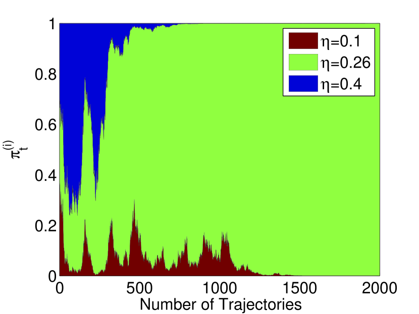
Figure 1: First estimation, with pattern values $\eta_{1}=0.10$, the parameter value $\eta_{2}=0.26$ close to $\overline{\eta}$, and $\eta_{3}=0.40$. Only the first $2000$ trajectories are needed to select $\overline{\eta}\approx 0.26$ and discard $0.10$ and $0.40$.

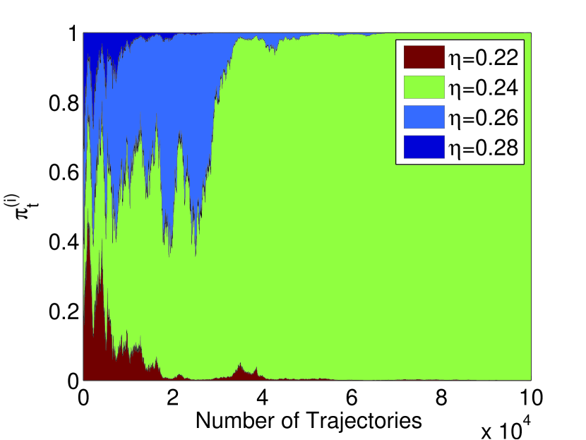
Figure 2: Second estimation, realized with more narrow intervals between each pattern values. We notice that $\overline{\eta}$ is actually closer to $0.24$ than $0.26$, the calibrated value, and that the number of trajectories required for the discrimination has drastically increased to $1\times 10^{5}$.

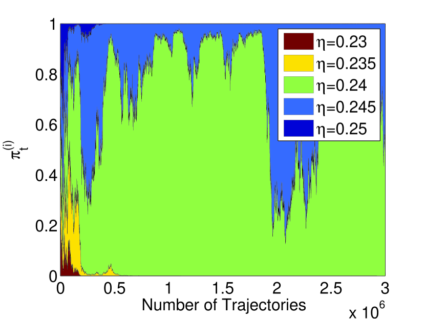
Figure 3: Last estimation, with very narrow intervals. We use all the trajectories available, i.e. $3\times 10^{6}$ trajectories. Filter does not converge to a distinct choice between $0.240$ and $0.245$.

V Conclusion

We have shown that particle quantum filtering is always a stable process. We have proposed an original positivity preserving formulation for systems governed by diffusive stochastic master equation. A first validation on experimental data confirms the interest of the resulting parameter algorithm. This positivity preserving algorithm appears to be robust enough to cope with sampling time of more than 2% of the characteristic time attached to the measurement. The convergence characterization of such estimation scheme remains to be done despite the fact they are always stable.

References

- [1] H. Amini, C. Pellegrini, and P. Rouchon. Stability of continuous-time quantum filters with measurement imperfections. Russian Journal of Mathematical Physics, 21(3):297–315–, 2014.
- [2] H. Amini, R.A. Somaraju, I. Dotsenko, C. Sayrin, M. Mirrahimi, and P. Rouchon. Feedback stabilization of discrete-time quantum systems subject to non-demolition measurements with imperfections and delays. Automatica, 49(9):2683–2692, September 2013.
- [3] A. Barchielli and M. Gregoratti. Quantum Trajectories and Measurements in Continuous Time: the Diffusive Case. Springer Verlag, 2009.
- [4] S. Brakhane, Alt W., T.Kampschulte, M. Martinez-Dorantes, R. Reimann, S. Yoon, A. Widera, and D. Meschede. Bayesian feedback control of a two-atom spin-state in an atom-cavity system. Phys. Rev. Lett., 109(17):173601–, October 2012.
- [5] P. Campagne-Ibarcq, L. Bretheau, E. Flurin, A. Auffèves, F. Mallet, and B. Huard. Observing interferences between past and future quantum states in resonance fluorescence. Phys. Rev. Lett., 112:180402, May 2014.
- [6] P. Campagne-Ibarcq et al., in preparation.
- [7] O. Cappé, E. Moulines, and T. Ryden. Inference in Hidden Markov Models. Springer series in statistics, 2005.
- [8] Bradley A. Chase and J. M. Geremia. Single-shot parameter estimation via continuous quantum measurement. Phys. Rev. A, 79(2):022314–, February 2009.
- [9] E.B. Davies. Quantum Theory of Open Systems. Academic Press, 1976.
- [10] I. Dotsenko, M. Mirrahimi, M. Brune, S. Haroche, J.-M. Raimond, and P. Rouchon. Quantum feedback by discrete quantum non-demolition measurements: towards on-demand generation of photon-number states. Physical Review A, 80: 013805-013813, 2009.
- [11] J. Gambetta and H. M. Wiseman. State and dynamical parameter estimation for open quantum systems. Phys. Rev. A, 64(4):042105–, September 2001.
- [12] S. Haroche and J.M. Raimond. Exploring the Quantum: Atoms, Cavities and Photons. Oxford University Press, 2006.
- [13] M. Hatridge et al., Quantum Back-Action of an Individual Variable-Strength Measurement. Science, 339:178 (2013)
- [14] Y. Kato and N. Yamamoto. Estimation and initialization of quantum network via continuous measurement on single node. In Decision and Control (CDC), 2013 IEEE 52nd Annual Conference on, pages 1904–1909, 2013.
- [15] H Mabuchi. Dynamical identification of open quantum systems. Quantum and Semiclassical Optics: Journal of the European Optical Society Part B, 8(6):1103–, 1996.
- [16] A Negretti and K Mølmer. Estimation of classical parameters via continuous probing of complementary quantum observables. New Journal of Physics, 15(12):125002–, 2013.
- [17] M.A. Nielsen and I.L. Chuang. Quantum Computation and Quantum Information. Cambridge University Press, 2000.
- [18] N. Roch et al., Widely Tunable, Nondegenerate Three-Wave Mixing Microwave Device Operating near the Quantum Limit Physical Review Letters, 108:147701 (2012)
- [19] P. Rouchon. Fidelity is a sub-martingale for discrete-time quantum filters. IEEE Transactions on Automatic Control, 56(11):2743–2747, 2011.
- [20] P. Rouchon and J. F. Ralph. Efficient quantum filtering for quantum feedback control. Phys. Rev. A, 91(1):012118–, January 2015.
- [21] A. Somaraju, I. Dotsenko, C. Sayrin, and P. Rouchon. Design and stability of discrete-time quantum filters with measurement imperfections. In American Control Conference, pages 5084–5089, 2012.
- [22] H.M. Wiseman and G.J. Milburn. Quantum Measurement and Control. Cambridge University Press, 2009.