Sedimentation of finite-size spheres in quiescent and turbulent environments

Abstract

Sedimentation of a dispersed solid phase is widely encountered in applications and environmental flows, yet little is known about the behavior of finite-size particles in homogeneous isotropic turbulence. To fill this gap, we perform Direct Numerical Simulations of sedimentation in quiescent and turbulent environments using an Immersed Boundary Method to account for the dispersed rigid spherical particles. The solid volume fractions considered are $\phi=0.5-1\%$, while the solid to fluid density ratio $\rho_{p}/\rho_{f}=1.02$. The particle radius is chosen to be approximately 6 Komlogorov lengthscales. The results show that the mean settling velocity is lower in an already turbulent flow than in a quiescent fluid. The reduction with respect to a single particle in quiescent fluid is about 12% and 14% for the two volume fractions investigated. The probability density function of the particle velocity is almost Gaussian in a turbulent flow, whereas it displays large positive tails in quiescent fluid. These tails are associated to the intermittent fast sedimentation of particle pairs in drafting-kissing-tumbling motions. The particle lateral dispersion is higher in a turbulent flow, whereas the vertical one is, surprisingly, of comparable magnitude as a consequence of the highly intermittent behavior observed in the quiescent fluid. Using the concept of mean relative velocity we estimate the mean drag coefficient from empirical formulas and show that non stationary effects, related to vortex shedding, explain the increased reduction in mean settling velocity in a turbulent environment.

1 Introduction

The gravity-driven motion of solid particles in a viscous fluid is a relevant process in a wide number of scientific and engineering applications (Guazzelli & Morris, 2012). Among these we recall fluvial geomorphology, chemical engineering systems, as well as pollutant transport in underground water and settling of micro-organisms such as plankton.
The general problem of sedimentation is very complex due to the high number of factors from which it depends. Sedimentation involves large numbers of particles settling in different environments. The fluid in which the particles are suspended may be quiescent or turbulent. Particles may differ in size, shape, density and stiffness. The range of spatial and temporal scales involved is wide and the global properties of these suspensions can be substantially different from one case to another. Because of these complexities, our general understanding of the problem is still incomplete.

1.1 Settling in a quiescent fluid

One of the earliest investigations on the subject at hand is Stokes’ analysis of the sedimentation of a single rigid sphere through an unbounded quiescent viscous fluid at zero Reynolds number. This led to the well-known formula that links the settling velocity to the sphere radius, the solid to fluid density ratio and the viscosity of the fluid that bears his name. Later, the problem was studied both theoretically and experimentally. Hasimoto (1959) obtained expressions for the drag force exerted by the fluid on three different cubic arrays of rigid spheres. These relate the drag force only to the solid volume fraction, but were derived under the assumption of very dilute suspensions and Stokes flow. The formulae have later been revisited by Sangani & Acrivos (1982). A different approach was instead pursued by Batchelor (1972) who found a relation between the mean settling velocity and the solid volume fraction by using conditional probability arguments. When the Reynolds number of the settling particles ($Re_{t}$) becomes finite, the assumption of Stokes flow is less acceptable (especially for $Re_{t}>1$). The fore-aft symmetry of the fluid flow around the particles is broken and wakes form behind them. Solutions should be derived using the Navier-Stokes equations, but the nonlinearity of the inertial term makes the analytical treatment of such problems extremely difficult. For this reason theoretical investigations have progressively given way to experimental and numerical approaches.
The first remarkable experimental results obtained for creeping flow were those by Richardson & Zaki (1954). These authors proposed an empirical formula relating the mean settling velocity of a suspension to its volume fraction and to the settling velocity of an isolated particle. This formula is believed to be accurate also for concentrated suspensions (up to a volume fraction $\phi$ of about $25\%$) and for low Reynolds numbers. Subsequent investigations improved the formula so that it could also be applied in the intermediate Reynolds numbers regime (Garside & Al-Dibouni, 1977; Di Felice, 1999).
Efficient algorithms and sufficient computational power have become available only relatively recently and since then many different numerical methods have been used to improve our understanding of the problem (Prosperetti, 2015). Among others we recall the dynamical simulations performed by Ladd (1993), the finite-elements simulations of Johnson & Tezduyar (1996), the force-coupling method simulations by Climent & Maxey (2003), the Lattice-Boltzmann simulations of Yin & Koch (2007), the Oseenlet simulations by Pignatel et al. (2011), and the Immersed Boundary simulations of Kempe & Fröhlich (2012) and Uhlmann & Doychev (2014). Thanks to the most recent techniques it has become feasible to gain more insight on the interactions among the different phases and the resulting microstructure of the sedimenting suspension (Yin & Koch, 2007; Uhlmann & Doychev, 2014). Uhlmann & Doychev (2014), most recently, simulated the settling of dilute suspensions with particle Reynolds numbers in the range $140-260$ and studied the effect of the Archimedes number (namely the ratio between gravitational and viscous forces) on the microscopic and macroscopic properties of the suspension. These authors observe an increase of the settling velocity at higher Archimedes, owing to particle clustering in a regime where the flow undergoes a steady bifurcation to an asymmetric wake. Settling in stratified environments has also been investigated experimentally, i.e. by Bush et al. (2003), and numerically, i.e. by Doostmohammadi & Ardekani (2015).

1.2 Sedimentation in an already turbulent flow

The investigations previously reported consider the settling of particles in quiescent or uniform flows. There are many situations though, where the ambient fluid is in fact nonuniform or turbulent. As in the previous case, the first approach to this problem was analytical. In the late 40’s and 50’s Tchen (1947) and later Corrsin & Lumley (1956) proposed an equation for the motion of a small rigid sphere settling in a nonuniform flow. In the derivation, they assumed the particle Reynolds number to be very low so that the viscous Stokes drag for a sphere could be applied. The added mass and the augmented viscous drag due to a Basset history term were also included. Maxey & Riley (1983) corrected these equations including also the Faxen forces due to the unsteady Stokes flow.
In a turbulent flow many different spatial and temporal scales are active. Therefore the behaviour and motion of one single particle does not depend only on its dimensions and characteristic response time, but also on the ratios among these and the characteristic turbulent length and time scales. The turbulent quantities usually considered are the Kolmogorov length and time scales which are related to the smallest eddies. Alternatively, the integral lengthscale and the eddy turnover time can also be used. It is clear that a particle smaller than the Kolmogorov legthscale will behave differently than a particle of size comparable to the energetic flow structures. A sufficiently large particle with a characteristic time scale larger than the timescale of the velocity fluctuations will definitely be affected by and affect the turbulence. A smaller particle with a shorter relaxation time will more closely follow the turbulent fluctuations. When particle suspensions are considered, the situation becomes even more complicated. If the particles are solid, smaller than the Kolmogorov lengthscale and dilute, the turbulent flow field is unaltered (i.e., one-way coupling). Interestingly, the turbulent dynamics is instead altered by microbubbles. The presence of these microbubbles leads to relevant drag reduction in boundary layers and shears flows (e.g. Taylor-Couette flow)(Sugiyama et al., 2008; Ceccio, 2010). If the mass of the dispersed phase is similar to that of the carrier phase, the influence of the solid phase on the fluid phase cannot be ignored (i.e., two-way coupling). Interactions among particles (such as collisions) must also be considered in concentrated suspensions. This last regime is described as four-way coupling (Elgobashi, 1991; Balachandar & Eaton, 2010).

Because of the difficulty of treating the problem analytically, the investigations of the last three decades have mostly been either experimental or numerical. In most of the numerical studies heavy and small particles were considered. The reader is referred to Toschi & Bodenschatz (2009) for a more detailed review than the short summary reported here. Wang & Maxey (1993) studied the settling of dilute heavy particles in homogeneous isotropic turbulence. The particle Reynolds number based on the relative velocity was assumed to be much less than unity so that Stokes drag force could be used to determine the particle motion. These authors show that heavy particles smaller than the Kolmogorov lengthscale tend to move outward from the center of eddies and are often swept into regions of downdrafts (the so called preferential sweeping later renamed fast-tracking). In doing so, the particle mean settling velocity is increased with respect to that in a quiescent fluid. A series of studies confirmed and extended these results examining particle clustering (Bec et al., 2014; Gustavsson et al., 2014), preferential concentration (Aliseda et al., 2002), the effects of the particle shape, orientation and collision rates (Siewert et al., 2014), as well the effects of one- or two-way coupling algorithms (Bosse et al., 2006), to mention few aspects. Numerous experimental studies were also performed in order to confirm these results and to study the turbulence modulation due to the presence of particles (Hwang & Eaton, 2006).

The results on the mean settling velocities of particles of the order or larger than the Kolmogorov scale are not conclusive. Good et al. (2014) studied particles smaller than the Kolmogorov scale and with density ratio $\mathcal{O}(1000)$, whereas Variano (experiments; private communication) and Byron (2015) studied finite-size particles at density ratios comparable to ours. Good et al. (2014) found that the mean settling velocity is reduced only when nonlinear drag corrections are considered in a one-way coupling approach when particles have a long relaxation time (a linear drag force would always lead to a settling velocity enhancement). For finite-size almost neutrally-buoyant particles, Variano and Byron (2015) observe instead that the mean settling velocity is smaller than in a quiescent fluid. In relative terms, the settling velocity decreases more and more as the ratio between the turbulence fluctuations and the terminal velocity of a single particle in a quiescent fluid increases. It is generally believed that the reduction of settling speed is due to the non-linear relation between the particle drag and the Reynolds number. Nonetheless, unsteady and history effects may also play a key role (Olivieri et al., 2014; Bergougnoux et al., 2014). Tunstall & Houghton (1968) demonstrated already in 1968 that the average settling velocity is reduced in a flow oscillating about a zero mean, due to the interactions of the particle inertia with a non-linear drag force. Stout et al. (1995) tried to motivate these findings in terms of the relative motion between the fluid and the particles. When the period of the fluid velocity fluctuations is smaller than the particle response time, a significant relative motion is generated between the two phases. Due to the drag non-linearity, appreciable upward forces can be produced on the particles thereby reducing the mean settling velocity.
Unsteady effects may become important when considering suspensions with moderate particle-fluid density ratios, as suggested by Mordant & Pinton (2000) and Sobral, Oliveira & Cunha (2007). The former studied experimentally the motion of a solid sphere settling in a quiescent fluid and explain the transitory oscillations of the settling velocity found at $Re\approx O(100)$ by the presence of a transient vortex shedding in the particle wake. The latter, instead, analyzed an equation similar to that proposed by Maxey & Riley (1983), and suggested that unsteady hydrodynamic drags might become important when the density ratio approaches unity.

1.3 Fully resolved simulations

As already mentioned, most of the numerical studies of settling in turbulent flows used either one or two-way coupling algorithms. In order to properly understand the microscopical phenomena at play, it would be ideal to use fully resolved simulations. An algorithm often used to accomplish this is the Immersed Boundary Method with direct forcing for the simulation of particulate flows originally developed by Uhlmann (2005). The code was later used to study the clustering of non-colloidal particles settling in a quiescent environment (Uhlmann & Doychev, 2014). With a similar method Lucci et al. (2010) studied the modulation of isotropic turbulence by particles of Taylor length-scale size. Recently, Homann et al. (2013) used an Immersed Boundary Fourier-spectral method to study finite-size effects on the dynamics of single particles in turbulent flows. These authors found that the drag force on a particle suspended in a turbulent flow increases as a function of the turbulent intensity and the particle Reynolds number. We recently used a similar algorithm to examine turbulent channel flows of particle suspensions (Picano, Breugem & Brandt, 2015).

The aim of the present study is to simulate the sedimentation of a suspension of particles larger than the Kolmogorov lengthscale in homogeneous isotropic turbulence with a finite difference Immersed Boundary Method. We focus on particles slightly denser than the suspending fluid ($\rho_{p}/\rho_{f}=1.02$) and investigate particle and fluid velocity statistics, non-linear and unsteady contributions to the overall drag and turbulence modulation. The suspensions considered in this work are dilute ($\phi=0.5-1\%$) and monodispersed. The same simulations are also performed in absence of turbulence to appreciate differences of the particle velocity statistics in the two different environments. Due to the size of the particles considered it has been necessary to consider very long computational domains in the settling direction, especially for the quiescent environment. In the turbulent cases, smaller domains provide converged statistics since the particle wakes are disrupted faster. The parameters of the simulations have been inspired by the experiments by Variano, Byron (2015) and co-workers at UC Berkeley. These authors investigate Taylor-scale particles in turbulent aquatic environments using Refractive-Index-Matched Hydrogel particles to measure particle linear and angular velocities.

Our results show that the mean settling velocity is lower in an already turbulent flow than in a quiescent fluid. The reduction is about $12\%$ and $14\%$ for the two volume fractions investigated. By looking at probability density functions $pdf$ of the settling velocities, we observe that the $pdf$ is well approximated by a Gaussian function centered around the mean in the turbulent cases. In the laminar case instead, the $pdf$ shows a smaller variance and a larger skewness, indicating that it is more probable to find particles settling more rapidly than the mean value rather than more slowly. These events are associated to particle-particle interactions, in particular to the drifting-kissing-tumbling motion of particle pairs. We also calculate mean relative velocity fields and notice that vortex shedding occurs around each particle in a turbulent environment. Using the concept of mean relative velocity we calculate a local Reynolds number and the mean drag coefficient from empirical formulas to quantify the importance of unsteady and history effects on the overall drag, thereby explaining the reduction in mean settling velocity. In fact, these terms become important only in a turbulent environment.

2 Methodology

2.1 Numerical Algorithm

Different methods have been proposed in the last years to perform Direct Numerical Simulations of multiphase flows. The Lagrangian-Eulerian algorithms are believed to be the most appropriate for solid-fluid suspensions (Ladd & Verberg, 2001; Zhang & Prosperetti, 2010; Lucci et al., 2010; Uhlmann & Doychev, 2014). In the present study, simulations have been performed using a tri-periodic version of the numerical code originally developed by Breugem (2012) that models the coupling between the solid and fluid phases. The Eulerian fluid phase is evolved according to the incompressible Navier-Stokes equations,

$${\bf\nabla\cdot}{\bf u}_{f}=0$$ (1)

$$\frac{\partial{\bf u}_{f}}{\partial t}+{\bf u}_{f}\cdot{\bf\nabla}{\bf u}_{f}=-\frac{1}{\rho_{f}}{\bf\nabla}p+\nu{\bf\nabla}^{2}{\bf u}_{f}+{\bf f}$$ (2)

where ${\bf u}_{f}$, $\rho_{f}$ and $\nu=\mu/\rho_{f}$ are the fluid velocity, density and kinematic viscosity respectively ($\mu$ is the dynamic viscosity), while $p$ and ${\bf f}$ are the pressure and the force field used to mantain turbulence and model the presence of particles. The particles centroid linear and angular velocities, ${\bf u}_{p}$ and ${\bf\boldsymbol{\omega}}_{p}$ are instead governed by the Newton-Euler Lagrangian equations,

$$\rho_{p}V_{p}\frac{d{\bf u}_{p}}{dt} =\rho_{f}\oint_{\partial\mathcal{V}_{p}}{\bf\boldsymbol{\tau}}\cdot{\bf n}\,dS+\left(\rho_{p}-\rho_{f}\right)V_{p}{\bf g}$$ (3)

$$I_{p}\frac{d{\bf\boldsymbol{\omega}}_{p}}{dt} =\rho_{f}\oint_{\partial\mathcal{V}_{p}}{\bf r}\times{\bf\boldsymbol{\tau}}\cdot{\bf n}\,dS$$ (4)

where $V_{p}=4\pi a^{3}/3$ and $I_{p}=2\rho_{p}V_{p}a^{2}/5$ are the particle volume and moment of inertia, with $a$ the particle radius; ${\bf g}$ is the gravitational acceleration; ${\bf\boldsymbol{\tau}}=-p{\bf I}+2\mu{\bf E}$ is the fluid stress, with ${\bf I}$ the identity matrix and ${\bf E}=\left({\bf\nabla}{\bf u}_{f}+{\bf\nabla}{\bf u}_{f}^{T}\right)/2$ the deformation tensor; ${\bf r}$ is the distance vector from the center of the sphere while $\bf{n}$ is the unit vector normal to the particle surface $\partial\mathcal{V}_{p}$. Dirichlet boundary conditions for the fluid phase are enforced on the particle surfaces as ${\bf u}_{f}|_{\partial\mathcal{V}_{p}}={\bf u}_{p}+{\bf\boldsymbol{\omega}}_{p}\times{\bf r}$.
In the numerical code the coupling between the solid and fluid phases is obtained by using an Immersed Boundary Method. The boundary condition at the moving particle surface (i.e. ${\bf u}_{f}|_{\partial\mathcal{V}_{p}}={\bf u}_{p}+{\bf\boldsymbol{\omega}}_{p}\times{\bf r}$) is modeled by adding a force field on the right-hand side of the Navier-Stokes equations. The problem of re-meshing is therefore avoided and the fluid phase is evolved in the whole computational domain using a second order finite difference scheme on a staggered mesh. The time integration is performed by a third order Runge-Kutta scheme combined with a pressure-correction method at each sub-step. The same integration scheme is also used for the Lagrangian evolution of eqs. (3) and (4). The forces exchanged by the fluid and the particles are imposed on $N_{L}$ Lagrangian points uniformly distributed on the particle surface. The force ${\bf F}_{l}$ acting on the $l-th$ Lagrangian point is related to the Eulerian force field ${\bf f}$ by the expression ${\bf f}({\bf x})=\sum_{l=1}^{N_{L}}{\bf F}_{l}\delta_{d}({\bf x}-{\bf X}_{l})\Delta V_{l}$. In the latter $\Delta V_{l}$ represents the volume of the cell containing the $l-th$ Lagrangian point while $\delta_{d}$ is the Dirac delta. This force field is obtained through an iterative algorithm that mantains second order global accuracy in space. Using this IBM force field eqs. (3) and  (4) are rearranged as follows to maintain accuracy,

$$\rho_{p}V_{p}\frac{d{\bf u}_{p}}{dt} =-\rho_{f}\sum_{l=1}^{N_{l}}{\bf F}_{l}\Delta V_{l}+\rho_{f}\frac{d}{dt}\int_{\mathcal{V}_{p}}{\bf u}_{f}\,dV+\left(\rho_{p}-\rho_{f}\right)V_{p}{\bf g}$$ (5)

$$I_{p}\frac{d{\bf\boldsymbol{\omega}}_{p}}{dt} =-\rho_{f}\sum_{l=1}^{N_{l}}{\bf r}_{l}\times{\bf F}_{l}\Delta V_{l}+\rho_{f}\frac{d}{dt}\int_{\mathcal{V}_{p}}{\bf r}\times{\bf u}_{f}\,dV$$ (6)

where the second terms on the right-hand sides are corrections to account for the inertia of the fictitious fluid contained within the particle volume. In eqs. (5),(6) ${\bf r}_{l}$ is simply the distance from the center of a particle. Particle-particle interactions are also considered. When the gap distance between two particles is smaller than twice the mesh size, lubrication models based on Brenner’s asymptotic solution (Brenner, 1961) are used to correctly reproduce the interaction between the particles. A soft-collision model is used to account for collisions among particles with an almost elastic rebound (the restitution coefficient is $0.97$). These lubrication and collision forces are added to the right-hand side of eq. (5). More details and validations of the numerical code can be found in Breugem (2012), Lambert et al. (2013), Lashgari et al. (2014) and Picano et al. (2015).

2.2 Parameter setting

Sedimentation of dilute particle suspensions is considered in an unbounded computational domain with periodic boundary conditions in the $x$, $y$ and $z$ directions. Gravity is chosen to act in the positive $z$ direction. A zero mass flux is imposed in the simulations. A cubic mesh is used to discretise the computational domain with eight points per particle radius, $a$. Non-Brownian rigid spheres are considered with solid to fluid density ratio $\rho_{p}/\rho_{f}=1.02$. Hence, we consider particles slightly heavier than the suspending fluid. Two different solid volume fractions $\phi=0.5\%$ and $1\%$ are considered. In addition to the solid to fluid density ratio $\rho_{p}/\rho_{f}$ and the solid volume fraction $\phi$, it is necessary to introduce another nondimensional number. This is the Archimedes number (or alternatively the Galileo number $Ga=\sqrt{Ar}$),

$$Ar=\frac{\left(\frac{\rho_{p}}{\rho_{f}}-1\right)g(2a)^{3}}{\nu^{2}}$$ (7)

a nondimensional number that quantifies the importance of the gravitational forces acting on the particle with respect to viscous forces. In the present case the Archimedes number $Ar=21000$. Using the particle terminal velocity $v_{t}$ we define the Reynolds number $Re_{t}=2av_{t}/\nu$. This can be related by empirical relations to the drag coefficient of an isolated sphere when varying the Archimedes number, $Ar$. Different versions of these empirical relations giving the drag coefficient as a function of $Re_{t}$ and $Ar$ have been proposed. As Yin & Koch (2007) we will use the following relations,

$$C_{D}=\left\{\begin{array}[]{ll}\frac{24}{Re_{t}}\left[1+0.1315Re_{t}^{(0.82-0.05log_{10}Re_{t})}\right],&0.01<Re_{t}\leq 20\\[2.0pt] \frac{24}{Re_{t}}\left[1+0.1935Re_{t}^{0.6305}\right],&20<Re_{t}<260\end{array}\right.$$ (8)

since $C_{D}={4}{Ar}/(3{Re_{t}^{2}})$ (Yin & Koch, 2007) we finally write,

$$Ar=\left\{\begin{array}[]{ll}18Re_{t}\left[1+0.1315Re_{t}^{(0.82-0.05log_{10}Re_{t})}\right],&0.01<Re_{t}\leq 20\\[2.0pt] 18Re_{t}\left[1+0.1935Re_{t}^{0.6305}\right],&20<Re_{t}<260\end{array}\right.$$ (9)

The Reynolds number calculated from eq. (9) is approximately $188$ for $Ar=21000$.

In order to generate and sustain an isotropic and homogeneous turbulent flow field, a random forcing is applied to the first shell of wave vectors. We consider a $\delta$-correlated in time forcing of fixed amplitude $\hat{f}_{0}$ (Vincent & Meneguzzi, 1991; Zhan et al., 2014). The turbulent field, alone, is characterized by a Reynolds number based on the Taylor microscale, $Re_{\lambda}=\lambda u^{\prime}/\nu$, where $u^{\prime}$ is the fluctuating velocity and $\lambda=\sqrt{15\nu u^{\prime 2}/\epsilon}$ is the transverse Taylor length scale. This is about $90$ in our simulations. The ratio between the grid spacing and the Kolmogorov lengthscale $\eta=(\nu^{3}/\epsilon)^{1/4}$ (where $\epsilon$ is the energy dissipation) is approximately $1.3$ while the particle diameter is circa $12\eta$. Finally, the ratio among the expected mean settling velocity and the turbulent velocity fluctuations is $v_{t}/u^{\prime}=3.4$. The parameters of the turbulent flow field are summarized in table 1. For the definition of these parameters, the reader is referred to Pope (2000).

2.3 Validation

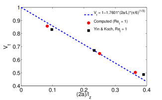
Figure 1: Terminal velocity of a periodic array of spheres. Present results $Re_{t}=1$ denoted by red circles are compared with the ones obtained by Yin and Koch by black squares at the same $Re_{t}$ and with the analytical solution for $Re_{t}=0$ of eq. (10).

To check the validity of our approach we performed simulations of a single sphere settling in a cubic lattice in boxes of different sizes. Since this is equivalent to changing the solid volume fraction, we compared our results to the analytical formula derived by Hasimoto (1959) and Sangani & Acrivos (1982),

$$|{\bf V}_{t}|=\frac{|{\bf v}_{t}|}{|{\bf V}_{s}|}=1-1.7601\phi^{1/3}$$ (10)

where

$$|{\bf V}_{s}|=\frac{2}{9}\frac{\left(\frac{\rho_{p}}{\rho_{f}}-1\right)ga^{2}}{\nu}$$ (11)

is the Stokes settling velocity. In terms of the size of the computational domain, $l_{z}$, eq. (10) can also be rewritten as $V_{t}=1-1.7601(2a/l_{z})(\pi/6)^{1/3}$. In figure 1 we show the results obtained with our code for $Re_{t}=1$ together with the data by Yin & Koch (2007) and the analytical solution. Although the analytical solution was derived with the assumption of vanishing Reynolds numbers, we find good agreement among the various results.

The actual problem arises when considering particles settling at relatively high Reynolds numbers. If the computational box is not sufficiently long in the gravity direction, a particle would fall inside its own wake (due to periodic boundary conditions), thereby accelerating unrealistically. Various simulations of a single particle falling in boxes of different size were preliminarily carried out, in particular $48a\times 48a\times 48a$, $32a\times 32a\times 96a$ and $32a\times 32a\times 320a$. The first two boxes turn out to be unsuitable for our purposes. We find a terminal Reynolds number $Re_{t}=200$ in the longest domain considered, which corresponds to a difference of about 6% with respect to the value obtained from the empirical relations (9). As reference velocity we use the value obtained from simulations performed in the largest box at a solid volume fraction two orders of magnitude smaller than the cases under investigation, $\phi=5\cdot 10^{-5}$ (as in Uhlmann & Doychev, 2014), corresponding to a terminal velocity such that $Re_{t}=195$, 4% larger than the value from the empirical relations (9). Further increasing the length in the $z$ direction would make the simulations prohibitive. Note also that simulations in a turbulent environment turn out to be less demanding as turbulence disrupts and decorrelates the flow structures induced by the particles. The final choice was therefore a computational box of size $32a\times 32a\times 320a$ with $256\times 256\times 2560$ grid points, $391$ particles for $\phi=0.5\%$ and $782$ particles for $\phi=1\%$. In all cases, the particles are initially distributed randomly in the computational volume with zero initial velocity and rotation.

$\eta/(2a)$	$u^{\prime}$	$k$	$\lambda/(2a)$	$Re_{\lambda}$	$\epsilon$	$T_{e}$	$Re_{L_{0}}$
0.084	0.30	0.13	1.56	90	0.0028	46.86	1205

Table 1: Turbulent flow parameters in particle units, where $k$ is the turbulent kinetic energy, $\lambda$ is the Taylor microscale, $T_{e}=k/\epsilon$ is the eddy turnover time and $Re_{L_{0}}$ is the Reynolds number based on the integral lengthscale $L_{0}=k^{3/2}/\epsilon$.

A snapshot of the suspension flow for $\phi=0.5\%$ is shown in figure 2. The instantaneous velocity component perpendicular to gravity is shown on different orthogonal planes.

The simulations were run on a Cray XE6 system at the PDC Center for High Performance Computing at the KTH, Royal Institue of Technology. The fluid phase is evolved for approximately $6$ eddy turnover times before adding the solid phase. The simulations for each solid volume fraction were performed for both quiescent fluid and turbulent flow cases in order to compare the results. Statistics are collected after an initial transient phase of about $4$ eddy turnover times for the turbulent case and $15$ relaxation times ($T_{p}=2\rho_{p}a^{2}/(9\rho_{f}\nu)$) for the quiescent case. Defining as reference time the time it takes for an isolated particle to fall over a distance equal to its diameter, $2a/v_{t}$, the initial transient corresponds to approximately $170$ units. Statistics are collected over a time interval of 500 and 300 in units of $2a/v_{t}$ for the quiescent and turbulent cases, respectively. Differences between the statistics presented here and those computed from half the samples is below 1% for the first and second moments.

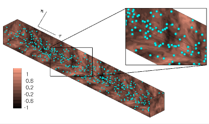
Figure 2: Instantaneous snapshot of the velocity component perpendicular to gravity on different orthogonal planes, together with the corresponding particle position for $\phi=0.005$. A zoomed view of a particular section is also shown.

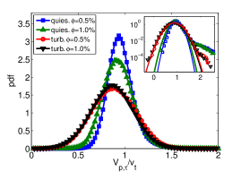
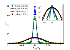
Figure 3: Probability density functions of the particles velocities along the directions a) parallel $V_{p,\tau}$ and b) perpendicular $V_{p,n}$ to gravity for $\phi=0.5\%$ and $1\%$. The velocities are normalized by $v_{t}$. Quiescent fluid cases denoted by blue curve with squares for $\phi=0.5\%$ and green curve with triangles for $\phi=1\%$, turbulent flow data by red curve with circles for $\phi=0.5\%$ and black curve with downward-pointing triangles for $\phi=1\%$. In the insets we show the $pdf$s in lin-log scale.

3 Results

We investigate and compare the behavior of a suspension of buoyant particles in a quiescent and turbulent environment. The behaviour of a suspension in a turbulent flow depends on both the particles and turbulence characteristic time- and length-scales: homogeneous and isotropic turbulence is defined by the dissipative, Taylor and integral scales, whereas the particles are characterized by their settling velocity $v_{t}$ and by their Stokesian relaxation time $T_{p}=2\rho_{p}a^{2}/(9\rho_{f}\nu)=11.1$ (time is scaled by $(2a/v_{t})$ throughout the paper). A comparison between characteristic time scales is given by the Stokes number, i.e. the ratio between the particle relaxation time and a typical flow time scale $St_{f}=T_{p}/T_{f}$. In the present cases, the Stokes number based on the dissipative scales (time and velocity) is $St_{\eta}=T_{p}/T_{K}=8.1$ so the particles are inertial on this scale. In addition, because the particles are about 12 times larger than the Kolmogorov length and fall about 16 times faster than the Kolmogorov velocity scale, we can expect that motions at the smallest scales weakly affect the particle dynamics.

Considering therefore the large-scale motions, we introduce an integral-scale Stokes number $St_{T_{e}}=T_{p}/T_{e}=0.24$. This value of $St_{T_{e}}$ reflects the fact that the particles are about 20 times smaller than the integral length scale $L_{0}$. The strong coupling between particle dynamics and turbulent flow field occurs at scales of the order of the Taylor scale for the present cases. Indeed, the Taylor Stokes number is $St_{\lambda}=T_{p}/T_{\lambda}=2.1$ with $T_{\lambda}=\lambda/u^{\prime}$. It should be noted that the Taylor length is slightly larger than the particle size, $3.1a$, while particles fall around 3.4 times faster than typical fluid velocity fluctuations, $v_{t}/u^{\prime}=3.4$. Hence particles are strongly influenced by the fluid fluctuations occurring at scales of the order of $\lambda$.

3.1 Particle statistics

We start by comparing the single-point flow and particle velocity statistics for the two cases studied, i.e. quiescent and turbulent flow. The results are collected when a statistically steady state is reached. Due to the axial symmetry with respect to the direction of gravity, we consider only two velocity components for both phases, the components parallel and perpendicular to gravity, $V_{\alpha,\tau}$ and $V_{\alpha,n}$ respectively, where $\alpha=f,\,p$ indicates the solid and fluid phases.

In figure 3 we report the probability density function of the particle velocities for both volume fraction investigated here, $\phi=0.5\%$ and $1\%$; the moments extracted from these distribution are summarized in table 2. The data in 3a) show the $pdf$ for the component of the velocity aligned with gravity $V_{p,\tau}$ normalized by the settling velocity for $\phi\to 0$ in a quiescent environment, $v_{t}$. This is extracted from the simulation of a very dilute suspension discussed in section 2.3.

In the quiescent cases, the mean settling velocity slightly reduces when increasing the volume fraction $\phi$, in agreement with the findings of Richardson & Zaki (1954) and Di Felice (1999) among others. The sedimentation velocity decreases to 0.96 at $\phi=0.5\%$ and 0.93 at $\phi=1\%$. Di Felice (1999) investigated experimentally the settling velocity of dilute suspensions of spheres ($\phi=0.5\%$) with density ratio 1.2 in quiescent fluid, for a large range of terminal Reynolds numbers (from $0.01$ to $1000$). Following the empirical fit proposed in Di Felice (1999), we obtain $\langle V_{f,\tau}\rangle\simeq 0.98$ at $\phi=0.5\%$, approximately $1\%$ larger than our result. On the other hand, the formula suggested for the intermediate regime in Di Felice (1999) and Yin & Koch (2007), $Re_{t}<150$, would give an estimated value of 0.88, $6\%$ lower than our result.

The mean settling velocity for the quiescent case at $\phi=0.5\%$ is instead close to the estimated value from eq. (9). This is in agreement with what reported in Uhlmann & Doychev (2014). These authors found that the particle mean settling velocity of a dilute suspension increases above the reference value only when the Archimedes number $Ar$ is larger than approximately $24000$ and clustering occurs. In our case $Ar\simeq 21000$ and no clustering is noticed accordingly with their findings.

Interestingly, we observe an additional non-negligible reduction when a turbulent background flow is considered, in our opinion the main result of the paper. The reduction of the mean settling velocity $\langle V_{p,\tau}\rangle$ is $12\%$ at $\phi=0.5\%$ and $14\%$ at $\phi=1\%$, see table 2. This result unequivocally shows that the turbulence reduces the settling velocity of a suspension of finite-size buoyant particles, in agreement with the experimental findings by Variano and co-workers (Variano, private communication) and Byron (2015). We also note that the reduction of the settling velocity with the volume fraction is less important for the turbulent cases.

Looking more carefully at the $pdf$s we note that fluctuations are, as expected, larger in a turbulent environment. In addition, the vertical particle velocity fluctuations are the largest component in a quiescent fluid, whereas in a turbulent flow the fluctuations are largest in the horizontal directions, as summarized in table 2. In the quiescent case the rms of the tangential velocity $\sigma_{V_{p,\tau}}$ is 0.15 and 0.17 for $\phi=0.5\%$ and $\phi=1\%$ respectively, while it increases up to $0.23$ in the corresponding turbulent cases. The difference in the width of the $pdf$ is particularly large in the directions normal to gravity where the rms of the variance $\sigma_{V_{p,n}}$ is 0.3 for both turbulent cases, while it is 5 and 4 times smaller for the quiescent flows at $\phi=0.5\%$ and $\phi=1\%$. We believe that the interactions among the particle wakes, mainly occurring in the settling direction, promote the higher vertical velocity fluctuations found in the quiescent cases. The shape of the $pdf$ is essentially Gaussian for the turbulent cases, showing vanishing skewness and normal flatness. Interestingly an intermittent and skewed behaviour is exhibited in the quiescent cases. The flatness $K$ is around $9$ for both components at $\phi=0.5\%$ and slightly reduces to $5.5$ at $\phi=1\%$. The settling velocity of the quiescent cases is skewed towards intense fluctuations in the direction of the gravity. The skewness $S$ is higher for the more dilute case, being $1.26$ at $\phi=0.5\%$ and $0.7$ at $\phi=1\%$.

We interpret the intermittent behavior suggested by values of $K>3$ by the collective dynamics of the particle suspension. The significant tails of the $pdf$s shown in figure 3a) are indeed associated to a specific behavior: as particles fall, they tend to be accelerated by the wakes of other particles, before showing drafting-kissing-tumbling behavior (Fortes et al., 1987). Snapshots of the drafting-kissing-tumbling behavior between two spherical particles are shown in figure 4. When this close interaction occurs, particles are found to fall with velocities that can be more than twice the mean settling velocity $\langle V_{p,\tau}\rangle$. In the quiescent case the fluid is still, the wakes are the only perturbation present in the field and are long and intense so their effect can be felt far away from the reference particle. The more dilute the suspension the more intermittent the particle velocities are. On the contrary, when the flow is turbulent the wakes are disrupted quickly and therefore fewer particles feel the presence of a wake. The velocity disturbances are now mainly due to turbulent eddies of different size that interact with the particles to increase the variance of the velocity homogeneously along all directions leading to the almost perfect normal distributions shown above, with variances similar to those of the turbulent fluctuations. The features of the particle wakes will be further discussed in this manuscript to support the present explanation.

We also note that the sedimenting speed in the quiescent fluid is determined by two opposite contributions. The excluded volume effect that contributes to a reduction of the mean settling velocity with respect to an isolated sphere and the pairwise interactions (the drafting-kissing-tumbling), increasing the mean velocity of the two particles involved in the encounter. To try to identify the importance of the drafting-kissing-tumbling effect, we fit the left part (where no intermittent behaviour is found) of the $pdf$ pertaining the quiescent case at $\phi=0.5\%$ with a gaussian function. The mean of $V_{p,\tau}$ is reduced to about $0.93$ (value due only to the hindrance effect) instead of 0.96 in the full simulation; thereby the increment in mean settling velocity due to drafting-kissing-tumbling can be estimated to be of about $3\%$.

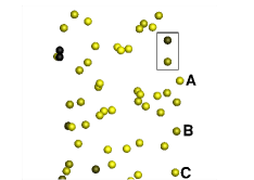
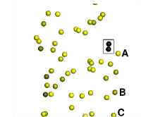
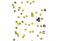
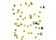
Figure 4: Drafting-kissing-tumbling behavior among two spherical particles in the quiescent case with $\phi=0.5\%$. The particles are coloured with the absolute value of their velocity component in the direction of gravity. Three particles are labeled with ”A,B,C” in order to show how accelerated the two interacting particles are compared to the others.

	Quiescent $\phi=0.5\%$	Turbulent $\phi=0.5\%$	Quiescent $\phi=1\%$	Turbulent $\phi=1\%$
$\langle V_{p,\tau}\rangle$	$+0.96$	$+0.88$	$+0.93$	$+0.86$
$\sigma_{V_{p,\tau}}$	$+0.15$	$+0.23$	$+0.17$	$+0.23$
$S_{V_{p,\tau}}$	$+1.26$	$+0.01$	$+0.70$	$+0.01$
$K_{V_{p,\tau}}$	$+9.65$	$+2.92$	$+6.01$	$+3.15$
$\langle V_{p,n}\rangle$	$+0.33\cdot 10^{-4}$	$-1.93\cdot 10^{-3}$	$-8.78\cdot 10^{-4}$	$-0.97\cdot 10^{-3}$
$\sigma_{V_{p,n}}$	$+0.06$	$+0.31$	$+0.08$	$+0.31$
$S_{V_{p,n}}$	$-1.22\cdot 10^{-3}$	$+0.04$	$-3.17\cdot 10^{-3}$	$+0.07$
$K_{V_{p,n}}$	$+8.95$	$+2.78$	$+5.55$	$+2.80$

Table 2: First four central moments of the probability density functions of $V_{p,\tau}$ and $V_{p,n}$ normalized by $v_{t}$. $S_{V_{p,\tau}}$ ($S_{V_{p,n}}$) and $K_{V_{p,\tau}}$ ($K_{V_{p,n}}$) are respectively the skewness and the flatness of the $pdf$s.

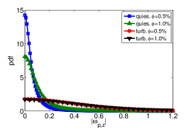
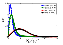
Figure 5: Probability density functions of a) $|\omega_{p,z}|$ and b) $\sqrt{\omega_{p,x}^{2}+\omega_{p,y}^{2}}$ for $\phi=0.5\%$ and $1\%$. The angular velocities are normalized by $v_{t}/(2a)$, the settling velocity of a single particle in a quiescent environment and its diameter. Quiescent fluid cases denoted by blue curve with squares for $\phi=0.5\%$ and green curve with triangles for $\phi=1\%$, turbulent flow data by red curve with circles for $\phi=0.5\%$ and black curve with downward-pointing triangles for $\phi=1\%$.

The probability density function of the particle angular velocities are also different in quiescent and turbulent flows. These are shown in figures 5a) and b) for rotations about an axis parallel to gravity, $|\omega_{p,\tau}|=|\omega_{p,z}|$, and orthogonal to it, $\sqrt{\omega_{x}^{2}+\omega_{y}^{2}}$. In the settling direction the peak of the $pdf$ is always at $|\omega_{p,z}|=0$. As for the translational velocities, the $pdf$s are broader in the turbulent cases. Due to the interaction with turbulent eddies, particles tend also to spin faster around axis perpendicular to gravity. From figure 5b) we see that the modal value slightly increases in the quiescent cases when increasing the volume fraction. In the turbulent cases, the modal value is more than $3$ times the values of the quiescent cases and the variance is also increased. Unlike the quiescent cases, the curves almost perfectly overlap for the two different $\phi$, meaning that turbulent fluctuations dominate the particle dynamics. Turbulence hinders particle hydrodynamic interactions.

Figure 6 shows the temporal correlations of the particle velocity fluctuations,

$$R_{v_{\tau}v_{\tau}}(\Delta t)=\frac{\langle V_{p,\tau}^{\prime}(p,t)V_{p,\tau}^{\prime}(p,t+\Delta t)\rangle}{\sigma_{V_{p,\tau}}^{2}}$$ (12)

$$R_{v_{n}v_{n}}(\Delta t)=\frac{\langle V_{p,n}^{\prime}(p,t)V_{p,n}^{\prime}(p,t+\Delta t)\rangle}{\sigma_{V_{p,n}}^{2}}$$ (13)

for the turbulent and quiescent cases at $\phi=0.5\%$ and $\phi=1\%$. Focusing on the data at the lower volume fraction, we observe that the particle settling velocity decorrelates much faster in the turbulent environment, within $\Delta t\sim 50$, while it takes around one order of magnitude longer in a quiescent fluid. Falling particles may encounter intense vortical structures that change their settling velocity. The turbulence strongly alters the fluid velocity field seen by the particles, which in the quiescent environment is only constituted by coherent long particle wakes. This results in a faster decorrelation of the velocity fluctuations along the settling direction in the turbulent environment. Moreover, $R_{v_{n}v_{n}}$ crosses the null value earlier than for the settling velocity component. This result is not surprising since the particle wakes develop only in the settling direction.

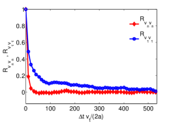
Figure 6: Time correlations of the particle velocity fluctuations. The blue curve with circles represents the correlation of $V_{p,\tau}^{\prime}$ ($R_{v_{\tau}v_{\tau}}$), while the red curve with diamonds is used for the correlation of $V_{p,n}^{\prime}$ ($R_{v_{n}v_{n}}$). a) Quiescent case with $\phi=0.5\%$, b) Turbulent case with $\phi=0.5\%$, c) Quiescent case with $\phi=1.0\%$ and d) Turbulent case with $\phi=1.0\%$.

The normal velocity correlation $R_{v_{n}v_{n}}$ of the turbulent case oscillates around zero before vanishing at longer times. We attribute this to the presence of the large-scale turbulent eddies. As a settling particle encounters sufficiently strong and large eddies, its trajectory is swept on planes normal to gravity in an oscillatory way. To provide an approximate estimate of this effect, we consider as a first approximation the turbulent flow seen by the particles as frozen since the particles fall at a higher velocity than the turbulent fluctuations (3.4 times). Since the strongest eddies are of the order of the transversal integral scale we can presume that these structures are responsible for this behavior. In particular, the transversal integral scale $L_{T}=L_{0}/2\simeq 8$ and $u^{\prime}_{rms}=0.3$, so we expect a typical period of $t=L_{T}/u^{\prime}_{rms}\simeq 26$ which is of the order of the oscillations found for both turbulent cases, i.e. $t\approx 20$. Note that a similar behavior has been observed by Wang & Maxey (1993) for sufficiently small and heavy particles, termed the preferential sweeping phenomenon.

The same process can be interpreted in terms of crossing trajectories and continuity effects as described by Csanady (1963). An inertial particle falling in a turbulent environment changes continuously its fluid-particle neighborhood. It will fall out from the eddy where it was at an earlier instant and will therefore rapidly decorrelate from the flow. In order to accommodate the back-flow necessary to satisfy continuity, the normal correlations must then contain negative loops (as those seen in figures 6b and d). Following Csanady (1963) we define the period of oscillation of the fluctuations as the ratio of the typical eddy diameter in the direction of gravity (i.e. the longitudinal integral scale $L_{0}$), and the particle terminal velocity $v_{t}$ obtaining $t=L_{0}/v_{t}\simeq 16$. This value is similar to the period of oscillations in the correlations in figure 6.

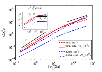
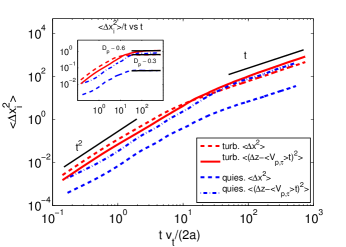
Figure 7: Mean square particle displacement in the directions parallel and perpendicular to gravity for both quiescent and turbulent cases for a) $\phi=0.5\%$ and b) $\phi=1\%$. The mean particle displacement $\langle V_{p,\tau}\rangle t$ in the settling direction is subtracted from the instantaneous displacement when computing the statistics. In the inset, we show $\langle\Delta x_{i}^{2}\rangle/t$ as a function of time as well as the diffusion coefficients $D_{e}$ for the turbulent cases.

As shown in figure 6c), the quiescent environment presents a peculiar behavior of the settling velocity correlation at $\phi=1\%$. In particular we observe oscillations around zero of long period, $T=160-180$. From the analysis of particle snapshots at different times (not shown), we observe that these seem correlated to the formation of regions of different density of the particle concentration. Hence a particle crossing regions with different local particle concentration may experience a varying settling velocity.

To further understand the particle dynamics, we display in figure 7a) and b) the single particle dispersion, i.e. the mean square displacement, for both quiescent and turbulent cases at $\phi=0.5\%$ and $1.0\%$. The mean displacement, $\langle V_{p,\tau}\rangle t$, is subtracted from the instantaneous displacement in the settling direction $\Delta z(t)$ to highlight the fluctuations with respect to the mean motion. For all cases we found initially a quadratic scaling in time ($\langle\Delta x_{i}^{2}\rangle\sim t^{2}$) typical of correlated motions while the linear diffusive behavior takes over at longer times ($\langle\Delta x_{i}^{2}\rangle\sim 2D_{e}t$ with $D_{e}$ the diffusion coefficient).

The turbulent cases show a similar behavior for both volume fractions. The crossover time when the initial quadratic scaling is lost and the linear one takes place is about $t\simeq 10$ and $t\simeq 50$ for the normal and tangential component, respectively. This difference is consistent with the correlation timescales previously discussed. The dispersion rates are similar in all directions in a turbulent environment. The quiescent cases present different features. First of all, dispersion is much more effective in the settling direction than in the normal one. The dispersion rate is smaller than the turbulent cases in the horizontal directions, while, surprisingly, the mean square displacement in the settling direction is similar to that of the turbulent cases being even higher at $\phi=0.5\%$, something we relate to the drafting-kissing-tumbling behaviour discussed above. The crossover time scale is similar to that of turbulent cases with the exception of the most dilute case which does not reach a fully diffusive behavior at $t\simeq 500$. This long correlation time makes the mean square displacement of this case higher than the corresponding turbulent case at long times.
In the insets of figure 7a) and b) we show $\langle\Delta x_{i}^{2}\rangle/t$ as a function of time. In all cases except the quiescent one at $\phi=0.5\%$, the diffusive regime is reached and it is possible to calculate the diffusion coefficients $D_{e}=\langle\Delta x_{i}^{2}\rangle/(2t)$. For the turbulent case with $\phi=0.5\%$ we obtain $D_{e}=0.52$ and $0.28$ in the directions parallel and perpendicular to gravity while for $\phi=1\%$ we obtain $D_{e}=0.57$ and $0.32$. In the quiescent cases the diffusion coefficients in the horizontal directions are approximately $0.03$, whereas the coefficient in the gravity direction at $\phi=1\%$ is about $0.40$. Csanady (1963) proposed a theoretical estimate of the diffusion coefficients for pointwise particles. Using these estimates, we obtain approximately $D_{e}=1.4$ and $0.7$ in the directions parallel and perpendicular to gravity. These are about $2.5$ times larger than those found here for finite-size particles.

3.2 Fluid statistics

Table 3 reports the fluctuation intensities of the fluid velocities for all cases considered. These are calculated by excluding the volume occupied by the spheres at each time step and averaging over the number of samples associated with the fluid phase volume. As expected, the fluid velocity fluctuations are smaller in the quiescent cases than in the turbulent regime. In the quiescent case the rms of the velocity fluctuations is about $50\%$ larger in the settling direction than in the normal direction because of the long range disturbance induced by the particles wakes. The increase of the volume fraction enhances the fluctuations in both directions. Fluctuations are always larger in the turbulent case, with the most significant differences compared to the quiescent cases in the normal direction, where the presence of the buoyant solid phase brakes the isotropy of the turbulent velocity fluctuations.

	Quiescent $\phi=0.5\%$	Turbulent $\phi=0.5\%$	Quiescent $\phi=1\%$	Turbulent $\phi=1$
$\sigma_{V_{f,\tau}}$	$+0.18$	$+0.28$	$+0.25$	$+0.29$
$\sigma_{V_{f,n}}$	$+0.04$	$+0.27$	$+0.06$	$+0.27$

Table 3: Fluctuation rms of the fluid velocities parallel $\sigma_{V_{f,\tau}}$ and perpendicular $\sigma_{V_{f,n}}$ to gravity. The turbulent fluid velocity undisturbed rms is $\sim 0.3$

Hence, the solid phase clearly affects the turbulent flow field. Although the present study focuses on the settling dynamics, it is interesting to briefly discuss how turbulence is modulated. Modulation of isotropic turbulence by neutrally buoyant particles is examined in Lucci et al. (2010); however the results change due to buoyancy as investigated here. Typical turbulent quantities are reported in table 4 where they are compared with the unladen case at $\phi=0$. The energy dissipation $\epsilon$ increases with $\phi$ becoming almost double at $\phi=1\%$. This behavior is expected since the buoyant particles inject energy in the system that is transformed into kinetic energy of the fluid phase that has to be dissipated. The higher energy flux, i.e. dissipation, is reflected in a reduction of the Kolmogorov length $\eta$. The particles reduce the velocity fluctuations, decreasing the turbulent kinetic energy level. The combined effect on $k$ and $\epsilon$ result in a decrease of the Taylor microscale $\lambda$ and of $Re_{\lambda}$; likewise the integral length $L_{0}$ and $Re_{L_{0}}$ also decrease. The reduction of the large and small turbulence scales is associated to the additional energy injection from the settling particles. Energy injection occurs at the size of the particles, which is below the unperturbed integral scale $L_{0}$ explaining the lowering of the effective integral $L_{0}$ and of Taylor $\lambda$ length-scales. This additional energy is transferred to the bulk flow in the particle wake. Associated to this energy input there is a new mechanism for dissipation that is the interaction of the flow with the no-slip surface of the particles. The mean energy dissipation field in the particle reference frame for the turbulent case with $\phi=0.5\%$ is therefore shown in figure 8. After a statistically steady state is reached, the norm of the symmetric part of the velocity gradient tensor $E_{ij}$ and the dissipation $\epsilon=2\nu E_{ij}E_{ij}$ are calculated at each time step on a cubic mesh centered around each particle; the dissipation is calculated on the grid points outside the particle volume. The data presented have been averaged over all particles and time to get the mean dissipation field displayed in the figure. The maximum $\langle\varepsilon\rangle$ is found around the particle surface with maximum values in the front; the mean dissipation drops down to the values found in the rest of the domain on the particle rear. The overall energy dissipation is therefore made up of two parts: the first associated to the dissipative eddies far from the particle surfaces and the second associated to the mean and fluctuating flow field near the particle surface. To conclude, the settling strongly alters the typical turbulence features via an anisotropic energy injection and dissipation, thus breaking the isotropy of the unladen turbulent flow. The energy is injected by the fluctuations in the particle wake whereas stronger energy dissipation occurs in the front of each particle. As a consequence, the fluid velocity fluctuations change in the directions parallel and perpendicular to gravity as shown in table 3.

$\phi$	$\eta/(2a)$	$k$	$\lambda/(2a)$	$Re_{\lambda}$	$\epsilon$	$T_{e}$	$Re_{L_{0}}$
0.000	0.084	0.13	1.56	90	0.0026	47.86	1205
0.005	0.077	0.10	1.19	62	0.0037	27.97	570
0.010	0.069	0.11	1.01	54	0.0055	19.88	435

Table 4: Turbulent flow parameters in particle units for $\phi=0$, $\phi=0.5\%$ and $\phi=1\%$.

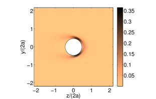
Figure 8: Contours of the mean fluid dissipation, $\langle\varepsilon\rangle$ ($v_{t}^{3}/(2a)$), averaged in the particle frame of reference.

3.3 Relative velocity

An important quantity to understand and model the settling dynamics is the particle to fluid relative motion. Although it is still unclear how to properly calculate the slip velocity between the two phases, we consider spherical shells around each particle, centered on the particles centroids, inspired by the works of Bellani & Variano (2012) and Cisse et al. (2013). We calculate the mean difference between the particle and fluid velocities in each shell as

$$\langle{\bf U}_{rel}\rangle_{{\bf x},t,NP}=\left\langle\,{\bf u}_{p}-\frac{1}{\Omega(\Delta)}\int_{\Omega(\Delta)}{\bf u}_{f}d{\cal V}\,\right\rangle_{t,NP}$$

where $\Omega(\Delta)$ is the volume of a shell of inner radius $\Delta$. A parametric study on the slip velocity is performed by changing the inner radii of these spherical shells from $\Delta=0.75$ particle diameters to $\Delta=5.0$ particle diameters, while keeping the shell thickness $\delta$ constant and equal to 0.063 in units of $2a$.

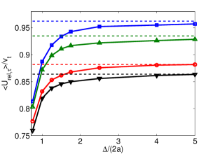
Figure 9: The component of ${\bf U}_{rel}$ aligned with gravity as a function of the shell inner radii $\Delta/(2a)$ for the four cases studied. The dashed lines represent instead the mean particles velocities in the direction of gravity, $\langle V_{p,\tau}\rangle$.

In figure 9 we report the component of ${\bf U}_{rel}$ parallel to gravity as a function of the shells inner radii $\Delta/(2a)$. As the shell inner radii increase, $|U_{rel,\tau}|$ tends exponentially to an asymptotic value which corresponds to the mean particle velocity in the same direction, $\langle V_{p,\tau}\rangle$. This is expected since the correlation between the fluid and particle velocity goes to zero at large distances. The quiescent cases still show a $0.5\%$ difference between $|U_{rel,\tau}|$ and $\langle V_{p,\tau}\rangle$ at $\Delta/(2a)=5$. This difference is again attributed to the long coherent wakes of the particles.

$\Delta/(2a)$	$\langle U_{rel,\tau}\rangle$	$\sigma_{U_{rel,\tau}}$	$S_{U_{rel,\tau}}$	$K_{U_{rel,\tau}}$
$0.75$	$+0.81$	$0.06$	$+8.040$	$123.29$
$1.00$	$+0.88$	$0.09$	$+5.655$	$68.26$
$1.25$	$+0.92$	$0.10$	$+4.547$	$47.66$
$1.50$	$+0.93$	$0.11$	$+3.912$	$37.69$
$1.75$	$+0.94$	$0.12$	$+3.482$	$31.83$
$2.50$	$+0.95$	$0.13$	$+2.919$	$24.34$
$4.00$	$+0.95$	$0.14$	$+2.18$	$16.25$
$5.00$	$+0.96$	$0.14$	$+2.22$	$17.09$

Table 5: Moments of the $pdf(U_{rel,\tau})$ for $\phi=0.5\%$ in the quiescent case. The thickness of the shell used to compute the slip velocity is $\delta/(2a)=0.063$.

$\Delta/(2a)$	$\langle U_{rel,\tau}\rangle$	$\sigma_{U_{rel,\tau}}$	$S_{U_{rel,\tau}}$	$K_{U_{rel,\tau}}$
$0.75$	$+0.76$	$0.07$	$+0.072$	$3.90$
$1.00$	$+0.83$	$0.09$	$+0.010$	$4.28$
$1.25$	$+0.85$	$0.10$	$+0.087$	$4.56$
$1.50$	$+0.86$	$0.11$	$+0.128$	$4.54$
$1.75$	$+0.87$	$0.11$	$+0.117$	$4.32$
$2.50$	$+0.87$	$0.13$	$+0.054$	$3.91$
$4.00$	$+0.88$	$0.16$	$+0.046$	$3.32$
$5.00$	$+0.88$	$0.18$	$+0.047$	$3.10$

Table 6: Moments of the $pdf(U_{rel,\tau})$ for $\phi=0.5\%$ in a turbulent environment. The thickness of the shell used to compute the slip velocity is $\delta/(2a)=0.063$.

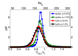
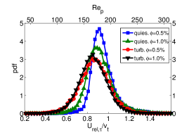
Figure 10: Comparison of the probability density functions of tangential relative velocity and corresponding particle Reynolds number $Re_{p}$. Colors and symbols are the same as previous figures. In Panel a) the cases for $\Delta/(2a)=1.5$ are reported while in panel b) we show the results for $\Delta/(2a)=2.5$.

The probability density function of these relative velocities, $U_{rel,\tau}$, and their first four central moments are computed and reported in tables 5 and 6 as a function of $\Delta/(2a)$ for the quiescent fluid and turbulent cases at $\phi=0.5\%$. In the turbulent case, the moments approach those of a Gaussian distribution with vanishing skewness and flatness close to $3$, especially at large $\Delta$. In the quiescent case, the third and fourth moments display higher values that decrease as $\Delta$ is increased, tending to the values of the particle velocities. The $pdf$s pertaining the four cases considered, calculated in spherical shells with an inner radius of $1.5$ and $2.5$ particle diameters, are compared in figure 10. A second axis, reporting the the particle Reynolds number $Re_{p}$ based on $U_{rel,\tau}$, is also displayed in each figure. In the former case, $\Delta/(2a)=1.5$, the shell radius is of the order of the Taylor scale to highlight the particle dynamics, while the relative velocity is approaching the asymptotic values for the larger shell. The $pdf$s of the relative velocity appear narrower than those of the particle absolute velocity, indicating that the particles tend to be transported by the large-scale motions, filtering the smallest scales.

The distributions pertaining the simulations in a turbulent environment are nearly Gaussian with modal values well below one. The quiescent cases show skewed distributions with long tails at high velocities, as observed for the particle velocities in figure 3a). The particles settle on average with a velocity close to that of a single particle, with occasional events of higher velocity due to the drafting-kissing-tumbling dynamics. The lower the volume fraction the more intermittent is the dynamics.

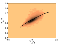
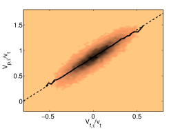
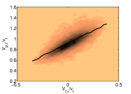
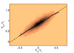
Figure 11: Joint probability distributions of $V_{f,\tau}$ and $V_{p,\tau}$ evaluated in spherical shells located at $1.75$ particle diameters from each particle. We report in panels a) and c) the quiescent cases for $\phi=0.5\%$ and $1\%$, while the respective turbulent cases are reported in panels b) and d). The continuous lines represent the integrals of the joint probability distributions. In the turbulent cases the dashed lines represent the best-fit of these integrals.

Knowing the tangential fluid velocity $\langle V_{f,\tau}\rangle_{{\bf r}}(p,t)$, averaged in each shell and at each time step, and the corresponding tangential particle velocities $V_{p,\tau}(p,t)$, it is then possible to find their joint probability distribution $P(V_{f,\tau},V_{p,\tau})$ (for sake of simplicity we write $\langle V_{f,\tau}\rangle_{{\bf r}}$ as $V_{f,\tau}$). These are evaluated in shells at $\Delta/(2a)=1.75$ for each case studied and reported in figure 11. In each case, the integral of $P(V_{f,\tau},V_{p,\tau})$,

$$\langle V_{p,\tau}|V_{f,\tau}\rangle=\int_{-\infty}^{\infty}P(V_{f,\tau},V_{p,\tau})V_{f,\tau}\,dV_{f,\tau},$$ (14)

is also reported (continuous lines). This represents the most probable particle velocity $V_{p,\tau}$ given a certain fluid velocity $V_{f,\tau}$, or, equivalently, the most probable fluid velocity surrounding a particle settling with velocity $V_{p,\tau}$. In the turbulent cases these integrals are well approximated by straight lines (displayed with dashed lines in the figure)

$$V_{p,\tau}=C_{1}V_{f,\tau}+C_{2}.$$ (15)

In both cases $C_{1}$ is approximately $1$ while $C_{2}$ is about $0.86$ for $\phi=0.5\%$ and $0.84$ for $\phi=1\%$. These values are in agreement with the values found for the average relative velocities of shells at $\Delta/(2a)=1.75$. In a quiescent flow, conversely, the integral in eq. (14) gives a curved line and no best-fit is therefore reported. In these cases, the joint probability distribution is broader, particularly in the region of higher particle velocities, $V_{p,\tau}$. This is again due to the intense particle interactions and the drafting-kissing-tumbling behaviour described in figure 4, which confirms the high flatness of the probability density functions of the relative particle velocities.

Further insight can be obtained by plotting isocontours of the average particle relative velocities and their fluctuations, in both quiescent and turbulent flows. To this end, we follow the approach by Garcia-Villalba et al. (2012). We place an uniform and structured rectangular mesh around each particle, with origin at the particle center. By means of trilinear interpolations we find the fluid and relative velocities on this local mesh and average over time and the number of particles to obtain the mean relative velocity field and its fluctuations.

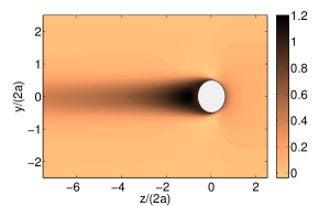
Figure 12: Contour plot of the velocity component in the direction of gravity for the single sphere settling in a quiescent fluid.

The vertical velocity of the single sphere settling in a quiescent fluid is reported in figure 12. The relative normal and tangential velocities and their fluctuations are instead displayed in figure 13 for suspensions with $\phi=0.5\%$ in both quiescent and turbulent environment. In the quiescent fluid simulations, a long wake forms behind the representative particle and, as seen from the single point particle velocity correlations, it takes a long time for this velocity fluctuations to decorrelate. In the turbulent case instead, the wakes are disrupted by the background fluctuations.

Interesting observations can be drawn from the relative velocity fluctuation fields. Comparing figures 13c) and 13d) we note that intense vortex shedding occurs around the particles in the turbulent case, with important fluctuations of $U_{rel,\tau}$. From figures 13e) and 13f) we also see that the relative velocity fluctuations are drastically increased in the horizontal directions in a turbulent environment. Noteworthy, vortex shedding occurs at particle Reynolds numbers below the critical value above which this is usually observed (Bouchet et al., 2006). Vortex shedding is unsteady in nature and unsteady effects may therefore play an important role in the increase of the overall drag, as further discussed below. Lower fluctuation intensities are found on the front part of the particles, where the energy dissipation is highest, and the immediate wake in the recirculating region where the instability is found to develop.

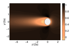
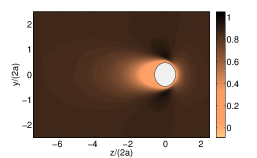
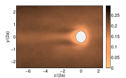
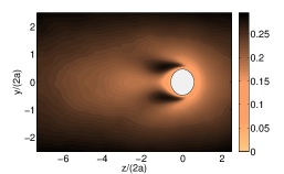
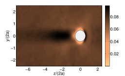
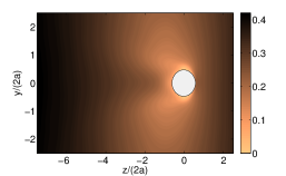
Figure 13: Fields of $\langle U_{rel,\tau}\rangle$, $U_{rel,\tau}^{\prime}$, $U_{rel,n}^{\prime}$ for the quiescent (left column) and turbulent cases (right column).

3.4 Drag analysis

As in Maxey & Riley (1983), we write the balance of the forces acting on a single sphere settling through a turbulent flow. The equation of motion for a spherical particle reads

$$\frac{4}{3}\pi a^{3}\rho_{p}\frac{d{\bf V}_{p}}{dt}=\frac{4}{3}\pi a^{3}(\rho_{p}-\rho_{f}){\bf g}+\oint_{\partial\mathcal{V}_{p}}{\bf\boldsymbol{\tau}}\cdot{\bf n}\,dS$$ (16)

where the integral is over the surface of the sphere $\partial\mathcal{V}_{p}$, ${\bf n}$ is the outward normal and ${\bf\boldsymbol{\tau}}=-p{\bf I}+2\mu{\bf E}$ is the fluid stress. As commonly done in aerodynamics, we replace the last term of equation (16) with a term depending on the relative velocity ${\bf U}_{rel}$ and a drag coefficient $C_{D}$

$$\frac{4}{3}\pi a^{3}\rho_{p}\frac{d{\bf V}_{p}}{dt}=\frac{4}{3}\pi a^{3}(\rho_{p}-\rho_{f}){\bf g}-\frac{1}{2}\rho_{f}\pi a^{2}|{\bf U}_{rel}|{\bf U}_{rel}C_{D}$$ (17)

with $\pi a^{2}$ the reference area. Generally, the drag coefficient $C_{D}$ is a function of a Reynolds number and a Strouhal number which accounts for unsteady effects. In the present case, we consider it to be a function of the Reynolds number based on the relative velocity $Re_{p}=2a|{\bf U}_{rel}|/\nu$ (in a turbulent field it is proper to define $Re_{p}$ in terms of the relative velocity between particle and fluid) and of the Strouhal number defined as

$$St=\frac{\frac{d{\bf V}_{p}}{dt}(2a)}{|{\bf U}_{rel}|^{2}}.$$ (18)

The drag on the particle depends on both nonlinear and unsteady effects (such as the Basset history force and the added mass contribution) through these two non-dimensional numbers.

Commonly, the unsteady contribution is neglected and $C_{D}$ is assumed to depend only on the Reynolds number. Since we want to investigate both nonlinear and unsteady effects, we decide to express the drag coefficient as $C_{D}(Re_{p},St)=C_{D_{0}}(Re_{p})\left[1+\psi(Re_{p},St)\right]$, yielding

$$\frac{4}{3}\pi a^{3}\rho_{p}\frac{d{\bf V}_{p}}{dt}=\frac{4}{3}\pi a^{3}(\rho_{p}-\rho_{f}){\bf g}-\frac{1}{2}\rho_{f}\pi a^{2}|{\bf U}_{rel}|{\bf U}_{rel}C_{D_{0}}(Re_{p})\left[1+\psi(Re_{p},St)\right],$$ (19)

where $\psi=0\,\forall\,Re_{p}$ if $St=0$ (steady motion). We can therefore identify a quasi-steady term and the extra term which accounts for unsteady phenomena.

By ensemble averaging equation (19) over time and the number of particles, and assuming the settling process to be at statistically steady state, we can find the most important contributions to the overall drag. The steady-state average equation reads

$$0=\frac{4}{3}\pi a^{3}(\rho_{p}-\rho_{f}){\bf g}-\frac{1}{2}\rho_{f}\pi a^{2}\left\langle|{\bf U}_{rel}|{\bf U}_{rel}C_{D_{0}}(Re_{p})\left[1+\psi(Re_{p},St)\right]\right\rangle.\\$$ (20)

Denoting the entire time dependent term simply as $\Psi(t)$ and rearranging, we obtain the following balance

$$\frac{4}{3}\pi a^{3}\left(\frac{\rho_{p}}{\rho_{f}}-1\right){\bf g}=\frac{1}{2}\pi a^{2}\langle|{\bf U}_{rel}|{\bf U}_{rel}C_{D_{0}}(Re_{p})\rangle+\Psi(t).$$ (21)

The term on the left-hand side is known whereas the time-dependent term $\Psi(t)$ is of difficult evaluation. The nonlinear steady term can be calculated using the approach described in section 3.2. At each time step we calculate the relative velocity in the spherical shells surrounding each particle. From these we compute the particle Reynolds number $Re_{p}=2a|U_{rel}|/\nu$ and using equation (8) (where we replace the terminal Reynolds number with the new particle Reynolds number) we obtain the drag coefficient. The first term on the right-hand side can therefore be evaluated by averaging over the number of particles and time steps considered. Finally we divide everything by the buoyancy acceleration to estimate the relative importance of each term

$$100\%=\mathcal{S}(Re_{p})+\Psi(t)$$ (22)

where $\mathcal{S}(Re_{p})$ represents the nonlinear steady term while the unsteady term has been denoted again as $\Psi(t)$ for simplicity.

This approach is applied to the results of the simulations of a single sphere and to the quiescent and turbulent cases with $\phi=0.5\%$ and 1%. The inner radius of the sampling shells is chosen to be $5$ particle radii and the results obtained are reported in table 7. The single sphere simulation provides an estimate of the error of the method. Since our terminal Reynolds number is smaller than the critical Reynolds number above which unsteady effects become important and our velocity field is indeed steady, the term $\Psi(t)$ should be negligible. The critical Reynolds number $Re_{c}$ has been found to be approximately $274$ by Bouchet et al. (2006) while we recall that our terminal Reynolds number for the isolated particle is $200$. The nonlinear steady term provides in this case, however, an overestimated value of the drag, with a percentage error of about $+3\%$ with respect to the buoyancy term. The possible causes of this error are the long wake and the fact that equation (8) is empirical. The data from the single-particle simulations are used to correct the results from the other runs, i.e. the data are normalized with the total drag obtained in this case. In the quiescent case at $\phi=0.5\%$, unsteady effects are negligible (about 0.5% of the total drag), while they increase to about 6% when increasing the particle evolve fraction to 1%. In a turbulent flow, importantly, we notice that the contribution of $\Psi(t)$ adds up to approximately $10\%$ of the total at $\phi=0.5\%$ and to about $12\%$ of the total at $\phi=1\%$.

Note that one can write the steady drag as mean and fluctuating component

$$\mathcal{S}(Re_{p})=\langle|{\bf U}_{rel}|{\bf U}_{rel}C_{D_{0}}(Re_{p})\rangle=\langle U_{rel}\rangle^{2}C_{D_{0}}(\langle Re_{p}\rangle)+\mathcal{S}^{\prime}(\langle Re_{p}\rangle).$$

The fluctuations $\mathcal{S}^{\prime}(\langle Re_{p}\rangle)$ would be responsible of the reduction of the settling velocity if this were to be attributed to nonlinear drag effects only (see also Wang & Maxey, 1993). We verified that for our results, the total and mean component differ by about 2%, $\langle|{\bf U}_{rel}|{\bf U}_{rel}C_{D_{0}}(Re_{p})\rangle\approx\langle U_{rel}\rangle^{2}C_{D_{0}}(\langle Re_{p}\rangle)$. This leads us to the conclusion that the main contribution to the overall drag is due to the steady term but the reduction of the mean settling velocity in a turbulent environment is almost entirely due to the various unsteady effects. These can be related to unsteady vortex shedding, see figure 13, as in the experiments of a single sphere by Mordant & Pinton (2000) These observations are also in agreements with the results in Homann et al. (2013). These authors observe that the enhancement of the drag of a sphere towed in a turbulentt environment can be explained by the modification of the mean velocity and pressure profile, and thus of the boundary layer around the sphere, by the turbulent fluctuations.

case	$\mathcal{S}(Re_{p})$	$\Psi(t)$
Quiescent $\phi=0.5\%$	$99.5\%$	$0.5\%$
Turbulent $\phi=0.5\%$	$90.4\%$	$9.6\%$
Quiescent $\phi=1.0\%$	$94.1\%$	$5.9\%$
Turbulent $\phi=1.0\%$	$87.8\%$	$12.2\%$

Table 7: Percentage contribution of the non-linear and unsteady terms for the quiescent and turbulent case with $\phi=0.5\%$. The data are normalized by the mean drag from the simulation of a single sphere in quiescent fluid.

4 Final remarks

We report numerical simulations of a suspension of rigid spherical slightly-heavy particles in a quiescent and turbulent environment using a direct-forcing immersed boundary method to capture the fluid-structure interactions. Two dilute volume fractions, $\phi=0.5\%$ and 1%, are investigated in quiescent fluid and homogeneous isotropic turbulence at $Re_{\lambda}=90$. The particle diameter is of the order of the Taylor length scale and about 12 times the dissipative Kolmogorov scale. The ratio between the sedimentation velocity and the turbulent fluctuations is about 3.4, so that the strongest fluid-particle interactions occur at approximately the Taylor scale.

The choice of the parameters is inspired by the reduction in sedimentation velocity observed experimentally in a turbulent flow by Byron (2015) and in the group of Prof. Variano at UC Berkeley. In the experiment, the isotropic homogeneous turbulence is generated in a tank of dimensions of several integral lengthscales by means of two facing randomly-actuated synthetic jet arrays (driven stochastically). The Taylor microscale Reynolds number of the experiment is $Re_{\lambda}=260$. Particle Image Velocimetry using Refractive-Index-Matched Hydrogel particles is used to measure the fluid velocity and the linear and angular velocities of finite-size particles of diameter of about $1.4$ Taylor microscales and density ratios $\rho_{p}/\rho_{f}=1.02$, $1.006$ and $1.003$. The ratio between the terminal quiescent settling velocity $v_{t}$ and the turbulence fluctuating velocity $u^{\prime}$ is about $1$, higher than in our simulations where this ratio is $3.3$. Byron (2015) observes reductions of the slip velocity between 40% and 60 % when varying the shape and density of the particles. As suggested by Byron (2015), the larger reduction in settling velocity observed in the experiments is most likely explained by the larger turbulence intensity.

The new findings reported here can be summarized as follows: i) the reduction of settling velocity in a quiescent flow due to the hindering effect is reduced at finite inertia by pair-interactions, e.g. drafting-kissing-tumbling. ii) Owing to these particle-particle interactions, sedimentation in quiescent environment presents therefore significant intermittency. iii) The particle settling velocity is further reduced in a turbulent environment due to unsteady drag effects. iv) Vortex shedding and wake disruption is served also in subcritical conditions in an already turbulent flow.

In a quiescent environment, the mean settling velocity slightly decreases from the reference value pertaining few isolated particle when the volume fraction $\phi=0.5\%$ and $\phi=1\%$. This limited reduction of the settling velocity with the volume fraction is in agreement with previous experimental findings in inertia-less and inertial flows. The Archimedes number of our particle is 21000, in the steady vertical regime before the occurrence of a first bifurcation to an asymmetric wake. In this regime, Uhlmann & Doychev (2014) observe no significant particle clustering, which is is confirmed by the present data.

The skewness and flatness of the particle velocity reveal large positive values in a quiescent fluid, and accordingly the velocity probability distribution functions display evident positive tails. This indicates a highly intermittent behavior. In particular, it is most likely to see particles sedimenting at velocity significantly higher than the mean: this is caused by the close interactions between particle pairs (more seldom triplets). Particles approaching each other draft-kiss-tumble while falling faster than the average.

In a turbulent flow, the mean sedimentation velocity further reduces, to 0.88 and 0.86 at $\phi=0.5\%$ and $\phi=1\%$. The variance of both the linear and angular velocity increases in a turbulent environment and the single-particle time correlations decay faster due to the turbulence mixing. The velocity probability distribution function are almost symmetric and tend towards a Gaussian of corresponding variance. The particle lateral dispersion is, as expected, higher in a turbulent flow, whereas the vertical one is, surprisingly, of comparable magnitude in the two regimes; this can be explained by the highly intermittent behavior observed in the quiescent fluid.

We compute the averaged relative velocity in the particle reference frame and the fluctuations around the mean. We show that the wake behind each particle is on average significantly reduced in the turbulent flow and large-amplitude unsteady motions appear on the side of the sphere in the regions of minimum pressure where vortex shedding is typically observed. The effect of a turbulent flow on the damping of the wake behind a rigid sphere has been discussed for example by Bagchi & Balachandar (2003), while the case of a spherical bubble has been investigated by Merle et al. (2005). Using the slip velocity between the particle and the fluid surrounding it, we estimate the nonlinear drag on each particle from empirical formulas and quantify the relevance of non-stationary effects on the particle sedimentation. We show that these become relevant in the turbulent regime, amount to about 10-12% of the total drag, and are responsible for the reduction of settling velocity with the respect to the quiescent flow. This can be compared with the simulations in Good et al. (2014) who attribute the reduction of the sedimentation velocity of small ($2a<\eta$) heavy ($\rho_{p}/\rho_{f}\approx 900$) spherical particles in turbulence to the nonlinear drag. Here, we show that non-stationary effects become relevant for larger particles at lower density ratios.

The present investigation can be extended in a number of interesting directions. Preliminary simulations reveal that variations of the density ratio at constant Archimedes number do not significantly modify the results presented here. It would be therefore interesting to investigate the effect of the Galileo number on the particle dynamics and of the ratio between turbulent fluctuations and sedimentation velocity.