Akari, SCUBA2 and Herschel data of pre-stellar cores

1 Introduction

Stars form in dense cores in molecular clouds. Exactly how these cores form is still a matter of debate (e.g. André at al. 2014). The cores which are gravitationally bound are known as pre-stellar cores (Ward-Thompson et al. 2007; Di Francesco et al. 2007), which then collapse to form Class 0 protostars (André et al. 1993). The mass function of cores can be modelled onto the IMF of stars (Goodwin et al. 2008). Hence cores are a significant stage in star formation. Recent work with the Akari satellite, the Herschel Space Observatory and the SCUBA2 camera on the JCMT has led to new insight into core formation (André at al. 2014).

2 Cepheus

The molecular cloud in Cepheus has been studied by many authors (e.g. Kirk et al. 2009). Figure 1 shows an extinction map of the region (Dobashi et al. 2005). North is at the top, east is to the left. The square towards the western edge of the image shows the region we have studied. This is the L1147-L1157 ring.

Figure 2 shows the extinction map (thick contours) of a close-up of the ring (Dobashi et al. 2005), superposed on a greyscale of the Digitised Sky Survey. The various molecular cloud cores from L1147 to L1157 are marked. Also shown in thin contours on Figure 2 is the Akari 90-micron emission from the region overlaid (Nutter et al. 2009). The Akari emission can be seen to be offset from the extinction peaks of both L1148 and L1155. In fact the far-infrared emission seems to be wrapping itself around the dense material (traced by extinction).

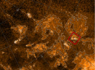
Figure 1: An extinction map of the Cepheus region (from Dobashi et al. 2005). North is at the top, east is to the left. The ring of cores being studied here is indicated by a box towards the western edge of this image.

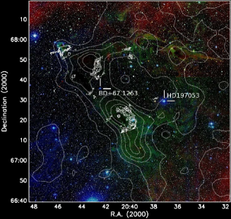
Figure 2: A close-up of the extinction map (thick contours) of the Cepheus cloud showing the region in the box indicated in Figure 1 (from Dobashi et al. 2005). This is the L1147-L1157 region. The underlying image is from the Digitized Sky Survey. The Akari 90-micron emission is superposed as thin contours (Nutter et al. 2009).

We therefore hypothesise that the 90-micron emission is tracing slightly warmer dust around the edges of these cores. This is what would be predicted if the cores were being externally heated. Two potential heating sources were located. However, due to the geometry and nature of the stars involved, we deduced that the core heating was due to the star HD197053 (Nutter et al. 2009).

3 Ophiuchus

Figure 3 shows the Ophiuchus molecular cloud as seen by Herschel at 70 to 250 microns (Pattle et al. 2015). North is at the top, east is to the left. The Oph A core can be seen clearly at the top centre of the image, with the other cores to the south-east. Combining these data with Herschel data allows us to calculate the temperature of the emitting dust, and hence its mass. We can then calculate the total mass of each core using canonical gas-to-dust mass ratios. Other studies have looked at the dense gas in Ophiuchus using different tracers. For example, André et al. (2007) studied $N2H+$ in the region. We have used their data to calculate a virial mass for each of our cores.

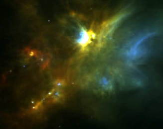
Figure 3: Composite 70/160/250 image of the Ophiuchus L1688 cloud (Ladjelate et al. 2014; Pattle et al. 2015). Oph A is the bright region in the upper centre of the image.

Figure 4: Plot of virial mass derived from $N2H+$ against core mass derived from the dust emission, as measured from SCUBA2 and Herschel data (Pattle et al. 2015).

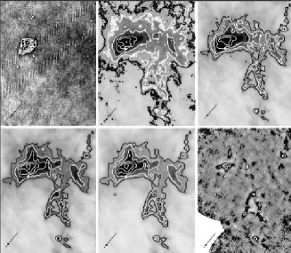
Figure 5: Herschel and SCUBA2 images of the L1495 molecular cloud in Taurus. Top row, left to right: 60, 170 and 250 microns respectively. Lower row, left to right: 350, 500 and 850 (from SCUBA2) microns respectively. Note how SCUBA2 only detects some of the cores seen at the other wavelengths by Herschel (Ward-Thompson et al. 2014).

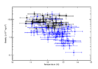
Figure 6: Plot of density versus temperature for the starless cores in L1495. Those detected by SCUBA2 (in black) all lie to the upper left-hand side of the plot (Ward-Thompson et al. 2014), indicating that SCUBA2 is only sensitive to the coldest, densest cores.

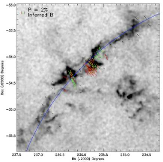
Figure 7: Greyscale Herschel image of part of the Lupus I molecular cloud. Magnetic field vectors deduced from BLAST polarisation mapping are overlaid. The filament is traced with a curved solid line. Note how the magnetic field lies mostly perpendicular to the direction of the filament (Matthews et al. 2014).

Figure 8: Model of star formation consistent with the data (from André at al. 2014). Matter flows first along magnetic field lines onto filaments. Parts of each filament become ‘seed’ cores. Matter then flows along the filament onto the cores. When the mass per unit length of thefilament exceeds the critical value the cores collapse (from André at al. 2014).

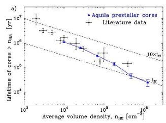
Figure 9: Plot of mean lifetime versus mean column density for a sample of cores from the literature (Jessop & Ward-Thompson 2000) and from Herschel data on the Aquila region (Könyves et al. 2014). The best fit to the data is steepr than predicted by free-fall collapse (from André at al. 2014).

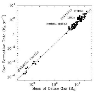
Figure 10: Plot showing the relation between star formation rate and mass of dense gas (after Lada et al. 2012). The dashed line is found by inverting the best-fit line from Figure 9 (see Könyves et al. 2014). The line is seen to be consistent with the data, and may provide an explanation for the Schmidt-Kennicutt Law (from André at al. 2014).

Figure 4 shows a plot of core virial mass against observed mass derived from SCUBA2 and Herschel data (Pattle et al. 2015). By looking at where each individual core lies on this plot, we are able to plot a trend in the data from upper right to lower left in this plot, which correlates with a trend in location from north-west to south-east in Figure 3.

We can explain this in terms of the degree of gravitational boundedness of the cores. Those to the western side of Figure 3 are more tightly gravitationally bound than those to east. We interpret this in terms of sequential star formation from west to east in this image (Pattle et al. 2015).

The more tightly gravitationally bound cores to the west are interpreted as being more evolved than those towards the east. This is consistent with a previously proposed hypothesis for the star formation in Ophiuchus, comparing L1688 to L1689 (Nutter et al. 2006).

These latter authors found that star formation in L1688 had progressed much further than in L1689, referring to L1689 as the ‘dog that didn’t bark’. This was interpreted as being caused by the external influence of the Upper Sco OB association to the west of Ophiuchus triggering star formation in L1688 before L1689. This trend is exactly consistent with what we see in the SCUBA2 and Herschel data (Pattle et al. 2015).

Therefore, in both Cepheus and Ophiuchus we see the evolution of cores being heavily influenced by their surroundings and their environment. In particular, in Ophiuchus we are seeing an apparent case of sequential star formation from west to east across the region.

4 Taurus

Figure 5 shows the L1495 region in Taurus (Ward-Thompson et al. 2014). Five Herschel wavebands and one waveband from SCUBA2 are shown. A number of cores and filamentary structures can be seen. In particular a triangle-shaped arrangement of filaments can be seen just below centre of each image. The ubiquity of filaments is a feature seen in almost all of the Herschel data of star-forming regions (André at al. 2014).

The bright region towards the upper part of the image that is seen at most wavebands is the L1495A core, and is exactly coincident with L1495A-S. This lies at the head of a large, filamentary structure that is seen clearly in the Herschel data of the Taurus region (Marsh et al. 2014). We measured a temperature gradient across this core, with the hotter material lying to the south (Ward-Thompson et al. 2014).

There is a bright star, slightly to the south of L1495A-S, which is known as V892 Tau (IRAS04155+2812). This is a Herbig Ae/Be star, and it is clearly heating L1495A-S, which is otherwise starless, and causing the temperature gradient across the core. This is very similar to that seen in the Cepheus discussed above. So once again we see that environment is affecting evolution.

Note that only some of the cores visible in the Herschel images are seen in the SCUBA2 image. These regions are seen most clearly by SCUBA2 at 850 $\mu$m, but not seen so clearly at shorter wavelengths by Herschel. Note, for example the filament to the upper right in the Herschel images, which appears to Herschel as no different from the other filaments, but which is almost invisible in the SCUBA2 images.

Figure 6 shows a plot of density versus temperature for the cores in L1495. The cores not detected by SCUBA2 are indicated by a different symbol from those thare detected by SCUBA2. Note that the cores not detected by SCUBA2 all lie to the lower right-hand side of this plot (Ward-Thompson et al. 2014). This indicates that SCUBA2 is only sensitive to the coldest, densest cores, whereas Herschel sees all of the cores.

5 Lupus

Figure 7 shows a Herschel image of the Lupus I molecular cloud. Magnetic field vectors deduced from BLAST polarisation mapping are overlaid (Matthews et al. 2014). The filament is traced with a curved solid line. Note how the magnetic field lies mostly perpendicular to the direction of the filament (Matthews et al. 2014).

This is consistent with other observations of filaments and magnetic fields (palmerim2013). This has led to a model being proposed for star formation that invokes the magnetic field funnelling material onto filaments (André at al. 2014). Material then flows along filaments to form cores (Balsara et al. 2001; André at al. 2014). When sufficient mass has accreted in a core that the filament’s critical mass-to-flux ratio is exceeded the core collapses (Inutsuka & Miyama 1997).

The observation that the majority of cores form on filaments (Könyves et al. 2010) indicates that this is the dominant mode of star formation. Observation of flows along filaments has been observed before (e.g. Balsara et al. 2001), but the new observations give the first indication of flow onto filaments (Palmeirim et al. 2013).

6 Discussion

Figure 9 shows a plot of lifetime versus mean density for samples of dense cores that was originally proposed by Jessop & Ward-Thompson (2000). A general trend was observed that was steeper than that predicted by free-fall collapse. More recent Herschel data also show this same trend (Könyves et al. 2014).

André et al. (2014) have proposed that this trend may in fact explain the Schmidt-Kennicutt Law, in its recent incarnation by Lada et al. (2012). If the best-fit line from Figure 9 is converted into a star formation rate and account is taken of the filamentary nature of the clouds of dense gas above the star-forming threshold (Lada et al. 2012), then for Aquila we derived a star formation rate, given by $SFR=4.5\times 10^{-8}M_{\odot}yr^{-1}\times(M_{\rm dense}/M_{\odot})$ (Könyves et al. 2014).

Figure 10 shows a plot of star formation rate against mass of dense gas above the star-forming threshold (after Lada et al. 2012), showing both Galactic clouds and external galaxies from normal spirals to ULIRGs (Gao & Soloman 2004). Also shown on this plot as a dashed line is the star formation mentioned above, as derived from Herschel data of Aquila (Könyves et al. 2014) and earlier data (Jessop & Ward-Thompson 2000).

The dashed line fits exactly to the data of both our own Galaxy and of external galaxies. This led us to hypothesise that the filamentary nature of molecular clouds, and the core life-time versus density relation, may ultimately lead to a universal law for star formation (André at al. 2014).

7 Conclusions

We have shown data from Akari, Herschel and SCUBA-2 of pre-stellar cores in the star-forming regions in Cepheus, Ophiuchus, Taurus and Lupus. A number of themes have emerged:

• We have seen that the environment in which the cores exist is extremely important. For example, in Cepheus and Ophiuchus the external effects of nearby luminous stars is causing temperature gradients across the clouds. In the case of Ophiuchus we are also seeing sequential star formation.

• In Taurus we have compared and contrasted the Herschel data with the SCUBA2 data and seen that whereas Herschel is seen to be sensitive to all structures, SCUBA2 only picks up the coldest, densest cores that are probably pre-stellar in nature.

• In Taurus and Lupus we have seen examples of filamentary molecular clouds that are seen to be everywhere in the Taurus data. In fact, the Herschel data show that core formation on filaments is the dominant mode of star formation (André et al. 2010).

• We have seen how the magnetic field in Lupus lies perpendicular to the main filament, supporting a model of star formation in which the magnetic field funnels material onto filaments, and material flows along the filaments onto cores (André at al. 2014).

• We have seen how observations of the life-time versus density relation, together with Herschel observations of Aquila, lead to a new explanation of the star-formation versus dense gas mass relation (André at al. 2014).

It is clear that these far-infrared and submm instruments have changed our views about star formation.

References

- André et al. (1993) André et al., 1993, ApJ 406, 122
- André et al. (2007) André et al., 2007, A&A 472, 519
- André et al. (2010) André et al., 2010, A&A 518, L102
- André at al. (2014) André et al., 2014, arXiv:1312.6232
- Balsara et al. (2001) Balsara et al., 2001, MNRAS 327, 715
- Di Francesco et al. (2007) Di Francesco et al., 2007, PPV, 17
- Dobashi et al. (2005) Dobashi et al., 2005, PASJ 57, 1
- Gao & Soloman (2004) Gao & Solomon, 2004, ApJ 606, 271
- Goodwin et al. (2008) Goodwin et al., 2008, A&A 477, 823
- Inutsuka & Miyama (1997) Inutsuka & Miyama, 1997, ApJ 480, 681
- Jessop & Ward-Thompson (2000) Jessop & Ward-Thompson, 2000, MNRAS 311, 63
- Kirk et al. (2009) Kirk et al., 2009, ApJS 185, 198
- Könyves et al. (2010) Könyves et al., 2010, A&A 518, L106
- Könyves et al. (2014) Könyves et al., 2014, in prep.
- Lada et al. (2012) Lada et al., 2012, ApJ 745, 190
- Ladjelate et al. (2014) Ladjelate et al., 2014, in prep.
- Marsh et al. (2014) Marsh et al., 2014, in prep.
- Matthews et al. (2014) Matthews et al., 2014, ApJ 784, 116
- Nutter et al. (2006) Nutter et al., 2006, MNRAS 368, 1833
- Nutter et al. (2009) Nutter et al., 2009, MNRAS 396, 1851
- Palmeirim et al. (2013) Palmeirim et al., 2013, A&A 550, A38
- Pattle et al. (2015) Pattle et al., 2015, arXiv:1502.05858
- Ward-Thompson et al. (2007) Ward-Thompson et al., 2007, PPV, 33
- Ward-Thompson et al. (2014) Ward-Thompson et al., 2014, in prep.