Remarks on Legendrian Self-Linking

Abstract

The Thurston-Bennequin invariant provides one notion of self-linking for any homologically-trivial Legendrian curve in a contact three-manifold. Here we discuss related analytic notions of self-linking for Legendrian knots in ${\mathbb{R}}^{3}$. Our definition is based upon a reformulation of the elementary Gauss linking integral and is motivated by ideas from supersymmetric gauge theory. We recover the Thurston-Bennequin invariant as a special case.

I Introduction

The linking number $\operatorname{\mathsf{lk}}(C_{1},C_{2})$ of disjoint, oriented curves ${C_{1},C_{2}\subset{\mathbb{R}}^{3}}$ is among the most basic invariants in knot theory, and as such it admits many different descriptions. We begin with three.

Let $(x,y,z)$ be Euclidean coordinates on ${\mathbb{R}}^{3}$ and consider the global angular form BottTu:82

$$\psi\,=\,\frac{1}{4\pi}\frac{x\,dy{\wedge}dz\,-\,y\,dx{\wedge}dz\,+\,z\,dx{\wedge}dy}{\left[x^{2}\,+\,y^{2}\,+\,z^{2}\right]^{3/2}}\,\in\,\Omega^{2}\big{(}{\mathbb{R}}^{3}-\{0\}\big{)}\,.$$ (1)

With the given normalization, ${\psi=\varrho^{*}\omega}$ is the pullback of an $SO(3)$-invariant, unit-volume form $\omega$ on ${S^{2}\subset{\mathbb{R}}^{3}}$ under the retraction

$$\varrho:{\mathbb{R}}^{3}-\{0\}\,\longrightarrow\,S^{2}\,,$$ (2)

$$\varrho(x,y,z)\,=\,\frac{\left(x,y,z\right)}{\left[x^{2}\,+\,y^{2}\,+\,z^{2}\right]^{1/2}}\,.$$

Without loss, we take the embedded curves ${C_{i}}$ for ${i=1,2}$ to be parametrized by smooth maps

$$X_{i}:S^{1}\,\longrightarrow\,{\mathbb{R}}^{3}\,,\qquad i=1,2\,,$$ (3)

in terms of which we write the difference

$$\Gamma:{\mathbb{R}}^{3}\times{\mathbb{R}}^{3}\,\longrightarrow\,{\mathbb{R}}^{3}\,,$$ (4)

$$\Gamma(X_{1},X_{2})\,=\,X_{2}-X_{1}\,.$$

The Gauss formula for the linking number of $C_{1}$ and $C_{2}$ is then given by an integral over the torus ${T^{2}=S^{1}\times S^{1}}$,

$$\operatorname{\mathsf{lk}}(C_{1},C_{2})\,=\,\int_{T^{2}}\left(X_{1}\times X_{2}\right)^{*}\!\Gamma^{*}\psi\,.$$ (5)

Essential here, since $C_{1}$ and $C_{2}$ are disjoint space curves, the singularity of $\psi$ at the origin is avoided, and the Gauss integrand is everywhere smooth and bounded on $T^{2}$.

Alternatively, because $\omega$ represents a generator for the cohomology $H^{2}(S^{2};{\mathbb{Z}})$, the Gauss linking integral computes the topological degree

$$\operatorname{\mathsf{lk}}(C_{1},C_{2})\,=\,\deg\varphi_{12}\,\in\,{\mathbb{Z}}\,,$$ (6)

where $\varphi_{12}$ is the composition

$$\varphi_{12}:T^{2}\,\longrightarrow\,S^{2}\,,\qquad\qquad\varphi_{12}\,=\,\varrho\circ\Gamma\circ(X_{1}\times X_{2})\,.$$ (7)

In its second description as the degree of $\varphi_{12}$, the linking number is clearly an integer and invariant under smooth isotopies of the curves $C_{1,2}$. The overall sign of the linking number depends upon the orientations for $T^{2}$ and $S^{2}$. Throughout, if $(\theta_{1},\theta_{2})$ are angular coordinates on $T^{2}$, we orient the torus by $d\theta_{1}{\wedge}d\theta_{2}$. We similarly give ${S^{2}\subset{\mathbb{R}}^{3}}$ the orientation induced from the standard orientation $dx{\wedge}dy{\wedge}dz$, for which the cohomology generator ${\omega>0}$ is positive.

$$\begin{matrix}&\includegraphics[scale={0.50}]{over.eps}\qquad&\qquad&\includegraphics[scale={0.50}]{under.eps}\\ &(a.)\quad\operatorname{\mathsf{w}}=+1\qquad&\qquad&(b.)\quad\operatorname{\mathsf{w}}=-1\end{matrix}$$

Figure 1: Writhe at right- and left-handed crossings.

Famously the linking number admits a third, diagrammatic description, convenient for computations. Again without loss, we consider a generic plane projection for $C_{1}$ and $C_{2}$ in which only simple, double-point crossings are present. The index set I of all crossings in the planar diagram for the link divides into subsets ${\textbf{I}=\textbf{I}^{1}_{1}\cup\textbf{I}^{1}_{2}\cup\textbf{I}^{2}_{1}\cup\textbf{I}^{2}_{2}}$, depending upon whether the upper and lower strands at each crossing belong respectively to $C_{1}$ or $C_{2}$. To each crossing ${a\in\textbf{I}}$ we attach a local writhe ${\operatorname{\mathsf{w}}_{a}=\pm 1}$ according to the handedness, as in Figure 1. In terms of these data, the linking number is computed by any of the following sums,

$$\operatorname{\mathsf{lk}}(C_{1},C_{2})\,=\,\sum_{a\in\textbf{I}^{2}_{1}}\operatorname{\mathsf{w}}_{a}\,=\,\sum_{b\in\textbf{I}^{1}_{2}}\operatorname{\mathsf{w}}_{b}\,=\,\frac{1}{2}\sum_{c\in\textbf{I}^{2}_{1}\cup\textbf{I}^{1}_{2}}\operatorname{\mathsf{w}}_{c}\,.$$ (8)

The signed sum of crossings by $C_{2}$ over $C_{1}$ can be interpreted as a signed count of preimages $\varphi_{12}^{-1}(p)$ for ${p\in S^{2}}$ at the North Pole, so the first equality in (8) follows directly from the topological description of $\operatorname{\mathsf{lk}}(C_{1},C_{2})$ as the degree of $\varphi_{12}$. One can check that our orientation conventions for $T^{2}$ and $S^{2}$ are consistent with the assignment of signs for $\operatorname{\mathsf{w}}$ in Figure 1. The second equality in (8) follows similarly with ${p\in S^{2}}$ at the South Pole, and the third equality is the symmetric combination of the preceding two.

I.1 Perspectives on self-linking

The present article is concerned not with linking but with self-linking, for which one would like to make sense of $\operatorname{\mathsf{lk}}(C_{1},C_{2})$ as a knot invariant in the degenerate case ${C_{1}=C_{2}}$. This problem does not have a unique solution, and several notions of self-linking already exist. Our purpose is to propose another, motivated by gauge theory Beasley:2015 ; ZhangR:2016 and with an eye towards higher-order self-linking invariants, defined in the geometric style of Bott:95g as integrals over configuration spaces of points associated to the knot.

The most naive attempt to define a self-linking number for an embedded, oriented curve ${C\subset{\mathbb{R}}^{3}}$ is based upon the Gauss integral in (5). Again parametrizing $C$ as the image of a smooth map

$$X:S^{1}\,\longrightarrow\,{\mathbb{R}}^{3}\,,$$ (9)

we follow our nose to set

$$\operatorname{\mathsf{slk}}_{0}(C)\,:=\,\underset{\varepsilon\to 0}{\lim}\int_{T^{2}-\Delta(\varepsilon)}\left(X\times X\right)^{*}\!\Gamma^{*}\psi\,.$$ (10)

Unlike (5), the self-linking integrand is now singular along the diagonal ${\Delta\subset T^{2}}$, due to the divergence of $\psi$ at the origin in ${\mathbb{R}}^{3}$. To deal with the singularity, we excise a tubular neighborhood $\Delta(\varepsilon)$ of width ${0<\varepsilon\ll 1}$ about the diagonal, depicted as the shaded region in Figure 2, and we integrate only over the resulting cylinder ${T^{2}-\Delta(\varepsilon)}$. We finally take the limit ${\varepsilon\to 0}$ to remove any dependence on the auxiliary parameter.

$$\begin{matrix}\raisebox{-60.0pt}{\includegraphics[scale={0.60}]{Deleps.eps}}\,&\simeq\,\,\,\raisebox{-42.0pt}{\includegraphics[scale={0.30}]{Cyl.eps}}\end{matrix}$$

Figure 2: Neighborhood $\Delta(\varepsilon)$ of the diagonal in ${T^{2}}$.

There are two essential statements to make about the naive self-linking integral in (10), both of which go back to the classic works by Călugăreanu Calugareanu:59 and Pohl Pohl:67 . First, the singularity along the diagonal $\Delta$ is integrable, so the limit defining ${\operatorname{\mathsf{slk}}_{0}(C)\in{\mathbb{R}}}$ does exist.

Second, $\operatorname{\mathsf{slk}}_{0}(C)$ is not a deformation-invariant of $C$, but rather varies to first-order under a change $\delta X$ in the embedding,

$$\delta\operatorname{\mathsf{slk}}_{0}(C)\,=\,-\frac{1}{2\pi}\oint_{S^{1}}\!\!ds\,\,\epsilon_{\mu\nu\rho}\,\dot{X}^{\mu}\,\delta X^{\nu}\,\raisebox{1.25pt}{$\dddot{X}{}^{\!\rho}$}\,,\qquad\qquad||\dot{X}(s)||^{2}\,=\,1\,.$$ (11)

To simplify the expression on the right of (11), we have taken $X^{\mu}(s)$ to be a regular, unit-speed parametrization, ${\dot{X}^{\mu}\equiv dX^{\mu}/ds}$, for which $ds$ is the arc-length measure on $C$. Also, $\epsilon_{\mu\nu\rho}$ for ${\mu,\nu,\rho=1,2,3}$ is the fully anti-symmetric tensor, normalized so that ${\epsilon_{123}=+1}$. As a corollary of (11), the value of the naive self-linking integral depends non-trivially on the geometry of ${C\subset{\mathbb{R}}^{3}}$, and it cannot generically be an integer, ${\operatorname{\mathsf{slk}}_{0}(C)\notin{\mathbb{Z}}}$.

The naive attempt to define a self-linking invariant fails for two reasons, one topological and one analytic.

From the topological perspective, the primary difficulty is that the domain of integration ${T^{2}-\Delta(\varepsilon)}$ has a boundary, illustrated in Figure 2. When the embedding map $X$ varies in (10), the integrand changes by a cohomologically-trivial two-form, whose integral over the cylinder ${T^{2}-\Delta(\varepsilon)}$ receives a non-trivial boundary contribution for ${\varepsilon>0}$.

The analytic aspect of the self-linking anomaly is not as obvious, but no less important. To wit, in the detailed computation leading to (11), the boundary contribution to $\delta\operatorname{\mathsf{slk}}_{0}(C)$ remains non-vanishing even in the limit ${\varepsilon\to 0}$. See the Ph.D. thesis of Bar-Natan BarNatan:91 for a very nice presentation of the anomaly calculation. This phenomenon depends very much on the analytic behavior of the angular form $\psi$ near the origin, and need not have occurred had the divergence of $\psi$ been less rapid. This observation will be central to our work and is exemplified by the Fundamental Lemma in Section II.

Because of the anomaly, all notions of self-linking involve a modification to the naive Gauss integral in (10), as well as a refinement of the equivalence relation by smooth isotopy for the curve ${C\subset{\mathbb{R}}^{3}}$.

For instance, in the original approach of Calugareanu:59 ; Pohl:67 , one adds to $\operatorname{\mathsf{slk}}_{0}(C)$ a counterterm $T(C)$ whose variation with respect to $X$ is exactly opposite the variation in (11),

$$\delta T(C)\,=\,-\delta\operatorname{\mathsf{slk}}_{0}(C)\,.$$ (12)

The required counterterm is nothing more than the total torsion of $C$ measured with respect to arc-length,

$$T(C)\,=\,\frac{1}{2\pi}\oint_{S^{1}}\!\!ds\,\,\tau\,,$$ (13)

where the local Frenet-Serret doCarmo:76 torsion $\tau$ is given in terms of $X$ by

$$\tau\,=\,\frac{\epsilon_{\mu\nu\rho}\,\dot{X}^{\mu}\,\ddot{X}^{\nu}\,\raisebox{1.25pt}{$\dddot{X}{}^{\!\rho}$}}{||\dot{X}\times\ddot{X}||^{2}}\,,\qquad\qquad\ddot{X}(s)\,\neq\,0\,.$$ (14)

For sake of brevity, we do not review the proof of (12) here. A direct calculation of $\delta T(C)$ can be found in Appendix B of Beasley:2015 .

From the relation in (12), the sum

$$\operatorname{\mathsf{slk}}_{\tau}(C)\,=\,\operatorname{\mathsf{slk}}_{0}(C)\,+\,T(C)\,$$ (15)

does not change under any small deformation of $C$, so it provides a reasonable notion of self-linking. However, $\operatorname{\mathsf{slk}}_{\tau}(C)$ is also not invariant under arbitrary smooth isotopies of $C$. Due to the denominator in (14), the torsion $\tau$ is only defined at points of $C$ where ${\ddot{X}(s)\neq 0}$, or equivalently, where the Frenet-Serret curvature is non-zero. To make sense of $T(C)$, we assume that $C$ has everywhere non-vanishing curvature. The latter condition is open and so holds for the generic space curve, but of course it does not hold for all space curves. As a result, $\operatorname{\mathsf{slk}}_{\tau}(C)$ is only invariant under those ‘non-degenerate’ isotopies which preserve the condition of non-vanishing curvature along $C$.

Figure 3: Trefoil knot with ${\operatorname{\mathsf{w}}(C)=-3}$.

Like the linking number, the self-linking number in (15) has a simple diagrammatic description. To derive it, consider the smooth isotopy

$$F_{\Lambda}:{\mathbb{R}}^{3}\,\longrightarrow\,{\mathbb{R}}^{3}\,,\qquad\qquad F_{\Lambda}(x,y,z)\,=\,\left(x,y,\frac{z}{\Lambda}\right),$$ (16)

where ${\Lambda>0}$ is a positive real parameter. Applied to any curve ${C\subset{\mathbb{R}}^{3}}$, this isotopy flattens $C$ to the $xy$-plane as $\Lambda$ grows to infinity. Rotating $C$ if necessary, we assume that both $C$ and its projection to the $xy$-plane have everywhere non-vanishing curvature. See Figure 3 for a diagram of the trefoil knot which satisfies this condition. Then $F_{\Lambda}$ is non-degenerate for all values of $\Lambda$, and $\operatorname{\mathsf{slk}}_{\tau}(C)$ can be evaluated in the limit ${\Lambda\to\infty}$. For any plane curve, ${\tau=0}$ identically, so $\operatorname{\mathsf{slk}}_{\tau}(C)$ reduces to $\operatorname{\mathsf{slk}}_{0}(C)$ in this limit. Otherwise, when $\Lambda$ is large and $C$ is nearly planar, the naive self-linking integral in (10) reduces to a sum over the local writhe at each self-crossing of $C$. We omit a proof of the latter claim, which is hopefully plausible on the basis of the similar description (8) for $\operatorname{\mathsf{lk}}(C_{1},C_{2})$. In Section III.1, we will establish a closely related result as part of our Main Theorem.

Altogether, $\operatorname{\mathsf{slk}}_{\tau}(C)$ is given by the writhe $\operatorname{\mathsf{w}}(C)$ of the planar diagram for $C$,

$$\operatorname{\mathsf{slk}}_{\tau}(C)\,=\,\operatorname{\mathsf{w}}(C)\,:=\,\sum_{a\in\textbf{I}}\operatorname{\mathsf{w}}_{a}\,.$$ (17)

In particular, ${\operatorname{\mathsf{slk}}_{\tau}(C)\in{\mathbb{Z}}}$ is an integer, which is not manifest from the analytic description. Also, because the assignment of the writhe ${\operatorname{\mathsf{w}}=\pm 1}$ in Figure 1 is invariant under a reversal of orientation for both strands, $\operatorname{\mathsf{slk}}_{\tau}(C)$ does not depend upon the orientation of $C$. Finally, the various versions of the unknot in Figure 4 illustrate that $\operatorname{\mathsf{slk}}_{\tau}(C)$ cannot be a full isotopy invariant of $C$.

$$\begin{matrix}&\includegraphics[scale={0.50}]{unknot1.eps}\qquad&\qquad\includegraphics[scale={0.50}]{unknot2.eps}\qquad&\qquad\includegraphics[scale={0.50}]{unknot3.eps}\\[4.30554pt] &(a.)\quad\operatorname{\mathsf{w}}(C)=0\qquad&\qquad(b.)\quad\operatorname{\mathsf{w}}(C)=1\qquad&\qquad(c.)\quad\operatorname{\mathsf{w}}(C)=2\end{matrix}$$

Figure 4: Writhe for a selection of unknots.

The Frenet-Serret self-linking number $\operatorname{\mathsf{slk}}_{\tau}(C)$ is really a special case of the more general, and perhaps more familiar, notion of framed self-linking. By definition, a framing of ${C\subset{\mathbb{R}}^{3}}$ is a trivialization of the normal bundle $N_{C}$, up to homotopy. Such a trivialization can be specified by a nowhere-vanishing normal vector field ${n\in\Gamma(C,N_{C})}$ along the knot. In turn, the normal vector field determines a new curve $C_{n}$ obtained by displacing $C$ a small amount in the direction of $n$, as shown in Figure 5.

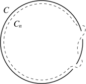
Figure 5: A framed unknot, with ${\operatorname{\mathsf{slk}}_{\rm f}(C,n)=2}$.

Given the pair $(C,n)$, the framed self-linking number is defined as the ordinary linking number of the two disjoint curves $C$ and $C_{n}$,

$$\operatorname{\mathsf{slk}}_{\rm f}(C,n)\,:=\,\operatorname{\mathsf{lk}}(C,C_{n})\,.$$ (18)

On the upside, $\operatorname{\mathsf{slk}}_{\rm f}(C,n)$ is manifestly an integral isotopy invariant of the pair $(C,n)$. On the downside, $\operatorname{\mathsf{slk}}_{\rm f}(C,n)$ carries no information about the knot $C$ itself, since the invariant takes all possible values as the winding number of $n$ about $C$ shifts.

Had one a canonical choice of framing, the framed self-linking number $\operatorname{\mathsf{slk}}_{\rm f}(C,n)$ could be converted into an honest invariant of $C$. No such choice exists for all smooth curves simultaneously, but a variety of choices can be made if one restricts to special classes of curves.

We have already encountered an example in the discussion of the Frenet-Serret self-linking $\operatorname{\mathsf{slk}}_{\tau}(C)$, for which we require ${C\subset{\mathbb{R}}^{3}}$ to have everywhere non-vanishing curvature. Not coincidentally, such curves also carry a canonical Frenet-Serret framing, with unit normal ${n=\ddot{X}/||\ddot{X}||}$. Indeed, a natural guess is that ${\operatorname{\mathsf{slk}}_{\tau}(C)=\operatorname{\mathsf{slk}}_{\rm f}(C,n)}$ for the Frenet-Serret normal.

This guess is correct, as can be seen most easily by considering the behavior of the Frenet-Serret frame in the planar limit ${\Lambda\to\infty}$ from (16). In this limit, the Frenet-Serret framing reduces to the blackboard framing in which the unit normal vector $n$ lies everywhere in the plane of the knot diagram. After displacing $C$ by $n$, one finds a planar ribbon graph, shown in the neighborhood of a positive crossing on the left in Figure 6. For such a graph, each self-crossing of $C$ corresponds to a crossing of $C$ by $C_{n}$ with identical chirality, so automatically ${\operatorname{\mathsf{w}}(C)=\operatorname{\mathsf{lk}}(C,C_{n})}$. The relation between the writhe and the Frenet-Serret framing can also be understood in three-dimensional terms, as indicated to the right in Figure 6.

$$\begin{matrix}&\raisebox{-23.0pt}{\includegraphics[scale={0.50}]{ribbon.eps}}\quad&\simeq\quad&\raisebox{-40.0pt}{\includegraphics[scale={0.50}]{twist.eps}}\\[6.45831pt] &\operatorname{\mathsf{w}}\,=\,+1\qquad&\qquad&\operatorname{\mathsf{slk}}_{\rm f}\,=\,+1\end{matrix}$$

Figure 6: Relation between writhe and Frenet-Serret framing.

I.2 Legendrian knots

This article serves as the companion to a longer work Beasley:2015 in which we develop a new, effectively supersymmetric formulation of Chern-Simons perturbation theory. Both the Frenet-Serret and the framed self-linking invariants were rediscovered physically Guadagnini:91g ; Polyakov:1988md ; Witten:1989hf in the setting of bosonic Chern-Simons theory, and our purpose is to present what one finds with the addition of ${{\mathcal{N}}=2}$ supersymmetry, after all the baggage from gauge theory is removed. Details about the gauge theory are discussed in Beasley:2015 ; ZhangR:2016 .

Supersymmetry has two consequences. We discuss the first now, and we defer a discussion of the second to the next subsection.

As a first consequence of supersymmetry, ${C\subset{\mathbb{R}}^{3}}$ must be Legendrian with respect to the standard contact structure on ${\mathbb{R}}^{3}$, and the supersymmetric self-linking number will be a Legendrian isotopy invariant. For very enjoyable introductions to contact topology and the study of Legendrian knots, see Etnyre:2003 ; Etnyre:2006j ; Geiges:2006 ; Geiges:2008 . At the moment, we recall only the minimum necessary to state and prove our Main Theorem.

Throughout, we represent the standard contact structure on ${\mathbb{R}}^{3}$ with the contact form

$$\kappa\,=\,dz\,+\,x\,dy\,-\,y\,dx\,,$$ (19)

for which the top-form ${\kappa{\wedge}d\kappa>0}$ is positive with respect to the standard orientation on ${\mathbb{R}}^{3}$. This choice of contact form respects many symmetries, which are important here and in Beasley:2015 ; ZhangR:2016 .

Manifestly, $\kappa$ is preserved under translations generated by the Reeb field ${{\mathsf{R}}=\partial/\partial z}$ as well as rotations in the $xy$-plane. Though $\kappa$ is not preserved by translations in the $xy$-plane, $\kappa$ is preserved by the left-action of the Heisenberg Lie group ${{\mathbb{H}}\simeq{\mathbb{R}}^{3}}$ on itself, where the Heisenberg multiplication ${\mu:{\mathbb{H}}\times{\mathbb{H}}\to{\mathbb{H}}}$ is given by

$$\mu\big{(}X_{1},X_{2}\big{)}\,=\,\left(x_{1}+x_{2},\,y_{1}+y_{2},\,z_{1}+z_{2}-x_{1}y_{2}+x_{2}y_{1}\right),\qquad X_{1,2}\,\in\,{\mathbb{H}}\,.$$ (20)

The origin remains the identity in ${\mathbb{H}}$, and the Heisenberg inverse is ${X^{-1}=\left(-x,-y,-z\right)}$. Finally, $\kappa$ is homogeneous of degree two under the parabolic scaling

$$(x,y,z)\,\longmapsto\,\left(\lambda x,\,\lambda y,\,\lambda^{2}z\right),\qquad\qquad\lambda\,\in\,{\mathbb{R}}_{+}\,,$$ (21)

which commutes with Heisenberg multiplication. As a result, the parabolic scaling fixes each contact plane ${H\subset{\mathbb{R}}^{3}}$ in the kernel of $\kappa$.

A picture of the family of contact planes ${H=\ker\kappa}$ appears in Figure 7. The contact planes are approximately horizontal near ${x=y=0}$, but they twist vertically as one moves outward from the origin in the $xy$-plane.

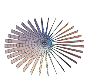
Figure 7: The standard radially-symmetric contact structure on $\mathbb{R}^{3}$. (Courtesy of the Mathematica routine ‘CSPlotter’ by Matias Dahl.)

We also require a few facts about Legendrian knots. By definition, ${C\subset{\mathbb{R}}^{3}}$ is Legendrian when the tangent line ${T_{p}C}$ at any point ${p\in C}$ lies in the contact plane $H_{p}$ at that point. Equivalently, the pullback of $\kappa$ to $C$ vanishes,

$$\kappa\big{|}_{C}\,=\,0\qquad\Longleftrightarrow\quad C\,\,\hbox{is Legendrian}\,,$$ (22)

or in terms of a parametrization ${X:S^{1}\to{\mathbb{R}}^{3}}$,

$$\frac{dz}{d\theta}\,=\,y\,\frac{dx}{d\theta}\,-\,x\,\frac{dy}{d\theta}\,,\qquad\qquad X(\theta)\equiv\big{(}x(\theta),\,y(\theta),\,z(\theta)\big{)}\,.$$ (23)

Any smooth knot admits a Legendrian representative, so the theory of Legendrian knots is extremely rich. Moreover, equivalence by Legendrian isotopy, ie. continuous isotopy through a family of Legendrian knots, strictly refines the usual topological equivalence. A given topological knot has infinitely-many inequivalent Legendrian representatives.

Unlike topological knots, Legendrian knots have canonical plane projections. For this reason, Legendrian knots behave in many ways like plane curves. Our interest lies in the so-called Lagrangian projection to the $xy$-plane,

$$\Pi:{\mathbb{R}}^{3}\,\to\,{\mathbb{R}}^{2}\,,\qquad\qquad\Pi(x,y,z)\,=\,(x,y)\,,$$ (24)

for which the image $\Pi(C)$ of a Legendrian knot ${C\subset{\mathbb{R}}^{3}}$ is a smoothly immersed curve. The smoothness of $\Pi(C)$ is already a non-trivial feature of the Legendrian condition (23), since this condition implies that ${\dot{z}=0}$ at any point on $C$ where ${\dot{x}=\dot{y}=0}$. Hence if $X$ is a regular parametrization of $C$, then ${\Pi\circ X}$ is a regular parametrization of $\Pi(C)$. Trivially, $\Pi(C)$ is a Lagrangian submanifold of ${\mathbb{R}}^{2}$ with respect to the symplectic form ${d\kappa=2\,dx{\wedge}dy}$, whence the name.

Figure 8: Legendrian trefoil knot, with ${\operatorname{\mathsf{tb}}(C)=1}$ and ${\operatorname{\mathsf{rot}}(C)=0}$.

In Figure 8 we display the Lagrangian projection of a Legendrian trefoil knot. To guide the eye, we indicate over- and under-crossings in the figure. Unlike for topological knot diagrams, the crossing information for a Legendrian knot is redundant, since the spatial configuration of ${C\subset{\mathbb{R}}^{3}}$ can be completely recovered from the plane curve $\Pi(C)$ by integrating the contact relation in (23),

$$z(\theta)\,=\,z_{0}\,+\,\int_{0}^{\theta}d\theta^{\prime}\left[y(\theta^{\prime})\,\dot{x}(\theta^{\prime})\,-\,x(\theta^{\prime})\,\dot{y}(\theta^{\prime})\right].$$ (25)

Here $z_{0}$ is the height of $C$ at the basepoint corresponding to ${\theta=0}$. Due the symmetry of $\kappa$ under translations in $z$, this constant is both arbitrary and irrelevant.

Not every immersed curve can be the plane projection of a Legendrian knot. For instance, if we take the parameter $\theta$ in (25) to have periodicity $2\pi$, then

$$0\,=\,z(2\pi)-z(0)\,=\,\int_{0}^{2\pi}d\theta^{\prime}\left[y(\theta^{\prime})\,\dot{x}(\theta^{\prime})\,-\,x(\theta^{\prime})\,\dot{y}(\theta^{\prime})\right].$$ (26)

Equivalently by Stokes’ Theorem, the oriented $2$-chain $D$ bounded by $\Pi(C)$ must have zero symplectic area,

$$\int_{D}dx{\wedge}dy\,=\,0\,,$$ (27)

where each component of $D$ is oriented consistently with ${\partial D=C}$. Also, if ${\theta_{1}\neq\theta_{2}}$ are distinct parameter values for which ${x(\theta_{1})=x(\theta_{2})}$ and ${y(\theta_{1})=y(\theta_{2})}$, corresponding to the location of a crossing in $\Pi(C)$, then

$$0\neq z(\theta_{2})-z(\theta_{1})\,=\,\int_{\theta_{1}}^{\theta_{2}}d\theta^{\prime}\left[y(\theta^{\prime})\,\dot{x}(\theta^{\prime})\,-\,x(\theta^{\prime})\,\dot{y}(\theta^{\prime})\right].$$ (28)

The necessary conditions in (26) and (28) are sufficient for the immersed plane curve to lift to an embedded Legendrian knot. These conditions depend upon the signed areas of the regions enclosed by $\Pi(C)$, so the Lagrangian projection cannot be manipulated in a wholly topological fashion á la Reidemeister.

Legendrian knots always carry a canonical framing by the Reeb vector field ${{\mathsf{R}}=\partial/\partial z}$. Concretely from (23), a Legendrian curve ${C\subset{\mathbb{R}}^{3}}$ cannot have a vertical tangent, where ${\dot{x}=\dot{y}=0}$ but ${\dot{z}\neq 0}$. With the choice ${n={\mathsf{R}}}$, the framed self-linking number $\operatorname{\mathsf{slk}}_{\rm f}(C,n)$ can then be converted into a Legendrian invariant

$$\operatorname{\mathsf{tb}}(C)\,:=\,\operatorname{\mathsf{slk}}_{\rm f}(C,{\mathsf{R}})\,\in\,{\mathbb{Z}}\,,$$ (29)

a kind of self-linking number for $C$.

The Thurston-Bennequin invariant $\operatorname{\mathsf{tb}}(C)$ can be easily computed from the Lagrangian projection of $C$. After a rigid rotation, the vertical framing by the Reeb field ${\mathsf{R}}$ becomes equivalent to the planar, blackboard framing of $\Pi(C)$. But again by Figure 6, the self-linking number in the blackboard framing is exactly the writhe of the knot diagram. Thus,

$$\operatorname{\mathsf{tb}}(C)\,=\,\operatorname{\mathsf{w}}\!\left(\Pi(C)\right).$$ (30)

Since the writhe is fixed under orientation-reversal, so too is

$$\operatorname{\mathsf{tb}}(-C)=\operatorname{\mathsf{tb}}(C)\,.$$ (31)

The Thurston-Bennequin invariant is one of a pair of classical Legendrian invariants. To state the Main Theorem, we also need the other.

Because $C$ is determined by its Lagrangian projection $\Pi(C)$, any isotopy invariant of immersed plane curves yields a Legendrian invariant of $C$. According to the Whitney-Graustein Theorem Whitney:1937 , the unique such invariant of an immersion ${\gamma:S^{1}\to{\mathbb{R}}^{2}}$ is the rotation number

$$\operatorname{\mathsf{rot}}(\gamma)\,=\,\deg\dot{\gamma}\,,\qquad\qquad\dot{\gamma}:S^{1}\to{\mathbb{R}}^{2}-\{0\}\,,$$ (32)

defined as the topological degree of the derivative $\dot{\gamma}$. Equivalently, $\operatorname{\mathsf{rot}}(\gamma)$ is the total signed curvature (see eg. Exercise 12 in §$1.5$ of doCarmo:76 ) of the immersed plane curve,

$$\operatorname{\mathsf{rot}}(\gamma)\,=\,\frac{1}{2\pi}\oint_{S^{1}}\!\!d\theta\,\,\frac{\dot{\gamma}\times\ddot{\gamma}}{||\dot{\gamma}||^{2}}\,,$$ (33)

where we use the shorthand ‘$\times$’ for the scalar cross-product,

$$\dot{\gamma}\times\ddot{\gamma}(\theta)\,\equiv\,\dot{x}(\theta)\,\ddot{y}(\theta)\,-\,\dot{y}(\theta)\,\ddot{x}(\theta)\,,\qquad\quad\gamma(\theta)=\left(x(\theta),y(\theta)\right)\in{\mathbb{R}}^{2}\,.$$ (34)

As will be essential later, the formula for $\operatorname{\mathsf{rot}}(\gamma)$ in (33) presents the rotation number as a local invariant, in the sense of being the integral of a locally-defined geometric quantity along the curve. With our conventions, ${\operatorname{\mathsf{rot}}(\gamma)=1}$ when $\gamma$ is a circle traversed in the counterclockwise direction.

For the Legendrian knot ${C\subset{\mathbb{R}}^{3}}$, we set

$$\operatorname{\mathsf{rot}}(C)\,:=\,\operatorname{\mathsf{rot}}\!\left(\Pi(C)\right)\in\,{\mathbb{Z}}\,.$$ (35)

See Definition $3.5.12$ in Geiges:2008 for an intrinsically three-dimensional characterization of $\operatorname{\mathsf{rot}}(C)$. In terms of the diagram for $\Pi(C)$, the rotation number can be computed as a signed count of upwards vertical tangencies, as in Figure 9. For the Legendrian trefoil in Figure 8, two upwards vertical tangencies occur, but they do so with opposite signs, so ${\operatorname{\mathsf{rot}}(C)=0}$.

Note that the rotation number depends upon the orientation of the curve, and under a reversal of orientation, the rotation number changes sign. So in contrast to the behavior (31) of the Thurston-Bennequin invariant,

$$\operatorname{\mathsf{rot}}(-C)\,=\,-\operatorname{\mathsf{rot}}(C)\,.$$ (36)

We have not specified an orientation for the trefoil knot in Figure 8, but because ${\operatorname{\mathsf{rot}}(C)=0}$, the orientation does not matter.

$$\begin{matrix}&\includegraphics[scale={0.50}]{rotp.eps}\qquad\quad&\quad\qquad&\includegraphics[scale={0.50}]{rotn.eps}\\ &(a.)\quad\operatorname{\mathsf{rot}}=+1\qquad\quad&\quad\qquad&(b.)\quad\operatorname{\mathsf{rot}}=-1\end{matrix}$$

Figure 9: Rotation number at upwards tangencies.

I.3 Main theorem

As its second consequence, supersymmetry modifies the angular form ${\psi\in\Omega^{2}\big{(}{\mathbb{R}}^{3}-\{0\}\big{)}}$ which enters the elementary Gauss linking integral (5). Because the Legendrian condition on ${C\subset{\mathbb{R}}^{3}}$ does not respect the Euclidean action by $SO(3)$, we forgo the seemingly-natural requirement that $\psi$ itself be $SO(3)$-invariant. In recompense, the supersymmetric version of $\psi$ will enjoy superior analytic behavior near the origin in ${\mathbb{R}}^{3}$.

As heuristic motivation for the following, one should imagine that we alter the angular form $\psi$ in (1) by concentrating the support for the generator of $H^{2}(S^{2};{\mathbb{Z}})$ at the North Pole on the sphere. This trick is well-known to aficionados of Chern-Simons perturbation theory, but here we must take care to preserve the underlying symmetries of the contact structure on ${\mathbb{R}}^{3}$.

More precisely, we introduce the Gaussian two-form ${\omega_{\Lambda}\in\Omega^{2}\big{(}{\mathbb{R}}^{2}\big{)}}$ on the $xy$-plane,

$$\omega_{\Lambda}\,=\,\frac{\Lambda}{2\pi}\,{\rm e}^{\,\!-\Lambda(x^{2}+y^{2})/2}\,dx{\wedge}dy\,,\qquad\qquad\Lambda>0\,.$$ (37)

Here $\Lambda$ is a positive real parameter which sets the width of the Gaussian, and in the limit ${\Lambda\to\infty}$, the Gaussian becomes a delta-function concentrated at the origin in ${\mathbb{R}}^{2}$. Clearly $\omega_{\Lambda}$ is invariant under rotations, and $\omega_{\Lambda}$ is normalized so that for all $\Lambda$,

$$\int_{{\mathbb{R}}^{2}}\omega_{\Lambda}\,=\,1\,.$$ (38)

The various factors of two in (37) are standard and could be absorbed into $\Lambda$ if desired.

Though the support of $\omega_{\Lambda}$ is not compact, $\omega_{\Lambda}$ decays very rapidly at infinity. At least morally, $\omega_{\Lambda}$ should be regarded as a generator for the compactly-supported cohomology ${H^{2}_{c}\big{(}{\mathbb{R}}^{2};{\mathbb{Z}}\big{)}\simeq{\mathbb{Z}}}$ of the plane, on the same footing as the unit-area form on the sphere. Because the normalization condition in (38) does not depend on $\Lambda$, neither does the cohomology class of $\omega_{\Lambda}$. Explicitly, a small computation shows

$$\frac{\partial\omega_{\Lambda}}{\partial\Lambda}\,=\,\frac{1}{2\pi}\left[1\,-\,\frac{\Lambda(x^{2}+y^{2})}{2}\right]{\rm e}^{\,\!-\Lambda\,(x^{2}+y^{2})/2}\,dx{\wedge}dy\,=\,d\alpha_{\Lambda}\,,$$ (39)

where

$$\alpha_{\Lambda}\,=\,\frac{1}{4\pi}\,{\rm e}^{\,\!-\Lambda(x^{2}+y^{2})/2}\left(x\,dy-y\,dx\right)\,\in\,\Omega^{1}\big{(}{\mathbb{R}}^{2}\big{)}.$$ (40)

The transgression form $\alpha_{\Lambda}$ will reappear in the proof of our Fundamental Lemma. In the meantime, note that $\alpha_{\Lambda}$ is also $SO(2)$-invariant, as required by the relation to $\omega_{\Lambda}$ in (39).

We next introduce the planar analogue for the retraction onto $S^{2}$ in (2). To preserve the parabolic scaling in (21), we consider the map ${\varrho_{+}:{\mathbb{R}}^{3}_{+}\to{\mathbb{R}}^{2}}$ defined on the upper half-space ${\mathbb{R}}^{3}_{+}$ by

$$\varrho_{+}(x,y,z)\,=\,\left(\frac{x}{\sqrt{z}},\,\frac{y}{\sqrt{z}}\right),\qquad\qquad z>0\,.$$ (41)

Trivially, the image of $\varrho_{+}$ is preserved under the scaling for which $x$ and $y$ have weight one and $z$ has weight two.

Using the planar retraction in (41), we pull the Gaussian form ${\omega_{\Lambda}\in\Omega^{2}({\mathbb{R}}^{2})}$ back to a new two-form

$$\chi_{\Lambda} =\,\varrho_{+}^{*}\omega_{\Lambda}\,,$$ (42)

$$=\,\frac{\Lambda}{2\pi z}{\rm e}^{\,\!-\Lambda(x^{2}+y^{2})/2z}\left[dx{\wedge}dy\,+\,\frac{1}{2}\left(x\,dy-y\,dx\right)\!{\wedge}\frac{dz}{z}\right],\qquad z>0\,.$$

By construction, $\chi_{\Lambda}$ is invariant under the parabolic scaling and the action of $SO(2)$, but not $SO(3)$.

Of course, $\chi_{\Lambda}$ strongly resembles the heat kernel for the Laplacian in two dimensions. As with the heat kernel, so long as ${x^{2}+y^{2}\neq 0}$, the expression in (42) vanishes smoothly as ${z\to 0}$ from above. To define $\chi_{\Lambda}$ on the entire punctured space ${{\mathbb{R}}^{3}-\{0\}}$, we simply extend by zero,

$$\chi_{\Lambda}\,=\,0\,,\qquad\qquad z\leq 0\,.$$ (43)

With this choice, ${\chi_{\Lambda}\in\Omega^{2}({\mathbb{R}}^{3}-\{0\})}$ is automatically closed away from $\{0\}$ and generates the cohomology ${H^{2}\big{(}{\mathbb{R}}^{3}-\{0\};{\mathbb{Z}}\big{)}}$. For instance, over the unit sphere ${S^{2}\subset{\mathbb{R}}^{3}}$,

$$\int_{S^{2}}\chi_{\Lambda}\,=\,\int_{S^{2}\cap{\mathbb{R}}^{3}_{+}}\mskip-10.0mu\chi_{\Lambda}\,=\,\int_{{\mathbb{R}}^{2}}\omega_{\Lambda}\,=\,1\,.$$ (44)

We have yet to incorporate the Heisenberg symmetry of the contact structure. In the elementary Gauss linking integral, the abelian structure of ${\mathbb{R}}^{3}$ as a vector space enters implicitly through the definition of the difference map $\Gamma$ in (4). To preserve instead the non-abelian symmetry by left-translation in ${{\mathbb{H}}\simeq{\mathbb{R}}^{3}}$, we consider a Heisenberg difference map ${\widehat{\Gamma}:{\mathbb{H}}\times{\mathbb{H}}\to{\mathbb{H}}}$, given by

$$\widehat{\Gamma}(X_{1},X_{2}) =\,\mu(X_{1}^{-1},\,X_{2})\,=\,\mu(-X_{1},X_{2})\,,\qquad\qquad X_{1,2}\,\in\,{\mathbb{H}}\,,$$ (45)

$$=\,\left(x_{2}-x_{1},\,y_{2}-y_{1},\,z_{2}-z_{1}+x_{1}y_{2}-x_{2}y_{1}\right).$$

Since $\mu$ is the Heisenberg multiplication, ${\widehat{\Gamma}(X_{1},X_{2})=X_{1}^{-1}\cdot X_{2}}$ in the usual shorthand. This combination of $X_{1}$ and $X_{2}$ is invariant under simultaneous left-multiplication,

$$\widehat{\Gamma}(g\cdot X_{1},g\cdot X_{2})=\widehat{\Gamma}(X_{1},X_{2})\,,\qquad\qquad g\,\in\,{\mathbb{H}}\,,$$ (46)

and we have selected the relative signs of $X_{1}$ and $X_{2}$ in (45) to agree with the convention for the abelian difference in (4).

Proposition I.1 (Heisenberg Linking)

Suppose ${C_{i}\subset{\mathbb{R}}^{3}}$ for ${i=1,2}$ are disjoint oriented curves, not necessarily Legendrian, with respective parametrizations ${X_{i}:S^{1}\to{\mathbb{R}}^{3}}$. Then

$$\operatorname{\mathsf{lk}}(C_{1},C_{2})\,=\,\int_{T^{2}}\left(X_{1}\times X_{2}\right)^{*}\!\widehat{\Gamma}^{*}\chi_{\Lambda}\,,\qquad\qquad\Lambda>0\,.$$ (47)

This proposition follows from the fact that the heat form $\chi_{\Lambda}$ is equivalent in cohomology to the global angular form $\psi$,

$$[\chi_{\Lambda}]\,=\,[\psi]\,\in\,H^{2}\big{(}{\mathbb{R}}^{3}-\{0\};{\mathbb{Z}}\big{)}\,.$$ (48)

Also, the Heisenberg difference $\widehat{\Gamma}$ in (45) is homotopic to the abelian difference $\Gamma$. To see this, set

$$\mu_{\hbar}(X_{1},X_{2})\,=\,\big{(}x_{1}+x_{2},\,y_{1}+y_{2},\,z_{1}+z_{2}-\hbar\left(x_{1}y_{2}-x_{2}y_{1}\right)\big{)}\,,\qquad\hbar\,\in\,[0,1]\,.$$ (49)

Then

$$\widehat{\Gamma}_{\hbar}(X_{1},X_{2})\,=\,\mu_{\hbar}\!\left(X_{1}^{-1},\,X_{2}\right)\,=\,\big{(}x_{2}-x_{1},\,y_{2}-y_{1},\,z_{2}-z_{1}+\hbar\,(x_{1}y_{2}-x_{2}y_{1})\big{)}$$ (50)

smoothly interpolates from the abelian to the Heisenberg difference as the Planck constant $\hbar$ ranges over the interval from ${\hbar=0}$ to ${\hbar=1}$.  $\square$

Though the angular form $\psi$ and the heat form $\chi_{\Lambda}$ agree in cohomology, they behave very differently near the origin in ${\mathbb{R}}^{3}$. This analytic distinction matters crucially for approaches to self-linking.

Let ${C\subset{\mathbb{R}}^{3}}$ be an oriented Legendrian curve, with regular parametrization ${X:S^{1}\to{\mathbb{R}}^{3}}$. By analogy to the naive Gauss self-linking integral in (10), we consider a new Heisenberg self-linking integral

$$\operatorname{\mathsf{slk}}_{\kappa}(C)\,:=\,\underset{\varepsilon\to 0}{\lim}\int_{T^{2}-\Delta(\varepsilon)}\left(X\times X\right)^{*}\!\widehat{\Gamma}_{\hbar}^{*}\,\chi_{\Lambda}\,,\qquad\quad\hbar\,\in\,[0,1]\,,\qquad\quad\Lambda>0\,.$$ (51)

The remainder of the article is devoted to the proof of the following Main Theorem.

Theorem I.2 (Legendrian Self-Linking)

The limit defining $\operatorname{\mathsf{slk}}_{\kappa}(C)$ exists. The value of $\operatorname{\mathsf{slk}}_{\kappa}(C)$ is independent of $\Lambda$ and depends only upon the Legendrian isotopy class of $C$. In terms of the Thurston-Bennequin invariant $\operatorname{\mathsf{tb}}(C)$ and the rotation number $\operatorname{\mathsf{rot}}(C)$,

$$\operatorname{\mathsf{slk}}_{\kappa}(C)\,=\,\begin{cases}\quad\operatorname{\mathsf{tb}}(C)-\operatorname{\mathsf{rot}}(C)\,,\qquad&\hbar\,\neq\,1\,,\\ \quad\operatorname{\mathsf{tb}}(C)\,,\qquad&\hbar\,=\,1\,.\end{cases}$$ (52)

Informally, the Main Theorem states that the framing anomaly for knots in bosonic Chern-Simons theory is absent in supersymmetric Chern-Simons theory. The corresponding statement for Seifert-fibered three-manifolds was observed previously in Beasley:2005vf . The Main Theorem is also consistent with results of Fuchs and Tabachnikov Fuchs:99a identifying $\operatorname{\mathsf{tb}}(C)$ and $\operatorname{\mathsf{rot}}(C)$ as the only order ${\leq 1}$ finite-type invariants of Legendrian knots.

The strategy of proof for Theorem I.2 is straightforward. We first demonstrate that $\operatorname{\mathsf{slk}}_{\kappa}(C)$ is independent of the parameter $\Lambda$ which sets the width of the Gaussian in $\chi_{\Lambda}$. For any ${\varepsilon>0}$, the derivative of $\operatorname{\mathsf{slk}}_{\kappa}(C)$ with respect to $\Lambda$ is given in terms of a boundary integral of the transgression form $\alpha_{\Lambda}$ in (40). The content of our Fundamental Lemma in Section II is to demonstrate that the potentially anomalous boundary contribution from $\alpha_{\Lambda}$ vanishes in the limit ${\varepsilon\to 0}$, due to the rapid decay of the heat kernel away from the diagonal.

In Section III we directly evaluate the self-linking integral in the limit ${\Lambda\to\infty}$. In this regime, the self-linking integrand is non-negligible only in the neighborhood of points on $T^{2}$ which map under the product ${X\times X}$ to pairs of points ${p,q\in C}$ that become coincident under the Lagrangian projection to the $xy$-plane, ie. ${\Pi(p)=\Pi(q)}$. Such points on $T^{2}$ correspond either to the preimage of crossings in $\Pi(C)$, or more trivially, to points on the diagonal ${\Delta\subset T^{2}}$. The local contribution from the crossings leads to the appearance of the Thurston-Bennequin invariant $\operatorname{\mathsf{tb}}(C)$, while the local contribution from the diagonal $\Delta$ leads to the appearance of the rotation number $\operatorname{\mathsf{rot}}(C)$ for ${\hbar\neq 1}$. At the special value ${\hbar=1}$, the Heisenberg symmetry of the integrand is restored, and the anomalous contribution from $\Delta$ vanishes.

The Legendrian condition is used crucially throughout the analysis. Invariance under Legendrian isotopy follows a postiori from the formula in (52).

Let us emphasize one striking feature of Theorem I.2, which is perhaps best appreciated after one works through the localization computation in Section III.1. Namely, since the coefficients of $\operatorname{\mathsf{tb}}(C)$ and $\operatorname{\mathsf{rot}}(C)$ in (52) are integers, so is the value of $\operatorname{\mathsf{slk}}_{\kappa}(C)$! The coefficient of $\operatorname{\mathsf{tb}}(C)$ is directly related to our normalization condition (44) on the heat form $\chi_{\Lambda}$, required to recover the usual linking number in Proposition I.1. Thus the coefficient of $\operatorname{\mathsf{tb}}(C)$ is fixed by fiat to unity. In contrast, the coefficient of $\operatorname{\mathsf{rot}}(C)$ is determined by a delicate calculation near the diagonal ${\Delta\subset T^{2}}$, so its integrality for all $\hbar$ is a non-trivial feature of the Legendrian self-linking integral.

From the physical perspective, integrality of $\operatorname{\mathsf{slk}}_{\kappa}(C)$ is necessary for gauge invariance as well as consistency with standard lore about non-renormalization and the infrared behavior of supersymmetric Yang-Mills-Chern-Simons theory. See §$2.3$ of Beasley:2015 for a discussion of this statement. However, on the principle that no integer appears by chance, a simple topological explanation for the integrality of ${\operatorname{\mathsf{slk}}_{\kappa}(C)\in{\mathbb{Z}}}$ would be nice to have.

For instance, the difference of classical Legendrian invariants ${\operatorname{\mathsf{tb}}(C)-\operatorname{\mathsf{rot}}(C)}$ in (52) occurs naturally in contact topology as the transverse self-linking invariant $\operatorname{\mathsf{slk}}(C_{+})$ of the canonical positive transverse push-off $C_{+}$ of $C$ (Proposition $3.5.36$ in Geiges:2008 ). The transverse self-linking invariant $\operatorname{\mathsf{slk}}(C_{+})$ can be interpreted in terms of a relative Euler class on a Seifert surface for $C_{+}$, so its appearance in Theorem I.2 is surely no accident.

I.4 Notation and conventions

For the convenience of the reader, we summarize the notation and conventions used in the rest of the paper.

• ${\mathbb{R}}^{3}$ has Euclidean coordinates $(x,y,z)$ and is oriented by ${dx{\wedge}dy{\wedge}dz}$.

• The map ${\Pi:{\mathbb{R}}^{3}\to{\mathbb{R}}^{2}}$ is the projection onto the $xy$-plane.

• ${\kappa=dz+x\,dy-y\,dx}$ is the standard radially-symmetric contact form, positive with respect to the orientation on ${\mathbb{R}}^{3}$.

• ${C\subset{\mathbb{R}}^{3}}$ is an oriented Legendrian knot, with regular parametrization ${X:S^{1}\to{\mathbb{R}}^{3}}$.

• ${\theta\sim\theta+2\pi}$ is an angular coordinate on $S^{1}$, compatible under $X$ with the given orientation on $C$. We abbreviate ${dX/d\theta\equiv\dot{X}(\theta)}$, and so on.

• The torus ${T^{2}=S^{1}\times S^{1}}$ has angular coordinates $(\theta_{1},\theta_{2})$ and is oriented by ${d\theta_{1}{\wedge}d\theta_{2}}$. The diagonal ${\Delta\subset T^{2}}$ is the subset where ${\theta_{1}=\theta_{2}}$.

• For ${\varepsilon>0}$, a tubular neighborhood $\Delta(\varepsilon)$ of the diagonal ${\Delta\subset T^{2}}$ is parametrized by ${\theta_{1}=\phi}$ and ${\theta_{2}=\phi+\eta}$ for ${|\eta|<\varepsilon}$. The cylinder ${T^{2}-\Delta(\varepsilon)}$ has boundary circles $S^{1}_{\pm}$ on which ${\eta=\pm\varepsilon}$, respectively.

• ${\gamma:S^{1}\to{\mathbb{R}}^{2}}$ is an immersed plane curve which is the Lagrangian projection of $C$, ie. ${\gamma=\Pi\circ X}$.

• We use the abbreviation ‘$\times$’ for the scalar cross-product on the plane, as in

  $$\gamma\times\dot{\gamma}(\theta)\,\equiv\,x(\theta)\,\dot{y}(\theta)\,-\,y(\theta)\,\dot{x}(\theta)\,,\qquad\quad\gamma(\theta)=\left(x(\theta),y(\theta)\right)\in{\mathbb{R}}^{2}\,.$$

• The contact form $\kappa$ is left-invariant with respect to the Heisenberg multiplication

  $$\mu:{\mathbb{H}}\times{\mathbb{H}}\to{\mathbb{H}}\,,\qquad\qquad{\mathbb{H}}\simeq{\mathbb{R}}^{3}\,,\qquad\qquad[\hbar=1]$$

  $$\mu\big{(}X_{1},X_{2}\big{)}\,=\,\left(x_{1}+x_{2},\,y_{1}+y_{2},\,z_{1}+z_{2}-x_{1}y_{2}+x_{2}y_{1}\right).$$

  More generally, for other values of $\hbar$ set

  $$\mu_{\hbar}(X_{1},X_{2})\,=\,\big{(}x_{1}+x_{2},\,y_{1}+y_{2},\,z_{1}+z_{2}-\hbar\left(x_{1}y_{2}-x_{2}y_{1}\right)\big{)}\,.$$

• The left-invariant Heisenberg difference ${\widehat{\Gamma}_{\hbar}:{\mathbb{H}}\times{\mathbb{H}}\to{\mathbb{H}}}$ for ${\hbar\in[0,1]}$ is given by

  $$\widehat{\Gamma}_{\hbar}(X_{1},X_{2}) =\,\mu_{\hbar}(X_{1}^{-1},\,X_{2})\,,$$

  $$=\,\left(x_{2}-x_{1},\,y_{2}-y_{1},\,z_{2}-z_{1}+\hbar\left(x_{1}y_{2}-x_{2}y_{1}\right)\right).$$

• The Gaussian fundamental class ${\omega_{\Lambda}\in\Omega^{2}\big{(}{\mathbb{R}}^{2}\big{)}}$ of the $xy$-plane is given by

  $$\omega_{\Lambda}\,=\,\frac{\Lambda}{2\pi}\,{\rm e}^{\,\!-\Lambda(x^{2}+y^{2})/2}\,dx{\wedge}dy\,,\qquad\qquad\Lambda>0\,.$$

• The transgression form ${\alpha_{\Lambda}\in\Omega^{1}\big{(}{\mathbb{R}}^{2}\big{)}}$ satisfies ${\partial\omega/\partial\Lambda=d\alpha_{\Lambda}}$, where

  $$\alpha_{\Lambda}\,=\,\frac{1}{4\pi}\,{\rm e}^{\,\!-\Lambda(x^{2}+y^{2})/2}\left(x\,dy-y\,dx\right).$$

• The planar retraction ${\varrho_{+}\!:{\mathbb{R}}^{3}_{+}\to{\mathbb{R}}^{2}}$ is defined on the upper half-space ${\mathbb{R}}^{3}_{+}$ by

  $$\varrho_{+}(x,y,z)\,=\,\left(\frac{x}{\sqrt{z}},\,\frac{y}{\sqrt{z}}\right),\qquad\qquad z>0\,.$$

• The heat form ${\chi_{\Lambda}\in\Omega^{2}\big{(}{\mathbb{R}}^{3}-\{0\}\big{)}}$ is the pullback

  $$\chi_{\Lambda}\,=\,\begin{cases}\qquad\varrho_{+}^{*}\omega_{\Lambda},\qquad&z>0\,,\\ \qquad 0\,,\qquad&z\leq 0\,.\end{cases}$$

  Explicitly,

  $$\varrho_{+}^{*}\omega_{\Lambda}\,=\,\frac{\Lambda}{2\pi z}{\rm e}^{\,\!-\Lambda(x^{2}+y^{2})/2z}\left[dx{\wedge}dy\,+\,\frac{1}{2}\left(x\,dy-y\,dx\right)\!{\wedge}\frac{dz}{z}\right],\qquad z>0\,.$$

II Fundamental lemma

We first demonstrate that the value of the Legendrian self-linking integral $\operatorname{\mathsf{slk}}_{\kappa}(C)$ does not depend upon the parameter ${\Lambda>0}$ which sets the width of the Gaussian in the heat form $\chi_{\Lambda}$.

Lemma II.1 (Fundamental Lemma)

The limit which defines the Legendrian self-linking integral $\operatorname{\mathsf{slk}}_{\kappa}(C)$ exists,

$$\operatorname{\mathsf{slk}}_{\kappa}(C)\,=\,\underset{\varepsilon\to 0}{\lim}\int_{T^{2}-\Delta(\varepsilon)}\left(X\times X\right)^{*}\!\widehat{\Gamma}^{*}_{\hbar}\,\chi_{\Lambda}\,,\qquad\quad\hbar\,\in\,[0,1]\,,\qquad\quad\Lambda>0\,,$$ (53)

and the value of ${\operatorname{\mathsf{slk}}_{\kappa}(C)\in{\mathbb{R}}}$ is independent of the parameter $\Lambda$.

Precisely at the special value ${\hbar=1}$, the self-linking integrand is Heisenberg-invariant. For this reason, the analysis to prove Lemma II.1 will differ slightly depending on whether ${\hbar\neq 1}$ or ${\hbar=1}$.

Throughout, we make two extra topological assumptions about the Legendrian knot $C$. Both assumptions hold generically and help to simplify the proofs.

1. The Lagrangian projection $\Pi(C)$ is an immersed plane curve $\gamma$ with only double-point singularities, as in Figure 8.

2. The height function $z(\theta)$ on ${C\subset{\mathbb{R}}^{3}}$ is Morse, with isolated non-degenerate critical points. That is, $\dot{z}$ vanishes only at isolated points ${p\in C}$, at which ${\ddot{z}\neq 0}$. Because $C$ is Legendrian, the Morse condition on $z(\theta)$ is equivalent by (23) to the condition that the function ${\gamma\times\dot{\gamma}}$ vanish only at isolated points ${\theta\in S^{1}}$, at which ${\gamma\times\ddot{\gamma}\neq 0}$.

The first assumption is standard. Otherwise, the Morse condition is used only in the case ${\hbar\neq 1}$ and could possibly be relaxed, at the cost of further effort.

Before embarking on the proof of our Fundamental Lemma, let us mention an easy corollary which is handy for the gauge theory analysis in §$5$ of Beasley:2015 . To state the corollary, we require additional notation. Let ${t>0}$ be a positive scaling parameter. As in the remarks following Proposition I.1, we consider a version of the Heisenberg difference $\widehat{\Gamma}_{t\hbar}$ with rescaled Planck constant ${t\hbar}$ for fixed ${\hbar\in[0,1]}$,

$$\widehat{\Gamma}_{t\hbar}(X_{1},X_{2})\,=\,\left(x_{2}-x_{1},\,y_{2}-y_{1},\,z_{2}-z_{1}+t\hbar\left(x_{1}y_{2}-x_{2}y_{1}\right)\right).$$ (54)

For each value of $t$, we associate the contact form

$$\kappa_{t}\,=\,t^{-1/2}\,dz\,+\,t^{1/2}\left(x\,dy-y\,dx\right).$$ (55)

The relative power of $t$ between the two terms in (55) ensures that the contact form is left-invariant under the Heisenberg multiplication with ${\hbar=t}$ in (49). The overall power of $t$ ensures that the contact condition ${\kappa_{t}{\wedge}d\kappa_{t}=2\,dx{\wedge}dy{\wedge}dz\neq 0}$ is satisfied trivially for all values ${t>0}$.

Finally, suppose that ${C\subset{\mathbb{R}}^{3}}$ is a Legendrian knot with respect to the standard contact form $\kappa_{t=1}$. Just as we consider the family of isotopic contact forms in (55), we would like to consider a family of isotopic knots ${C_{t}\subset{\mathbb{R}}^{3}}$, each of which is Legendrian with respect to $\kappa_{t}$ for the given value of $t$. Such a family of knots is determined if we simply require the Lagrangian projection of $C_{t}$ to coincide with that of $C$,

$$\Pi(C_{t})\,=\,\Pi(C)\,,\qquad\qquad t\,>\,0\,.$$ (56)

Either by integrating the contact condition as in (25) or just by scaling, the embedding map ${X_{t}\!:S^{1}\to{\mathbb{R}}^{3}}$ for $C_{t}$ is then related to the original embedding $X$ for $C$ via

$$X_{t}(\theta)\,\equiv\left(x_{t}(\theta),\,y_{t}(\theta),\,z_{t}(\theta)\right)=\left(x(\theta),\,y(\theta),\,t\,z(\theta)\right).$$ (57)

In particular, the abelian limit ${t\to 0}$ of the Heisenberg structure corresponds to a limit in which $C_{t}$ flattens to a curve in the $xy$-plane, and the Lagrangian projection $\Pi(C)$ is realized geometrically.

Given the family of curves $C_{t}$, we consider the three-parameter self-linking integral

$$\operatorname{\mathsf{slk}}_{\kappa}(C_{t})\,=\,\underset{\varepsilon\to 0}{\lim}\int_{T^{2}-\Delta(\varepsilon)}\left(X_{t}\times X_{t}\right)^{*}\!\widehat{\Gamma}_{t\hbar}^{*}\,\chi_{\Lambda}\,,\qquad\quad\hbar\in[0,1]\,,\qquad\quad t,\Lambda>0\,.$$ (58)

Precisely for ${\hbar=1}$, the self-linking integrand is invariant under the Heisenberg symmetry with multiplication map $\mu_{t}$.

Remark II.2 (Scaling Identity)

For all ${t,\Lambda>0}$,

$$\left(X_{t}\times X_{t}\right)^{*}\!\widehat{\Gamma}_{t\hbar}^{*}\,\chi_{\Lambda}\,=\,\left(X\times X\right)^{*}\!\widehat{\Gamma}_{\hbar}^{*}\,\chi_{\Lambda/t}\,.$$ (59)

By the Scaling Identity, the behavior of the self-linking integrand in limit ${\Lambda\to\infty}$ with fixed $t$ is the same as the behavior in the limit ${t\to 0}$ with fixed $\Lambda$. Because $C_{t}$ flattens to a plane curve in the latter limit, $\Lambda$ plays a similar role to the parameter of the same name in (16).

Proof of Scaling Identity The $t$-dependence of the pullback is $\left(X_{t}\times X_{t}\right)^{*}\!\widehat{\Gamma}_{t\hbar}^{*}\,\chi_{\Lambda}$ is actually very simple. In terms of the finite differences

$$\Delta x\,=\,x_{2}-x_{1}\,,\qquad\quad\Delta y\,=\,y_{2}-y_{1}\,,\qquad\quad\widehat{\Delta}z\,=\,z_{2}-z_{1}+\hbar\left(x_{1}y_{2}-x_{2}y_{1}\right),$$ (60)

the formula for the heat form $\chi_{\Lambda}$ in (42) implies

$$\left(X_{t}\times X_{t}\right)^{*}\!\widehat{\Gamma}_{t\hbar}^{*}\,\chi_{\Lambda}\,=\,$$ (61)

$$\qquad\frac{\Lambda}{2\pi t\widehat{\Delta}z}\,{\rm e}^{\,\!-\Lambda(\Delta x^{2}+\Delta y^{2})/2t\widehat{\Delta}z}\left[d\Delta x{\wedge}d\Delta y\,+\frac{1}{2}\left(\Delta x\,d\Delta y-\Delta y\,d\Delta x\right)\!{\wedge}\frac{d\widehat{\Delta}z}{\widehat{\Delta}z}\right],$$

provided ${\widehat{\Delta}z>0}$. Otherwise, the pullback of $\chi_{\Lambda}$ vanishes. Evidently, $t$ just multiplies $\widehat{\Delta}z$ in (61), and all dependence on $t$ can be absorbed by rescaling the Gaussian parameter $\Lambda$.  $\square$

Corollary II.3

The value of $\operatorname{\mathsf{slk}}_{\kappa}(C_{t})$ in (58) is independent of both $t$ and $\Lambda$.

Proof The corollary follows immediately from Lemma II.1 and the Scaling Identity in (59).  $\square$

II.1 Analysis near the diagonal

The non-trivial aspect of our work concerns the local analysis of the self-linking integrand in the vicinity of the diagonal ${\Delta\subset T^{2}}$. In practice, this analysis amounts to the Taylor expansion of expressions such as occur in (61). Rather than scatter such expansions willy-nilly throughout the paper, we collect here the basic ingredients to be used again and again.

Let $(\theta_{1},\theta_{2})$ be angular coordinates on $T^{2}$. To parametrize the tubular neighborhood ${\Delta(\varepsilon)\subset T^{2}}$ of the diagonal, we set

$$\theta_{1}\,=\,\phi\,,\qquad\qquad\theta_{2}\,=\,\phi+\eta\,.$$ (62)

Here $\phi$ is an angular coordinate along the diagonal, and $\Delta(\varepsilon)$ is the subset where ${|\eta|<\varepsilon}$. Our local expansions near the diagonal will then be Taylor expansions in $\eta$, appropriate for the regime ${\varepsilon\ll 1}$. We must be careful about orientations. In terms of the coordinates $(\phi,\eta)$, the orientation form on $T^{2}$ is given by ${d\theta_{1}{\wedge}d\theta_{2}=d\phi{\wedge}d\eta}$. Topologically, the configuration space ${T^{2}-\Delta(\varepsilon)}$ is a cylinder with oriented boundary circles

$$S^{1}_{\pm}:\quad\eta\,=\,\pm\varepsilon\mod 2\pi\,.$$ (63)

As shown in Figure 10, the boundary orientation of $S^{1}_{+}$ is positive with respect to the direction of increasing $\phi$ and the orientation of $S^{1}_{-}$ is negative, so

$$\partial\!\left(T^{2}-\Delta(\varepsilon)\right)\,=\,S^{1}_{+}\,-\,S^{1}_{-}\,.$$ (64)

Figure 10: Orientations on the cylinder ${T^{2}-\Delta(\varepsilon)}$.

We now expand the various terms appearing in the self-linking integrand ${(X\times X)^{*}\widehat{\Gamma}_{\hbar}^{*}\,\chi_{\Lambda}}$, given by the expression in (61) for ${t=1}$. We start with

$$\Delta x\,=\,x(\theta_{2})-x(\theta_{1})\,=\,x(\phi+\eta)-x(\phi)\,=\,\eta\,\dot{x}(\phi)\,+\,{\mathcal{O}}\big{(}\varepsilon^{2}\big{)}\,,$$ (65)

and similarly for $\Delta y$. Hence

$$\Delta x^{2}+\Delta y^{2}\,=\,\eta^{2}\left(\dot{x}^{2}+\dot{y}^{2}\right)\,+\,{\mathcal{O}}\big{(}\varepsilon^{3}\big{)}\,=\,\eta^{2}\,||\dot{\gamma}||^{2}\,+\,{\mathcal{O}}\big{(}\varepsilon^{3}\big{)}\,,$$ (66)

where ${\gamma(\phi)=\left(x(\phi),y(\phi)\right)}$ is the Lagrangian immersion ${\gamma=\Pi\circ X}$ as before. For the related two-form, we can write

$$d\Delta x{\wedge}d\Delta y =\,\frac{1}{2}\,d\Delta\gamma\times d\Delta\gamma\,,\qquad\qquad\qquad\Delta\gamma\equiv\left(\Delta x,\Delta y\right),$$ (67)

$$=\,\frac{1}{2}\,d(\eta\,\dot{\gamma})\times d(\eta\,\dot{\gamma})\,+\,{\mathcal{O}}\big{(}\varepsilon^{3}\big{)}\,,$$

$$=\,\frac{1}{2}\left(\dot{\gamma}\,d\eta\,+\,\eta\,\ddot{\gamma}\,d\phi\right)\times\left(\dot{\gamma}\,d\eta\,+\,\eta\,\ddot{\gamma}\,d\phi\right)\,+\,{\mathcal{O}}\big{(}\varepsilon^{3}\big{)}.$$

After collecting terms in the product,

$$d\Delta x{\wedge}d\Delta y\,=\,-\eta\,\left(\dot{\gamma}\times\ddot{\gamma}\right)d\phi{\wedge}d\eta\,+\,{\mathcal{O}}\big{(}\varepsilon^{2}\big{)}\,d\phi{\wedge}d\eta\,.$$ (68)

Recall the definition

$$\widehat{\Delta}z\,=\,z_{2}-z_{1}+\hbar\left(x_{1}y_{2}-x_{2}y_{1}\right).$$ (69)

The Legendrian condition on $C$ is absolutely critical for our results, because it implies that the local behavior of $\widehat{\Delta}z$ near the diagonal is controlled by the geometry of the Lagrangian immersion $\gamma$. Moreover, the quadratic terms in $\widehat{\Delta}z$ are required by the Heisenberg symmetry when ${\hbar=1}$.

The expansion of the abelian difference ${\Delta z=z_{2}-z_{1}}$ is fixed by the Legendrian condition

$$\dot{z}\,=\,y\,\dot{x}\,-\,x\,\dot{y}\,=\,-\gamma\times\dot{\gamma}\,.$$ (70)

Thus

$$z_{2}-z_{1} =\,z(\phi+\eta)-z(\phi)\,=\,\eta\,\dot{z}(\phi)\,+\,\frac{1}{2}\,\eta^{2}\,\ddot{z}(\phi)\,+\,\frac{1}{6}\,\eta^{3}\,\dddot{z}(\phi)\,+\,{\mathcal{O}}\big{(}\varepsilon^{4}\big{)}\,,$$ (71)

$$=\,-\eta\left(\gamma\times\dot{\gamma}\right)\,-\,\frac{1}{2}\,\eta^{2}\left(\gamma\times\ddot{\gamma}\right)\,-\,\frac{1}{6}\,\eta^{3}\left(\dot{\gamma}\times\ddot{\gamma}\,+\,\gamma\times\dddot{\gamma}\right)\,+\,{\mathcal{O}}\big{(}\varepsilon^{4}\big{)}\,.$$

In passing to the second line of (71), we repeatedly differentiate the Legendrian condition on $\dot{z}$ in (70).

The attentive reader may wonder why we have expanded ${\Delta z=z_{2}-z_{1}}$ all the way to cubic order in $\eta$. The question answers itself once we expand the remaining quadratic terms in the Heisenberg difference $\widehat{\Delta}z$,

$$x_{1}y_{2}-x_{2}y_{1} =\,\gamma(\phi)\times\gamma(\phi+\eta)\,,$$ (72)

$$=\,\eta\left(\gamma\times\dot{\gamma}\right)\,+\,\frac{1}{2}\,\eta^{2}\left(\gamma\times\ddot{\gamma}\right)\,+\,\frac{1}{6}\,\eta^{3}\left(\gamma\times\dddot{\gamma}\right)\,+\,{\mathcal{O}}\big{(}\varepsilon^{4}\big{)}\,.$$

So long as ${\hbar\neq 1}$, the expansion of $\widehat{\Delta}z$ begins at linear order in $\eta$,

$$\widehat{\Delta}z\,\buildrel\hbar\neq 1\over{=}\,-\eta\left(1-\hbar\right)\left(\gamma\times\dot{\gamma}\right)\,+\,{\mathcal{O}}\big{(}\varepsilon^{2}\big{)}\,,$$ (73)

as one naively expects. But precisely at ${\hbar=1}$, cancellations occur in the sum of (71) and (72), and the leading term in the expansion of $\widehat{\Delta}z$ near the diagonal begins at cubic order,

$$\widehat{\Delta}z\,\buildrel\hbar=1\over{=}\,-\frac{1}{6}\eta^{3}\left(\dot{\gamma}\times\ddot{\gamma}\right)+\,{\mathcal{O}}\big{(}\varepsilon^{4}\big{)}\,.$$ (74)

The cancellation in (74) is forced by the Heisenberg symmetry at ${\hbar=1}$. Clearly, the quantity ${\gamma\times\dot{\gamma}}$ in (73) is not invariant under translations ${\gamma\mapsto\gamma+\gamma_{0}}$ for constant ${\gamma_{0}\in{\mathbb{R}}^{2}}$. Upon projection to the $xy$-plane, such translations are generated by the Heisenberg action, so ${\gamma\times\dot{\gamma}}$ is forbidden to appear at ${\hbar=1}$.

Combining the expansions in (66), (73), and (74), we see that the argument of the heat kernel is given in the neighborhood $\Delta(\varepsilon)$ by

$$\frac{\Delta x^{2}+\Delta y^{2}}{2\widehat{\Delta}z}\,=\,\Bigg{\{}\quad\begin{aligned} &-\frac{||\dot{\gamma}||^{2}\,\eta}{2\left(1-\hbar\right)\left(\gamma\times\dot{\gamma}\right)}\,+\,{\mathcal{O}}\big{(}\varepsilon^{2}\big{)}\,,\qquad&\hbox{\small$[\hbar\neq 1]$}\\[4.30554pt] &-\frac{3\,||\dot{\gamma}||^{2}}{\left(\dot{\gamma}\times\ddot{\gamma}\right)\eta}\,+\,{\mathcal{O}}(1)\,.&\hbox{\small$[\hbar=1]$}\end{aligned}$$ (75)

For generic ${\hbar\neq 1}$, the argument of the heat kernel in (75) vanishes linearly near the diagonal. However, at the symmetric point ${\hbar=1}$, the argument instead diverges as ${\eta\to 0}$. In Section III, this difference will ultimately lead to the discontinuity in the value of $\operatorname{\mathsf{slk}}_{\kappa}(C)$ at ${\hbar=1}$.

Remark II.4 (Local Positivity)

The pullback of the heat form $\chi_{\Lambda}$ vanishes identically unless ${\widehat{\Delta}z>0}$. On the neighborhood $\Delta(\varepsilon)$, positivity of $\widehat{\Delta}z$ becomes equivalent via (73) and (74) to the local sign condition

$$\widehat{\Delta}z\big{|}_{\Delta(\varepsilon)}>0\quad\Longleftrightarrow\quad\Bigg{\{}\begin{aligned} &\eta\left(1-\hbar\right)\left(\gamma\times\dot{\gamma}\right)<0\,,\qquad&\hbox{\small$[\hbar\neq 1]$}\,,\\ &\eta\left(\dot{\gamma}\times\ddot{\gamma}\right)<0\,.&\hbox{\small$[\hbar=1]$}\,.\end{aligned}$$ (76)

Again, the nature of the positivity condition depends upon whether or not ${\hbar=1}$. For generic values of $\hbar$, the sign of $\eta$ is determined by the sign of $\gamma\times\dot{\gamma}$ and hence the sign of the derivative $\dot{z}$. For ${\hbar=1}$, the sign of $\eta$ is instead fixed by the sign of $\dot{\gamma}\times\ddot{\gamma}$, proportional to the plane curvature of $\Pi(C)$.

$$\begin{matrix}&\includegraphics[scale={0.60}]{etap.eps}\quad\qquad&\quad\qquad&\includegraphics[scale={0.60}]{etan.eps}\\[4.30554pt] &(a.)\quad\eta>0\,,\,\dot{\gamma}\times\ddot{\gamma}<0\quad\qquad&\quad\qquad&(b.)\quad\eta<0\,,\,\dot{\gamma}\times\ddot{\gamma}>0\end{matrix}$$

Figure 11: Local positivity condition ${\widehat{\Delta}z>0}$ for ${\hbar=1}$.

Since the local positivity condition depends upon the sign of $\eta$, the self-linking integrand always vanishes in the neighborhood of one or the other of the boundary circles $S^{1}_{\pm}$ in Figure 10, and the geometry of $C$ at any given point determines on which boundary circle the integrand vanishes. See Figure 11 for a geometric illustration of the local positivity condition ${\widehat{\Delta}z>0}$ in the symmetric case ${\hbar=1}$. For clarity, we exaggerate the small separation between the points $\gamma(\theta_{1})$ and $\gamma(\theta_{2})$ in the figure. In both cases, the positivity condition is sensitive to the orientation of $C$, as a reversal of orientation flips the signs of $\gamma\times\dot{\gamma}$ and $\dot{\gamma}\times\ddot{\gamma}$ in (76).

Let us complete the expansion for small $\eta$ of the self-linking integrand. The second bracketed term in (61) involves the angular one-form

$$\Delta x\,d\Delta y\,-\,\Delta y\,d\Delta x =\,\Delta\gamma\times d\Delta\gamma\,,$$ (77)

$$=\,\left(\eta\,\dot{\gamma}\right)\times d\left(\eta\,\dot{\gamma}\right)+{\mathcal{O}}\big{(}\varepsilon^{3}\big{)}\,,$$

$$=\,\eta^{2}\left(\dot{\gamma}\times\ddot{\gamma}\right)d\phi\,+\,{\mathcal{O}}\big{(}\varepsilon^{3}\big{)}\,.$$

From the expansions of ${\widehat{\Delta}z}$ in (73) and (74),

$$\left(\Delta x\,d\Delta y-\Delta y\,d\Delta x\right)\!{\wedge}d\widehat{\Delta}z=\Bigg{\{}\begin{aligned} &-\left(1-\hbar\right)\left(\gamma\times\dot{\gamma}\right)\left(\dot{\gamma}\times\ddot{\gamma}\right)\eta^{2}\,d\phi{\wedge}d\eta\,,\quad&\hbox{\small$[\hbar\neq 1]$}\\ &-\frac{1}{2}\left(\dot{\gamma}\times\ddot{\gamma}\right)^{2}\eta^{4}\,d\phi{\wedge}d\eta\,,&\hbox{\small$[\hbar=1]$}\end{aligned}$$ (78)

to leading order, so

$$\left(\Delta x\,d\Delta y-\Delta y\,d\Delta x\right)\!{\wedge}\frac{d\widehat{\Delta}z}{\widehat{\Delta}z}=\Bigg{\{}\begin{aligned} &\eta\left(\dot{\gamma}\times\ddot{\gamma}\right)d\phi{\wedge}d\eta\,+\,{\mathcal{O}}\big{(}\varepsilon^{2}\big{)}\,d\phi{\wedge}d\eta\,,\qquad&\hbox{\small$[\hbar\neq 1]$}\\ &3\,\eta\left(\dot{\gamma}\times\ddot{\gamma}\right)d\phi{\wedge}d\eta\,+\,{\mathcal{O}}\big{(}\varepsilon^{2}\big{)}\,d\phi{\wedge}d\eta\,.&\hbox{\small$[\hbar=1]$}\end{aligned}$$ (79)

After a bit of algebra, one finds that the pullback (61) of $\chi_{\Lambda}$ behaves near the diagonal ${\Delta\subset T^{2}}$ for ${\hbar\neq 1}$ as

$$\left(X\times X\right)^{*}\!\widehat{\Gamma}_{\hbar}^{*}\,\chi_{\Lambda}\Big{|}_{\Delta(\varepsilon)}\buildrel\hbar\neq 1\over{=}$$ (80)

$$\qquad-\operatorname{\mathrm{sgn}}(\eta)\,\frac{\Lambda\left(\dot{\gamma}\times\ddot{\gamma}\right)}{4\pi\,|1-\hbar|\,|\gamma\times\dot{\gamma}|}\,\exp{\!\left[-\frac{\Lambda\,||\dot{\gamma}||^{2}\,|\eta|}{2\,|1-\hbar|\,|\gamma\times\dot{\gamma}|}\right]}\,d\phi{\wedge}d\eta\,+\,\cdots\,,$$

assuming the sign condition ${\eta\left(1-\hbar\right)\left(\gamma\times\dot{\gamma}\right)<0}$ in (76) holds. Otherwise, the pullback is equal to zero. The sign condition ensures that the exponential in (80) is always decaying, and it leads to a non-analytic dependence on the sign of $\eta$. The ellipses in (80) indicate subleading terms which vanish as ${\eta\to 0}$.

By contrast, at the symmetric value ${\hbar=1}$,

$$\left(X\times X\right)^{*}\!\widehat{\Gamma}^{*}_{\hbar}\,\chi_{\Lambda}\Big{|}_{\Delta(\varepsilon)} \buildrel\hbar=1\over{=}\,-\frac{3\,\Lambda}{2\pi\eta^{2}}\exp{\!\left[-\frac{3\,\Lambda\,||\dot{\gamma}||^{2}}{\left|\dot{\gamma}\times\ddot{\gamma}\right|}\frac{1}{|\eta|}\right]}\,d\phi{\wedge}d\eta\,+\,\cdots\,,$$ (81)

$$\,=\,\frac{3\,\Lambda}{2\pi}\exp{\!\left[-\frac{3\,\Lambda\,||\dot{\gamma}||^{2}}{\left|\dot{\gamma}\times\ddot{\gamma}\right|}\,|\nu|\right]}\,d\phi{\wedge}d\nu\,+\,\cdots\,,$$

under the sign condition ${\eta\left(\dot{\gamma}\times\ddot{\gamma}\right)<0}$ in (76). In passing to the second line, we make the substitution ${\nu=1/\eta}$ for clarity. In this case, the pullback of the heat form $\chi_{\Lambda}$ vanishes exponentially as ${|\nu|\to\infty}$, or equivalently ${|\eta|\to 0}$.

II.2 Proof of the fundamental lemma

The proof of our Fundamental Lemma II.1 is now an exercise in calculus.

As a brief formality, we first establish that the singularity in the pullback of the heat form $\chi_{\Lambda}$ is integrable, so that the defining limit ${\varepsilon\to 0}$ in (53) does exist. By assumption, ${||\dot{\gamma}||^{2}>0}$ is everywhere non-vanishing, and the functions $|\gamma\times\dot{\gamma}|$ and $|\dot{\gamma}\times\ddot{\gamma}|$ are bounded from above on $C$. Integrability in the region of small ${|\eta|<\varepsilon}$ follows immediately from the local expressions in (80) and (81), both of which remain finite as ${\eta\to 0}$.

Otherwise, we must check that the value of $\operatorname{\mathsf{slk}}_{\kappa}(C)$ does not depend upon the parameter ${\Lambda>0}$. This argument will be equally straightforward but the result is significant; the analogue for the naive Gauss self-linking integral $\operatorname{\mathsf{slk}}_{0}(C)$ is simply false. Our strategy will be to show that the derivative of $\operatorname{\mathsf{slk}}_{\kappa}(C)$ with respect to $\Lambda$ vanishes for all values of ${\Lambda>0}$. The details differ somewhat depending upon whether ${\hbar\neq 1}$ or ${\hbar=1}$, but the main idea is the same in both cases.

We compute

$$\frac{d\operatorname{\mathsf{slk}}_{\kappa}(C)}{d\Lambda} =\,\underset{\varepsilon\to 0}{\lim}\int_{T^{2}-\Delta(\varepsilon)}\left(X\times X\right)^{*}\!\widehat{\Gamma}^{*}_{\hbar}\left(\frac{\partial\chi_{\Lambda}}{\partial\Lambda}\right)\,,$$ (82)

$$=\,\underset{\varepsilon\to 0}{\lim}\int_{[T^{2}-\Delta(\varepsilon)]_{+}}\left(X\times X\right)^{*}\!\widehat{\Gamma}^{*}_{\hbar}\,\varrho_{+}^{*}\!\left(\frac{\partial\omega_{\Lambda}}{\partial\Lambda}\right)\,.$$

Here $[T^{2}-\Delta(\varepsilon)]_{+}$ indicates the closed subset of the cylinder where ${\widehat{\Delta}z\geq 0}$ is positive,

$$[T^{2}-\Delta(\varepsilon)]_{+}\,=\,\Big{\{}(\theta_{1},\theta_{2})\,\big{|}\,\widehat{\Delta}z(\theta_{1},\theta_{2})\geq 0\Big{\}}\,,$$ (83)

on which the pullback of the heat form $\chi_{\Lambda}$ is non-vanishing. Of course, the positive subset in (83) depends upon the Legendrian embedding $X$. We omit this dependence from the notation as $X$ is fixed throughout.

By the calculation in (39),

$$\frac{\partial\omega_{\Lambda}}{\partial\Lambda}\,=\,d\alpha_{\Lambda}\,,$$ (84)

for the transgression one-form

$$\alpha_{\Lambda}\,=\,\frac{1}{4\pi}\,{\rm e}^{\,\!-\Lambda(x^{2}+y^{2})/2}\left(x\,dy-y\,dx\right)\,\in\,\Omega^{1}\big{(}{\mathbb{R}}^{2}\big{)}\,.$$ (85)

We apply the commutativity of the de Rham operator with pullback, followed by Stokes’ Theorem, to reduce the bulk integral in the second line of (82) to a boundary integral,

$$\int_{[T^{2}-\Delta(\varepsilon)]_{+}}\mskip-5.0mu\left(X\times X\right)^{*}\!\widehat{\Gamma}^{*}_{\hbar}\,\varrho_{+}^{*}\!\left(\frac{\partial\omega_{\Lambda}}{\partial\Lambda}\right)\,=\,\int_{\partial[T^{2}-\Delta(\varepsilon)]_{+}}\mskip-5.0mu\left(X\times X\right)^{*}\!\widehat{\Gamma}^{*}_{\hbar}\,\varrho_{+}^{*}\alpha_{\Lambda}\,.$$ (86)

Explicitly, the boundary integrand in (86) is given, where non-zero, by

$$\left(X\times X\right)^{*}\!\widehat{\Gamma}^{*}_{\hbar}\,\varrho_{+}^{*}\alpha_{\Lambda}\,=\,\frac{1}{4\pi\widehat{\Delta}z}\,{\rm e}^{\,\!-\Lambda\left(\Delta x^{2}+\Delta y^{2}\right)/2\widehat{\Delta}z}\big{(}\Delta x\,d\Delta y\,-\,\Delta y\,d\Delta x\big{)}\,.$$ (87)

This expression vanishes smoothly whenever ${\widehat{\Delta}z\to 0}$ from above with ${\Delta x^{2}+\Delta y^{2}\neq 0}$.

The boundary of the positive subset ${\partial[T^{2}-\Delta(\varepsilon)]_{+}}$ in (86) includes those curves where ${\widehat{\Delta}z=0}$ as well as the intersection of ${[T^{2}-\Delta(\varepsilon)]_{+}}$ with the boundary circles $S^{1}_{\pm}$ themselves. Recall that points on $S^{1}_{\pm}$ satisfy ${\eta=\pm\varepsilon}$, respectively. By the preceding, only the boundary integral over the intersection ${S^{1}_{\pm}\cap[T^{2}-\Delta(\varepsilon)]_{+}}$ is relevant, because the boundary integrand in (87) vanishes on the locus where ${\widehat{\Delta}z=0}$.

Altogether, in terms of the boundary integral on the right in (86),

$$\frac{d\operatorname{\mathsf{slk}}_{\kappa}(C)}{d\Lambda}\,=\,\underset{\varepsilon\to 0}{\lim}\left[\int_{S^{1}_{+}\cap[T^{2}-\Delta(\varepsilon)]_{+}}\mskip-30.0mu\left(X\times X\right)^{*}\!\widehat{\Gamma}_{\hbar}^{*}\,\varrho_{+}^{*}\alpha_{\Lambda}\,-\,\int_{S^{1}_{-}\cap[T^{2}-\Delta(\varepsilon)]_{+}}\mskip-30.0mu\left(X\times X\right)^{*}\!\widehat{\Gamma}_{\hbar}^{*}\,\varrho_{+}^{*}\alpha_{\Lambda}\right].$$ (88)

The minus sign for the boundary integral over $S^{1}_{-}$ accounts for the relative orientation in Figure 10.

Despite the minus sign, no possibility exists for a trivial cancellation between the two boundary integrals in (88) for any fixed ${\varepsilon>0}$. According to the local positivity condition in (76) for respectively ${\hbar\neq 1}$ or ${\hbar=1}$,

$$\begin{cases}&\left(1-\hbar\right)\left(\gamma\times\dot{\gamma}\right)\hbox{ or }\dot{\gamma}\times\ddot{\gamma}\leq 0\quad\hbox{on}\quad S^{1}_{+}\cap[T^{2}-\Delta(\varepsilon)]_{+}\,,\\ &\left(1-\hbar\right)\left(\gamma\times\dot{\gamma}\right)\hbox{ or }\dot{\gamma}\times\ddot{\gamma}\geq 0\quad\hbox{on}\quad S^{1}_{-}\cap[T^{2}-\Delta(\varepsilon)]_{+}\,.\\ \end{cases}$$ (89)

The domains of integration over the two boundary circles $S^{1}_{\pm}$ in (88) are therefore disjoint away from the degeneracy locus where ${\left(1-\hbar\right)\left(\gamma\times\dot{\gamma}\right)}$ or ${\dot{\gamma}\times\ddot{\gamma}=0}$, so no cancellation can occur. Generically, the degeneracy locus consists of a finite set of isolated inflection points on the curve.

Let us examine the behavior of the boundary integrand (87) via the expansion near the diagonal from Section II.1.

Symmetric case ${\hbar=1}$

We initially consider the Heisenberg-symmetric case ${\hbar=1}$. Similar to the bulk integrand in (81), the boundary integrand behaves to leading-order at ${\eta=\pm\varepsilon}$ as

$$\left(X\times X\right)^{*}\!\widehat{\Gamma}^{*}_{\hbar}\,\varrho_{+}^{*}\alpha_{\Lambda}\Big{|}_{S^{1}_{\pm}}\,\buildrel\hbar=1\over{=}\,\mp\frac{3}{2\pi\varepsilon}\,\exp{\!\left[-\frac{3\,\Lambda\,||\dot{\gamma}||^{2}}{\varepsilon\left|\dot{\gamma}\times\ddot{\gamma}\right|}\right]}\,d\phi\,+\,\cdots\,,$$ (90)

where the omitted terms vanish more rapidly as ${\varepsilon\to 0}$. By a conspiracy of signs, the difference on the right of (88) can be rewritten as the single integral

$$\frac{d\operatorname{\mathsf{slk}}_{\kappa}(C)}{d\Lambda}\,\buildrel\hbar=1\over{=}\,\lim_{\varepsilon\to 0}\left[-\frac{3}{2\pi\varepsilon}\oint_{S^{1}}\!\!d\phi\,\exp{\!\left(-\frac{3\,\Lambda\,||\dot{\gamma}||^{2}}{\varepsilon\left|\dot{\gamma}\times\ddot{\gamma}\right|}\right)}\right]=\,0\,.$$ (91)

To deduce the vanishing of the limit ${\varepsilon\to 0}$, we note that the ratio ${||\dot{\gamma}||^{2}/|\dot{\gamma}\times\ddot{\gamma}|\geq m}$ is everywhere bounded from below on $S^{1}$ by a positive constant ${m>0}$, so the integrand in (91) is dominated by the exponentially-small constant

$$\exp{\!\left(-\frac{3\,\Lambda\,||\dot{\gamma}||^{2}}{\varepsilon\left|\dot{\gamma}\times\ddot{\gamma}\right|}\right)}\,\leq\,\exp{\!\left(-\frac{3\,\Lambda\,m}{\varepsilon}\right)}\,.$$ (92)

Since ${\Lambda>0}$ has been arbitrary throughout, $\operatorname{\mathsf{slk}}_{\kappa}(C)$ is independent of $\Lambda$ for ${\hbar=1}$.  $\square$

Generic case ${\hbar\neq 1}$

The analysis for generic ${\hbar\neq 1}$ is slightly more delicate. Here

$$\left(X\times X\right)^{*}\!\widehat{\Gamma}^{*}_{\hbar}\,\varrho_{+}^{*}\alpha_{\Lambda}\Big{|}_{S^{1}_{\pm}}\!\buildrel\hbar\neq 1\over{=}\,\frac{\varepsilon\left(\dot{\gamma}\times\ddot{\gamma}\right)}{4\pi\,|1-\hbar|\,|\gamma\times\dot{\gamma}|}\,\exp{\!\left[-\frac{\Lambda\,||\dot{\gamma}||^{2}\,\varepsilon}{2\,|1-\hbar|\,|\gamma\times\dot{\gamma}|}\right]}\,d\phi\,+\,\cdots\,,$$ (93)

so the derivative becomes

$$\frac{d\operatorname{\mathsf{slk}}_{\kappa}(C)}{d\Lambda}\,\buildrel\hbar\neq 1\over{=}\,\lim_{\varepsilon\to 0}\Big{[}{\rm I}_{+}(\varepsilon)\,-\,{\rm I}_{-}(\varepsilon)\Big{]},$$ (94)

with

$${\rm I}_{\pm}(\varepsilon)\,=\,\frac{\varepsilon}{4\pi|1-\hbar|}\int_{S^{1}_{\pm}\cap[T^{2}-\Delta(\varepsilon)]_{+}}\mskip-20.0mud\phi\,\,\frac{\dot{\gamma}\times\ddot{\gamma}}{|\gamma\times\dot{\gamma}|}\,\exp{\!\left(-\frac{\Lambda\,||\dot{\gamma}||^{2}\,\varepsilon}{2\,|1-\hbar|\,|\gamma\times\dot{\gamma}|}\right)}\,.$$ (95)

The functions ${\rm I}_{\pm}(\varepsilon)$ differ only in the domain of integration over $S^{1}$, and our goal will be to show individually

$$\lim_{\varepsilon\to 0}{\rm I}_{\pm}(\varepsilon)\,=\,0\,.$$ (96)

Were the function $\gamma\times\dot{\gamma}$ to be everywhere non-zero on $S^{1}$, the conclusion in (96) would be immediate, as we would know the integral in (95) to be bounded in magnitude even for ${\varepsilon=0}$. The explicit prefactor of $\varepsilon$ then ensures the vanishing of ${\rm I}_{\pm}(\varepsilon)$ in the limit ${\varepsilon\to 0}$. However, ${\dot{z}=-\gamma\times\dot{\gamma}}$ always vanishes for at least two points (the highest and the lowest) on the knot ${C\subset{\mathbb{R}}^{3}}$, and we must worry about what happens to the integral in (95) near a zero of ${\gamma\times\dot{\gamma}}$, when $\varepsilon$ is very small.

Let us make an elementary simplification. Since $|\dot{\gamma}\times\ddot{\gamma}|$ is bounded from above and ${||\dot{\gamma}||^{2}>0}$ is bounded from below on $S^{1}$,

$$|{\rm I}_{\pm}(\varepsilon)|\,\leq\,{\rm J}_{\pm}(\varepsilon)\,=\,\int_{S^{1}_{\pm}\cap[T^{2}-\Delta(\varepsilon)]_{+}}\mskip-20.0mud\phi\,\,\frac{A\,\varepsilon}{|\gamma\times\dot{\gamma}|}\,\exp{\!\left(-\frac{B\,\varepsilon}{|\gamma\times\dot{\gamma}|}\right)}\,,\qquad A,B\,>\,0\,,$$ (97)

for some positive constants $A$ and $B$, into which we also absorb the dependence on $\Lambda$ and $\hbar$ and the various other numerical factors in (95). To deduce the limit (96) for ${\rm I}_{\pm}(\varepsilon)$, we show that ${\rm J}_{\pm}(\varepsilon)$ vanishes in the same limit.

By assumption, the height function $z(\phi)$ is Morse, with isolated non-degenerate critical points. Equivalently, the function ${(\gamma\times\dot{\gamma})(\phi)}$ vanishes non-degenerately at an isolated set of points on $S^{1}$. By the criteria in (89), these points are precisely the endpoints of the intervals which compose each integration domain ${S^{1}_{\pm}\cap[T^{2}-\Delta(\varepsilon)]_{+}}$. Locally near such an endpoint ${\phi=\phi_{0}}$,

$$\left(\gamma\times\dot{\gamma}\right)(\phi)\,=\,c_{0}\left(\phi-\phi_{0}\right)\,+\,{\mathcal{O}}\big{(}|\phi-\phi_{0}|^{2}\big{)}\,,\qquad\qquad c_{0}\neq 0\,.$$ (98)

When we examine ${\rm J}_{\pm}(\varepsilon)$ in the limit ${\varepsilon\to 0}$, only the contribution to the integral from a (one-sided) neighborhood of $\phi_{0}$ can be non-zero, so we simplify further by replacing ${\rm J}_{\pm}(\varepsilon)$ by the model

$${\rm K}(\varepsilon)\,=\,\int_{\phi_{0}}^{\phi_{1}}\!\!d\phi\,\,\frac{\varepsilon}{f(\phi)}\,\exp{\!\left(-\frac{\varepsilon}{f(\phi)}\right)}\,.$$ (99)

Here $\phi_{1}$ is an arbitrary upper cutoff, and $f(\phi)$ is now any continuous function defined on the interval $[\phi_{0},\phi_{1}]$ such that

Figure 12: A function $f(\phi)$ satisfying the assumptions in Lemma II.5.

$$f(\phi)>0\hbox{ for }\phi>\phi_{0}\,,\qquad f(\phi_{0})\,=\,0\,,\quad\hbox{ and }\quad\lim_{\phi\to\phi_{0}}\left[\frac{(\phi-\phi_{0})}{f(\phi)}\right]>0\,\hbox{ exists}\,.$$ (100)

For all ${\varepsilon>0}$, the integral defining ${\rm K}(\varepsilon)$ exists, since the integrand vanishes at the endpoint ${\phi=\phi_{0}}$. For convenience, we take ${\phi_{0}=0}$ and ${\phi_{1}=1}$ by a suitable choice of parameter. The proof of the Fundamental Lemma II.1 for generic ${\hbar\neq 1}$ reduces to the following claim.

Lemma II.5

Let ${\rm K}(\varepsilon)$ and $f(\phi)$ be defined as in (99) and (100). Then

$$\lim_{\varepsilon\to 0}{\rm K}(\varepsilon)\,=\,\lim_{\varepsilon\to 0}\left[\int_{0}^{1}\!\!d\phi\,\,\frac{\varepsilon}{f(\phi)}\,\exp{\!\left(-\frac{\varepsilon}{f(\phi)}\right)}\right]\,=\,0\,.$$ (101)

Proof We consider a succession of three cases.

⁽ⁱ⁾ We start with the basic example ${f(\phi)=\phi}$, so that

$${\rm K}(\varepsilon)\,=\,\varepsilon\int_{0}^{1}\frac{d\phi}{\phi}\,\exp{\!\left(-\frac{\varepsilon}{\phi}\right)}\,.$$ (102)

After the substitution ${x=\varepsilon/\phi}$,

$${\rm K}(\varepsilon)\,=\,\varepsilon\int_{\varepsilon}^{\infty}\frac{dx}{x}\,{\rm e}^{\,-x}\,\leq\,\varepsilon\int_{\varepsilon}^{1}\frac{dx}{x}\,+\,\varepsilon\int_{1}^{\infty}dx\,{\rm e}^{\,-x}\,=\,\varepsilon\left|\ln\varepsilon\right|\,+\,\varepsilon\,{\rm e}^{\,-1}\,,$$ (103)

from which the limit follows.

⁽ⁱⁱ⁾ Next, let $g(\phi)$ and $h(\phi)$ be continuous functions on the interval $[0,1]$ obeying bounds

$$0\,<\,m\,\leq\,g(\phi)\,,\qquad\qquad|h(\phi)|\,\leq\,M\,,$$ (104)

for some constants $m$ and $M$. Set

$${\rm K}(\varepsilon)\,=\,\varepsilon\int_{0}^{1}\frac{d\phi}{\phi}\,\,h(\phi)\,\exp{\!\left[-\varepsilon\,\frac{g(\phi)}{\phi}\right]}\,.$$ (105)

Then

$${\rm K}(\varepsilon)\,\leq\,M\,\varepsilon\int_{0}^{1}\frac{d\phi}{\phi}\,\exp{\left(-\varepsilon\,\frac{m}{\phi}\right)}\,=\,M\,\varepsilon\int_{0}^{1/m}\frac{d\phi}{\phi}\,\exp{\left(-\frac{\varepsilon}{\phi}\right)}\,.$$ (106)

The function ${\rm K}(\varepsilon)$ vanishes as ${\varepsilon\to 0}$ by (i).

⁽ⁱⁱⁱ⁾ In the general case of interest,

$${\rm K}(\varepsilon)\,=\,\int_{0}^{1}\!\!d\phi\,\,\frac{\varepsilon}{f(\phi)}\,\exp{\!\left[-\frac{\varepsilon}{f(\phi)}\right]}\,=\,\varepsilon\int_{0}^{1}\frac{d\phi}{\phi}\left(\frac{\phi}{f(\phi)}\right)\,\exp{\!\left[-\frac{\varepsilon}{\phi}\left(\frac{\phi}{f(\phi)}\right)\right]}\,.$$ (107)

Because ${f(\phi)>0}$ for ${\phi>0}$ by assumption, the function ${g(\phi)=h(\phi)=\phi/f(\phi)}$ is continuous and positive for all ${\phi>0}$. Since the limit ${\lim_{\phi\to 0}\left[\phi/f(\phi)\right]>0}$ is also assumed to exist and be non-zero, ${g(\phi)>0}$ is continuous and non-vanishing throughout the unit interval. Hence ${0<m\leq g(\phi)\leq M}$ for some constants $m$ and $M$, and the general case follows from (ii).  $\square$

III Planar limit

According to the Fundamental Lemma II.1, the value of the self-linking integral $\operatorname{\mathsf{slk}}_{\kappa}(C)$ does not depend upon the positive parameter ${\Lambda>0}$ which sets the width of the Gaussian in the heat form $\chi_{\Lambda}$. To evaluate $\operatorname{\mathsf{slk}}_{\kappa}(C)$, and in the process to show that $\operatorname{\mathsf{slk}}_{\kappa}(C)$ is invariant under Legendrian isotopy, we now analyze the self-linking integral (51) in the limit ${\Lambda\to\infty}$. The Legendrian knot ${C\subset{\mathbb{R}}^{3}}$ and its regular parametrization ${X:S^{1}\to{\mathbb{R}}^{3}}$ remain fixed throughout.

The limit ${\Lambda\to\infty}$ has several interpretations.

In terms of the heat kernel, this limit is the short-time limit, in which the Gaussian generator $\omega_{\Lambda}$ for the compactly-supported cohomology $H^{2}_{c}({\mathbb{R}}^{2};{\mathbb{Z}})$ concentrates to a form with delta-function support at the origin. More geometrically, by the Scaling Identity in (59), the limit ${\Lambda\to\infty}$ is equivalent to the limit ${t\to 0}$ in which the contact planes represented by $\kappa_{t}$ in (55) and the Legendrian knot $C_{t}$ in (57) flatten to the $xy$-plane. Simultaneously, the Planck constant $\hbar$ in the Heisenberg multiplication scales to zero, and the abelian structure of ${\mathbb{R}}^{3}$ is restored. For this reason, we refer to the limit ${\Lambda\to\infty}$ as the planar limit.

In the planar limit, the Legendrian self-linking integral simplifies immensely, as can be understood from the formula for the integrand

$$\left(X\times X\right)^{*}\!\widehat{\Gamma}_{\hbar}^{*}\,\chi_{\Lambda}\,=\,\frac{\Lambda}{2\pi\widehat{\Delta}z}\,{\rm e}^{\,\!-\Lambda(\Delta x^{2}+\Delta y^{2})/2\widehat{\Delta}z}\,\,\times\,$$ (108)

$$\qquad\qquad\times\left[d\Delta x{\wedge}d\Delta y\,+\frac{1}{2}\left(\Delta x\,d\Delta y-\Delta y\,d\Delta x\right)\!{\wedge}\frac{d\widehat{\Delta}z}{\widehat{\Delta}z}\right],\qquad\qquad\widehat{\Delta}z>0\,.$$

Intuitively, the behavior of the integrand is controlled by the exponential factor in the first line of (108). When $\Lambda$ is sufficiently large, the integrand is negligible away from the locus where

$$\left[\Delta x^{2}+\Delta y^{2}\right]\!\Big{|}_{(\theta_{1},\theta_{2})}\,\ll\,\frac{1}{\Lambda}\,,\qquad\qquad(\theta_{1},\theta_{2})\,\in\,T^{2}-\Delta(\varepsilon)\,.$$ (109)

Because $\Delta x$ and $\Delta y$ are given by the differences

$$\Delta x\,=\,x(\theta_{2})-x(\theta_{1})\,,\qquad\qquad\Delta y\,=\,y(\theta_{2})-y(\theta_{1})\,,$$ (110)

the asymptotic condition in (109) means that the pair ${\theta_{1},\theta_{2}}$ map under the embedding ${X:S^{1}\to{\mathbb{R}}^{3}}$ to points ${p,q\in C}$ which are nearly coincident under the Lagrangian projection to the $xy$-plane. Thus the point $(\theta_{1},\theta_{2})$ either lies near the preimage of a crossing (aka double-point) on the Lagrangian projection $\Pi(C)$, or $(\theta_{1},\theta_{2})$ lies near the diagonal $\Delta$ itself, in the boundary region that we previously analyzed in Section II.1.

With this observation, our proof of the Main Theorem proceeds in three steps.

1. Estimate the contribution to $\operatorname{\mathsf{slk}}_{\kappa}(C)$ from each crossing of $\Pi(C)$ when $\Lambda$ is large.

2. Estimate the contribution to $\operatorname{\mathsf{slk}}_{\kappa}(C)$ from the diagonal ${\Delta\subset T^{2}}$ when $\Lambda$ is large.

3. Bound the contributions from elsewhere on the integration domain, as well as the errors in the preceding estimates, by a quantity $\delta$ which can be made arbitrarily small as ${\Lambda\to\infty}$.

Conceptually, the local estimates in the first two steps are most important, because these estimates explain why the Thurston-Bennequin invariant $\operatorname{\mathsf{tb}}(C)$ and the rotation number $\operatorname{\mathsf{rot}}(C)$ appear in the formula (52) for $\operatorname{\mathsf{slk}}_{\kappa}(C)$. We therefore begin in Section III.1 with simple, informal computations for the first two steps in the proof.

The technical heart of the proof resides in the third step, when we carefully bound the errors in the preceding local computations. This step is required for a rigorous analysis, but the ideas are standard and offer no surprises. For this reason, Sections III.2 and III.3 could be omitted on the initial reading of the paper. In Section III.2 we introduce various geometric quantities to be used in the error analysis, and in Section III.3 we make the necessary bounds.

III.1 Local computations

We compute the contribution to $\operatorname{\mathsf{slk}}_{\kappa}(C)$ from a right-handed crossing in the Lagrangian projection. We depict such a crossing on the left in Figure 13. We shall proceed softly, reserving precise inequalities for Section III.3.

$$\begin{matrix}&\includegraphics[scale={0.50}]{over2.eps}\qquad&\qquad&\includegraphics[scale={0.50}]{under2.eps}\\ &(a.)\quad\operatorname{\mathsf{slk}}_{\kappa}=+1\qquad&\qquad&(b.)\quad\operatorname{\mathsf{slk}}_{\kappa}=-1\end{matrix}$$

Figure 13: Neighborhoods of right- and left-handed crossings of $\Pi(C)$.

To first-order over the double-point, the curve $C$ is approximated by a pair of straight lines. For our local computation, we take the lines to be parametrized by maps ${X^{\pm}\!:{\mathbb{R}}\to{\mathbb{R}}^{3}}$, where $X^{+}$ passes over $X^{-}$ by convention. As in the figure, we take $X^{\pm}$ to describe lines which are perpendicular and lie in parallel planes,

$$X^{-}(\theta_{1})\,=\,\left(0,\theta_{1},0\right),\qquad\qquad X^{+}(\theta_{2})\,=\,\left(\theta_{2},0,\Delta z\right),\qquad\qquad\theta_{1,2}\in{\mathbb{R}}\,.$$ (111)

Here ${\Delta z>0}$ is a positive constant, the height of the overpass. With this choice, both $X^{\pm}$ satisfy the Legendrian condition (23) and so describe a Legendrian crossing. Because we have yet to establish isotopy-invariance of any kind, our assumptions about even the first-order geometry of $C$ require justification. A significant portion of the analysis in Section III.3 will be devoted exactly to this issue.

The local contribution to $\operatorname{\mathsf{slk}}_{\kappa}(C)$ from the right-handed crossing at ${\{0\}\in{\mathbb{R}}^{2}}$ is now given by

$$\operatorname{\mathsf{slk}}_{\kappa}(C)\big{|}_{\{0\}}\,=\,\int_{{\mathbb{R}}^{2}}\left(X^{-}\!\times X^{+}\right)^{*}\!\widehat{\Gamma}_{\hbar}^{*}\,\chi_{\Lambda}\,,\qquad\qquad\Lambda\gg 1\,,$$ (112)

where we integrate over all ${(\theta_{1},\theta_{2})\in{\mathbb{R}}^{2}}$, with the standard orientation ${d\theta_{1}{\wedge}d\theta_{2}}$. Informally, the error which we make when we extend the range of integration from a small region on $T^{2}$ to the entire plane ${\mathbb{R}}^{2}$ vanishes exponentially as ${\Lambda\to\infty}$, due to the rapid decay of the heat form $\chi_{\Lambda}$ away from the origin. By extending over all of ${\mathbb{R}}^{2}$, we will be able to evaluate the integral (112) in closed form.

For the perpendicular lines $X^{\pm}$ in (111), the differences $\Delta x$, $\Delta y$, and $\widehat{\Delta}z$ in (108) become

$$\Delta x\,=\,x^{+}-x^{-}\,=\,\theta_{2}\,,\qquad\qquad\Delta y\,=\,y^{+}-y^{-}\,=\,-\theta_{1}\,,$$ (113)

and

$$\widehat{\Delta}z\,=\,z^{+}-z^{-}+\hbar\left(x^{-}y^{+}-x^{+}y^{-}\right)\,=\,\Delta z-\hbar\,\theta_{1}\theta_{2}\,.$$ (114)

After a small calculation, one finds for the self-linking integrand in (108)

$$\left(X^{-}\!\times X^{+}\right)^{*}\!\widehat{\Gamma}_{\hbar}^{*}\,\chi_{\Lambda}\,=\,\frac{\Lambda}{2\pi\Delta z\left(1\,-\,\hbar\,\theta_{1}\theta_{2}/\Delta z\right)^{2}}\,\exp{\!\left[-\frac{\Lambda\left(\theta_{1}^{2}+\theta_{2}^{2}\right)}{2\left(\Delta z-\hbar\,\theta_{1}\theta_{2}\right)}\right]}\,d\theta_{1}{\wedge}d\theta_{2}\,,$$ (115)

assuming the positivity condition ${\widehat{\Delta}z>0\,\Longleftrightarrow\,\Delta z>\hbar\,\theta_{1}\theta_{2}}$ (else the integrand vanishes).

Thus,

$$\operatorname{\mathsf{slk}}_{\kappa}(C)\big{|}_{\{0\}}\,=\,\int_{\Delta z>\hbar\,\theta_{1}\theta_{2}}\mskip-15.0mud\theta_{1}d\theta_{2}\,\,\frac{\Lambda}{2\pi\Delta z\left(1\,-\,\hbar\,\theta_{1}\theta_{2}/\Delta z\right)^{2}}\,\exp{\!\left[-\frac{\Lambda\left(\theta_{1}^{2}+\theta_{2}^{2}\right)}{2\left(\Delta z-\hbar\,\theta_{1}\theta_{2}\right)}\right]}\,.$$ (116)

Since ${\Lambda\gg 1}$ is large, let us rescale the integration variables to eliminate the overall factor of $\Lambda$ from the argument of the exponential,

$$\operatorname{\mathsf{slk}}_{\kappa}(C)\big{|}_{\{0\}}\,=\,$$ (117)

$$\qquad\int_{\Lambda\Delta z>\hbar\,\theta_{1}\theta_{2}}\mskip-15.0mud\theta_{1}d\theta_{2}\,\,\frac{1}{2\pi\Delta z\left(1\,-\,\hbar\,\theta_{1}\theta_{2}/\Lambda\Delta z\right)^{2}}\,\exp{\!\left[-\frac{\theta_{1}^{2}+\theta_{2}^{2}}{2\,\Delta z\left(1-\hbar\,\theta_{1}\theta_{2}/\Lambda\Delta z\right)}\right]}\,.$$

After we expand the integrand of (117) asymptotically in $1/\Lambda$, the local contribution to $\operatorname{\mathsf{slk}}_{\kappa}(C)$ from the right-handed crossing can be evaluated as a Gaussian integral over ${\mathbb{R}}^{2}$,

$$\operatorname{\mathsf{slk}}_{\kappa}(C)\big{|}_{\{0\}} =\,\int_{{\mathbb{R}}^{2}}\!\!d\theta_{1}d\theta_{2}\,\,\frac{1}{2\pi\Delta z}\,\exp{\!\left[-\frac{\theta_{1}^{2}+\theta_{2}^{2}}{2\Delta z}\right]}\,+\,{\mathcal{O}}\big{(}1/\Lambda\big{)},$$ (118)

$$=\,1\,+\,{\mathcal{O}}\big{(}1/\Lambda\big{)}\,.$$

Note that all dependence on the homotopy parameter $\hbar$ disappears as soon as we perform the asymptotic expansion in $\Lambda$.

In principle, the contribution from the right-handed crossing in Figure 13 also includes the portion of the integration domain ${T^{2}-\Delta(\varepsilon)}$ where the roles of $\theta_{1}$ and $\theta_{2}$ are swapped in (111), with $X^{+}\equiv X^{+}(\theta_{1})$ and ${X^{-}\equiv X^{-}(\theta_{2})}$. In this case, ${\widehat{\Delta}z=-\Delta z+\hbar\,\theta_{1}\theta_{2}<0}$ is negative near the origin, and the self-linking integrand vanishes identically by the definition of the heat form $\chi_{\Lambda}$.

Finally, to evaluate the local contribution from the left-handed crossing in Figure 13, we simply swap the roles of $X^{+}$ and $X^{-}$. Apparently from (112), this swap is equivalent to an orientation-reversal on ${\mathbb{R}}^{2}$, so the sign of $\operatorname{\mathsf{slk}}_{\kappa}(C)|_{\{0\}}$ is reversed.

Comparing to our conventions for the writhe in Figure 1, we conclude that $\operatorname{\mathsf{slk}}_{\kappa}(C)|_{\{0\}}$ is the local writhe of the given crossing in $\Pi(C)$. In total, the local contribution to $\operatorname{\mathsf{slk}}_{\kappa}(C)$ from the crossings is precisely the Thurston-Bennequin invariant of $C$,

$$\sum_{a\in\textbf{I}}\,\operatorname{\mathsf{slk}}_{\kappa}(C)\big{|}_{a}\,=\,\operatorname{\mathsf{w}}\!\big{(}\Pi(C)\big{)}\,=\,\operatorname{\mathsf{tb}}(C)\,,$$ (119)

where I indexes the set of all crossings in the Lagrangian projection. The localization computation is also consistent with Proposition I.1 regarding Heisenberg linking, together with the diagrammatic formula for $\operatorname{\mathsf{lk}}(C_{1},C_{2})$ in (8).

More interesting is the local contribution to $\operatorname{\mathsf{slk}}_{\kappa}(C)$ from the diagonal ${\Delta\subset T^{2}}$. This contribution does depend (weakly) on the value of $\hbar$, a small remnant of the topological anomaly. Integrating over a neighborhood of the diagonal really means integrating over the two boundary regions on the cylinder ${T^{2}-\Delta(\varepsilon)}$, as we have already considered in our proof of the Fundamental Lemma in Section II. So we do not need to perform any new computations to evaluate the contribution from the diagonal.

We begin with the generic case ${\hbar\neq 1}$, for which the local expression for the self-linking integrand appears in (80). Directly for ${\Lambda\gg 1}$,

$$\operatorname{\mathsf{slk}}_{\kappa}(C)\big{|}_{\Delta}\,\buildrel\hbar\neq 1\over{=}\,$$ (120)

$$\qquad-\int_{S^{1}_{+}\cap[(1-\hbar)(\gamma\times\dot{\gamma})<0]}\mskip-25.0mud\phi\,\left[\int_{0}^{\infty}\!\!d\eta\,\,\frac{\Lambda\left(\dot{\gamma}\times\ddot{\gamma}\right)}{4\pi\,|1-\hbar|\,|\gamma\times\dot{\gamma}|}\,\exp{\!\left(-\frac{\Lambda\,||\dot{\gamma}||^{2}\,\eta}{2\,|1-\hbar|\,|\gamma\times\dot{\gamma}|}\right)}\right]+\,$$

$$\qquad-\int_{S^{1}_{-}\cap[(1-\hbar)(\gamma\times\dot{\gamma})>0]}\mskip-25.0mud\phi\,\left[\int_{0}^{\infty}\!\!d\eta\,\,\frac{\Lambda\left(\dot{\gamma}\times\ddot{\gamma}\right)}{4\pi\,|1-\hbar|\,|\gamma\times\dot{\gamma}|}\,\exp{\!\left(-\frac{\Lambda\,||\dot{\gamma}||^{2}\,\eta}{2\,|1-\hbar|\,|\gamma\times\dot{\gamma}|}\right)}\right]\,.$$

The integrals in the two lines of (120) describe the respective local contributions to $\operatorname{\mathsf{slk}}_{\kappa}(C)$ from collar neighborhoods of the boundary circles $S^{1}_{\pm}$ on the cylinder in Figure 10. Both integrals appear with identical signs, after one takes into account the relative boundary orientations on $S^{1}_{\pm}$ and the explicit dependence of the integrand on $\operatorname{\mathrm{sgn}}(\eta)$ in (80). We make a trivial change of variables so that the integral in the neighborhood of $S^{1}_{-}$ also runs over positive, as opposed to negative, values of $\eta$. By the positivity condition in (76), the integral over $S^{1}_{+}$ runs over the subset where ${\left(1-\hbar\right)\left(\gamma\times\dot{\gamma}\right)<0}$, and the integral over $S^{1}_{-}$ runs over the complement. Finally, we extend the integration range over the normal coordinate $\eta$ to infinity at the cost of an exponentially small error for large $\Lambda$, and we set ${\varepsilon=0}$ at the lower limit of integration for $\eta$.

After integrating over $\eta$ in (120),

$$\operatorname{\mathsf{slk}}_{\kappa}(C)\big{|}_{\Delta}\,\buildrel\hbar\neq 1\over{=}\,-\frac{1}{2\pi}\int_{S^{1}_{+}\cap[(1-\hbar)(\gamma\times\dot{\gamma})<0]}\mskip-10.0mud\phi\,\,\frac{\dot{\gamma}\times\ddot{\gamma}}{||\dot{\gamma}||^{2}}\,-\,\frac{1}{2\pi}\int_{S^{1}_{-}\cap[(1-\hbar)(\gamma\times\dot{\gamma})>0]}\mskip-10.0mud\phi\,\,\frac{\dot{\gamma}\times\ddot{\gamma}}{||\dot{\gamma}||^{2}}\,,$$ (121)

or put more succinctly,

$$\operatorname{\mathsf{slk}}_{\kappa}(C)\big{|}_{\Delta}\,\buildrel\hbar\neq 1\over{=}\,-\frac{1}{2\pi}\oint_{S^{1}}\!\!d\phi\,\frac{\dot{\gamma}\times\ddot{\gamma}}{||\dot{\gamma}||^{2}}\,.$$ (122)

So long as ${\hbar\neq 1}$, all dependence on $\hbar$ disappears. From the geometric expression for the rotation number in (33), we deduce

$$\operatorname{\mathsf{slk}}_{\kappa}(C)\big{|}_{\Delta}\,\buildrel\hbar\neq 1\over{=}\,-\operatorname{\mathsf{rot}}(C)\,.$$ (123)

On general grounds, the appearance of the rotation number in this calculation is not so surprising, as one was guaranteed to find the integral of some local geometric quantity on $C$. However, the integrality of the result (123) comes as a minor miracle, which is far from obvious from the definition of the Legendrian self-linking integral in (51). Remember, the value of the naive Gauss self-linking integral $\operatorname{\mathsf{slk}}_{0}(C)$ is not even a deformation-invariant!

We return to our formula in (81) to evaluate the local self-linking contribution from the diagonal when ${\hbar=1}$,

$$\left(X\times X\right)^{*}\!\widehat{\Gamma}^{*}_{\hbar}\,\chi_{\Lambda}\Big{|}_{\Delta(\varepsilon)}\,\buildrel\hbar=1\over{=}\,-\frac{3\,\Lambda}{2\pi\eta^{2}}\exp{\!\left[-\frac{3\,\Lambda\,||\dot{\gamma}||^{2}}{\left|\dot{\gamma}\times\ddot{\gamma}\right|}\frac{1}{|\eta|}\right]}\,d\phi{\wedge}d\eta\,+\,\cdots\,.$$ (124)

Unlike the expressions in (120), which are non-zero for ${\eta=0}$, the self-linking integrand in (124) vanishes exponentially as ${\eta\to 0}$ for any ${\Lambda>0}$. By inspection we conclude

$$\operatorname{\mathsf{slk}}_{\kappa}(C)\big{|}_{\Delta}\,\buildrel\hbar=1\over{=}\,0\,.$$ (125)

If the Heisenberg symmetry is preserved, the diagonal does not contribute to the Legendrian self-linking integral.

At least informally, modulo precise control of the error terms, we obtain from these local computations the statement in the Main Theorem,

$$\operatorname{\mathsf{slk}}_{\kappa}(C) =\,\lim_{\Lambda\to\infty}\operatorname{\mathsf{slk}}_{\kappa}(C)\,=\,\sum_{a\in\textbf{I}}\operatorname{\mathsf{slk}}_{\kappa}(C)\big{|}_{a}\,+\,\operatorname{\mathsf{slk}}_{\kappa}(C)\big{|}_{\Delta}\,,$$ (126)

$$=\,\begin{cases}\quad\operatorname{\mathsf{tb}}(C)-\operatorname{\mathsf{rot}}(C)\,,\qquad&\hbar\,\neq\,1\,,\\ \quad\operatorname{\mathsf{tb}}(C)\,,\qquad&\hbar\,=\,1\,.\end{cases}$$

III.2 Some preliminaries

The informal localization computation in Section III.1 is useful for developing geometric intuition about the behavior of the Legendrian self-linking integral. To prove the Main Theorem, we retrace the same route philosophically, but we exercise greater care in analyzing the dependence of the error terms on $\Lambda$, at least when $\Lambda$ is large.

Before we establish precise inequalities in Section III.3, we need to introduce a bevy of constants related to the geometry of the knot ${C\subset{\mathbb{R}}^{3}}$ and its Lagrangian projection $\Pi(C)$. These constants are important, as the required bounds fall out naturally from them.

Local Neighborhoods of Crossings

The notion of a collar neighborhood for the boundary of ${T^{2}-\Delta(\varepsilon)}$ is unambiguous, but we also need a proper notion for the neighborhood of each crossing in $\Pi(C)$. The trick will be to choose these neighborhoods to be small enough so that the geometry of $C$ is controlled over each neighborhood. Informally, we treated this issue by linearizing $C$ in Figure 13, but now we work nonlinearly.

As before, ${\gamma:S^{1}\to{\mathbb{R}}^{2}}$ is the regular immersed plane curve which is the Lagrangian projection of the embedding ${X:S^{1}\to{\mathbb{R}}^{3}}$,

$$\gamma\,=\,\Pi\circ X\,,\qquad\qquad\gamma(\theta)\,\equiv\,\left(x(\theta),\,y(\theta)\right).$$ (127)

By assumption, $\gamma$ has only a finite number $n$ of simple double-point singularities, located at positions

$$\gamma_{1},\,\gamma_{2},\,\ldots,\,\gamma_{n}\,\in\,{\mathbb{R}}^{2}\,.$$ (128)

See Figure 8 for our canonical trefoil example, with ${n=5}$. Each crossing $\gamma_{a}$ for ${a=1,\ldots,n}$ lies under a pair of corresponding points ${(p_{a},q_{a})}$ on the knot $C$,

$$\gamma_{a}\,=\,\Pi(p_{a})\,=\,\Pi(q_{a})\,,\qquad\qquad p_{a},q_{a}\in C\,.$$ (129)

Let $z_{a}$ and $z_{a}^{\prime}$ be the respective heights of $p_{a}$ and $q_{a}$, so that these points have coordinates in ${\mathbb{R}}^{3}$ given by

$$p_{a}\,=\,\big{(}\gamma_{a},\,z_{a}\big{)},\qquad\qquad q_{a}\,=\,\big{(}\gamma_{a},\,z^{\prime}_{a}\big{)}\,.$$ (130)

As in the informal computation, an important geometric quantity is the absolute difference $\Delta z_{a}$ in the heights of $p_{a}$ and $q_{a}$ over the crossing,

$$\Delta z_{a}\,=\,\left|z_{a}-z_{a}^{\prime}\right|\,>\,0\,.$$ (131)

See Figure 14 for a local (nonlinear) picture of $C$ near the points $p_{a}$ and $q_{a}$.

Figure 14: Two points $p_{a}$ and $q_{a}$ on $C$ with coincident Lagrangian projections.

Let ${D\!\left(\gamma_{a};{\mathsf{h}}\right)\equiv D_{a}({\mathsf{h}})\subset{\mathbb{R}}^{2}}$ be the open disc of radius ${{\mathsf{h}}>0}$ centered at the location $\gamma_{a}$ of a given crossing in the plane. The union ${\cup\,D_{a}({\mathsf{h}})}$ of these discs, each with the same radius ${\mathsf{h}}$, provides an open neighborhood for all crossings in $\Pi(C)$. We now choose ${{\mathsf{h}}>0}$ to be sufficiently small so that the following statements are true at each crossing. By continuity of $X$ and compactness of the closure $\overline{D_{a}({\mathsf{h}})}$, such a choice is always possible.

For ease of notation, we suppress the crossing index ‘$a$’ below.

1. The disc $D({\mathsf{h}})$ intersects the immersed plane curve $\gamma$ in two arcs, as shown in Figure 15. We denote these arcs by $\gamma^{+}$ and $\gamma^{-}$, where ‘$\pm$’ indicate the respective upper and lower strands at the crossing. Over the disc, the embedding $X$ restricts to a pair of maps ${X^{-}(\theta_{1})=(\gamma^{-}(\theta_{1}),\,z^{-}(\theta_{1}))}$ and ${X^{+}(\theta_{2})=(\gamma^{+}(\theta_{2}),\,z^{+}(\theta_{2}))}$, with ${z^{+}>z^{-}}$. Here $X^{\pm}$ are nonlinear analogues of the expressions in (111).

   Figure 15: Intersection of $D({\mathsf{h}})$ and $\gamma$.

2. With the same arcs $\gamma^{\pm}$ in mind, let ${\Gamma_{2d}:{\mathbb{R}}^{2}\times{\mathbb{R}}^{2}\to{\mathbb{R}}^{2}}$ be the two-dimensional difference map

   $$\Gamma_{2d}(u,v)\,=\,v-u\,.$$ (132)

   Consider the composition

   $$\varphi\,=\,\Gamma_{2d}\circ\left(\gamma^{-}\times\gamma^{+}\right)=\gamma^{+}-\gamma^{-}\,,$$ (133)

   which maps the region on $T^{2}$ where ${\gamma^{-}\times\gamma^{+}}$ is locally defined to another region on the $uv$-plane. Then ${\varphi\equiv\left(u(\theta_{1},\theta_{2}),v(\theta_{1},\theta_{2})\right)}$ is a diffeomorphism to a curvy quadrilateral region ${{\mathcal{Q}}}$ around the origin in the $uv$-plane, as in Figure 16.

   Eventually, we will use $\varphi$ to make a change-of-variables to simplify the self-linking integrand in the neighborhood of the crossing.

   Figure 16: Diffeomorphism ${\varphi=\gamma^{+}-\gamma^{-}}$ to ${\mathcal{Q}}$.

3. Let $J_{\varphi}$ be the Jacobian for the change-of-variables induced by $\varphi$ from $(\theta_{1},\theta_{2})$ to $(u,v)$,

   $$J_{\varphi}\,=\,\left|\frac{d\gamma^{+}}{d\theta_{2}}\times\frac{d\gamma^{-}}{d\theta_{1}}\right|\,.$$ (134)

   Since $\varphi$ is a diffeomorphism, ${J_{\varphi}\neq 0}$ is non-vanishing throughout the domain of $\varphi$, as illustrated in Figure 17. We go slightly further and assume that $J_{\varphi}$ is uniformly bounded from below by a positive constant

   $$0<{\mathsf{J}}_{0}<J_{\varphi}\,.$$ (135)

   Figure 17: The Jacobian ${J_{\varphi}\neq 0}$ of $\varphi$.

4. For the crossing labelled by ‘$a$’, consider all pairs of points on ${C\subset{\mathbb{R}}^{3}}$ which lie in the image of ${X^{+}_{a}\times X^{-}_{a}}$ over the disc $D_{a}({\mathsf{h}})$. Then the difference in heights ${|z^{+}_{a}-z^{-}_{a}|}$ for all such pairs lies in the range

   $$\left(1-\frac{{\mathsf{c}}}{2}\right)\Delta z_{a}\,<\,|z^{+}_{a}-z^{-}_{a}|\,<\,\left(1+\frac{{\mathsf{c}}}{2}\right)\Delta z_{a}\,.$$ (136)

   Here ${\mathsf{c}}$ is a positive constant, independent of $a$, bounded by

   $$0\,<\,{\mathsf{c}}\,<\,\frac{1}{2}\,.$$ (137)

   This assumption in (136) implies that the difference $|z^{+}_{a}-z^{-}_{a}|$ for all pairs of points on $C$ projecting to $D_{a}({\mathsf{h}})$ obeys

   $$1-{\mathsf{c}}<\frac{\Delta z_{a}}{|z^{+}_{a}-z^{-}_{a}|}<1+{\mathsf{c}}\,,$$ (138)

   for ${\mathsf{c}}$ in the given range. Informally, the constant ${\mathsf{c}}$ controls the variation in the vertical separation between the two strands of $C$ over the disc $D_{a}({\mathsf{h}})$, relative to the separation $\Delta z_{a}$ over the crossing itself. The constant ‘$1/2$’ in the bound (137) is a convenient choice related to other inequalities later.

Bounds on the Integrand

Our assumption about the radius ${\mathsf{h}}$ of the discs $D_{a}({\mathsf{h}})$ gives us adequate control on the local geometry of $C$ above each crossing $\gamma_{a}$. We now introduce further constants related to the magnitude of the self-linking integrand itself.

First, let ${{\mathsf{Z}}>0}$ be the height of the knot ${C\subset{\mathbb{R}}^{3}}$. More formally, ${\mathsf{Z}}$ is the maximum vertical separation between any pair of points on $C$,

$${\mathsf{Z}}\,=\,\max_{\left(\theta_{1},\theta_{2}\right)\in T^{2}}\Big{[}\big{|}z(\theta_{2})-z(\theta_{1})\big{|}\Big{]}.$$ (139)

We now fix a small positive constant ${\delta>0}$ which will control the errors. In reference to the dependence of the heat form $\chi_{\Lambda}$ on ${r^{2}=x^{2}+y^{2}}$ and $z$ in (42), we note the following lemma.

Lemma III.1

Given $\delta>0$ and sufficiently large $\Lambda$, there exists a constant ${{\mathsf{r}}_{\Lambda}>0}$, depending on $\Lambda$, so that for all ${r>{\mathsf{r}}_{\Lambda}}$,

$$\underset{0<z\leq{\mathsf{Z}}}{\sup}\left[\frac{\Lambda}{2\pi z}\exp\Big{(}-\frac{\Lambda r^{2}}{2z}\Big{)}\right]<\delta\,,$$ (140)

and

$$\underset{0<z\leq{\mathsf{Z}}}{\sup}\left[\frac{\Lambda}{4\pi z^{2}}\exp\Big{(}-\frac{\Lambda r^{2}}{2z}\Big{)}\right]<\delta\,.$$ (141)

Proof The proof of the lemma is elementary, but we wish to gain precise knowledge about how ${\mathsf{r}}_{\Lambda}$ must depend upon ${\mathsf{Z}}$ and $\Lambda$ for the bounds to hold. The bounds in (140) and (141) can be treated similarly; we start with the bound in (140).

We differentiate the function in (140) with respect to $z$,

$$\frac{\partial}{\partial z}\Bigg{[}\frac{\Lambda}{2\pi z}\exp\Big{(}-\frac{\Lambda r^{2}}{2z}\Big{)}\Bigg{]}\,=\,\frac{\Lambda}{2\pi z^{2}}\Big{(}\frac{\Lambda r^{2}}{2z}-1\Big{)}\exp\Big{(}-\frac{\Lambda r^{2}}{2z}\Big{)}\,.$$ (142)

The derivative in (142) is positive so long as

$$\frac{\Lambda r^{2}}{2z}\,>\,1,\qquad 0\,<\,z\,\leq\,{\mathsf{Z}}\,,$$ (143)

which in turn is equivalent to

$$r^{2}\,>\,\frac{2{\mathsf{Z}}}{\Lambda}\,.$$ (144)

We will actually require a stronger bound on $r$ in regard to its dependence on $\Lambda$. We set

$${\mathsf{r}}^{2}_{\Lambda}\,=\,\frac{2{\mathsf{Z}}}{\sqrt{\Lambda}}\,.$$ (145)

So long as ${\Lambda>1}$, the condition ${r>{\mathsf{r}}_{\Lambda}}$ implies the bound in (144), so that

$$\frac{\partial}{\partial z}\Bigg{[}\frac{\Lambda}{2\pi z}\exp\Big{(}-\frac{\Lambda r^{2}}{2z}\Big{)}\Bigg{]}\,>\,0\,.$$ (146)

The function in (140) therefore increases with $z$ for all ${r>{\mathsf{r}}_{\Lambda}}$, and the supremum is achieved at the value ${z={\mathsf{Z}}}$,

$$\underset{0<z\leq{\mathsf{Z}}}{\sup}\left[\frac{\Lambda}{2\pi z}\exp\Big{(}-\frac{\Lambda r^{2}}{2z}\Big{)}\right]\,=\,\frac{\Lambda}{2\pi{\mathsf{Z}}}\exp\Big{(}-\frac{\Lambda r^{2}}{2{\mathsf{Z}}}\Big{)}\,,\qquad\qquad r>{\mathsf{r}}_{\Lambda}\,.$$ (147)

For ${r>{\mathsf{r}}_{\Lambda}}$, the argument of the exponential in (147) satisfies

$$\frac{\Lambda r^{2}}{2{\mathsf{Z}}}\,>\,\frac{\Lambda{\mathsf{r}}_{\Lambda}^{2}}{2{\mathsf{Z}}}\,=\,\sqrt{\Lambda}\,.$$ (148)

Had we imposed the weak inequality in (144), the quantity ${\Lambda r^{2}/2{\mathsf{Z}}}$ would have been bounded from below only by a constant, independent of $\Lambda$, and we would have no chance to achieve the bound by $\delta$ in (140). Instead, with the strong inequality ${r>{\mathsf{r}}_{\Lambda}}$ in (145),

$$\frac{\Lambda}{2\pi{\mathsf{Z}}}\exp\Big{(}-\frac{\Lambda r^{2}}{2{\mathsf{Z}}}\Big{)}\,<\,\frac{\Lambda}{2\pi{\mathsf{Z}}}\exp{\!\left(-\sqrt{\Lambda}\right)}\,.$$ (149)

For any positive ${\delta>0}$, we now take $\Lambda$ sufficiently large so that

$$\frac{\Lambda}{2\pi{\mathsf{Z}}}\exp{\!\left(-\sqrt{\Lambda}\right)}\,<\,\delta\,,$$ (150)

implying via (147) and (149) the desired inequality in (140).

The analysis of the function in (141) is identical, up to a factor of $2$, due to appearance of the same Gaussian factor. In this case, we take ${{\mathsf{r}}_{\Lambda}^{2}=4{\mathsf{Z}}/\sqrt{\Lambda}}$. To treat both cases of Lemma III.1 simultaneously, we set

$${\mathsf{r}}^{2}_{\Lambda}=\max\left\{\frac{2{\mathsf{Z}}}{\sqrt{\Lambda}},\frac{4{\mathsf{Z}}}{\sqrt{\Lambda}}\right\}\,=\,\frac{4{\mathsf{Z}}}{\sqrt{\Lambda}}\,.$$ (151)

With this choice for ${\mathsf{r}}_{\Lambda}$, the lemma follows.  $\square$

We require one additional quantity to make our bounds on the error. This quantity will be a function of $\Lambda$ which arises in reference to the magnitude of the Gaussian integrand (118) at a crossing. Briefly, for given $\delta$ and crossing index ‘$a$’, we let ${{\mathsf{R}}_{a}(\Lambda)>0}$ be the solution to

$$\frac{\Lambda}{2\pi\Delta z_{a}}\exp{\!\left[-\frac{\Lambda{\mathsf{R}}_{a}(\Lambda)^{2}}{2\Delta z_{a}}\right]}\,=\,\delta\,.$$ (152)

Explicitly,

$${\mathsf{R}}_{a}(\Lambda)^{2}\,=\,\frac{2\Delta z_{a}}{\Lambda}\ln\left(\frac{\Lambda}{2\pi\Delta z_{a}\delta}\right)\,.$$ (153)

As a function of $\Lambda$, ${\mathsf{R}}_{a}(\Lambda)$ is decreasing for sufficiently large $\Lambda$ and vanishes in the limit ${\Lambda\to\infty}$.

For the convenience of the reader, we summarize all these constants in Table 1.

$\Lambda$	Width of Gaussian in $\chi_{\Lambda}$.
$M,m$	Any positive constant which only depends upon ${C\subset{\mathbb{R}}^{3}}$.
	The values of $M$ and $m$ may differ at various places in the text.
$\delta$	A fixed, small positive constant. An error less than ${M\delta}$ is negligible.
$\Delta z_{a}$	Vertical displacement of $C$ over each crossing ${\gamma_{a}\in{\mathbb{R}}^{2}}$.
${\mathsf{h}}$	Radius of disc ${D_{a}({\mathsf{h}})\subset{\mathbb{R}}^{2}}$ centered at each crossing.
${\mathsf{J}}_{0}$	Lower bound ${0<{\mathsf{J}}_{0}<J_{\varphi}}$ for the Jacobian of $\varphi$.
${\mathsf{c}}$	Positive constant $<1/2$ for which ${1-{\mathsf{c}}<\Delta z_{a}/|z_{a}^{+}-z_{a}^{-}|<1+{\mathsf{c}}}$.
${\mathsf{Z}}$	Total height of ${C\subset{\mathbb{R}}^{3}}$.
${\mathsf{r}}_{\Lambda}$	A positive number given by ${{\mathsf{r}}_{\Lambda}^{2}=4{\mathsf{Z}}/\sqrt{\Lambda}}$. For sufficiently large $\Lambda$
	and ${r>{\mathsf{r}}_{\Lambda}}$, the inequalities in Lemma III.1 are true.
${\mathsf{R}}_{a}(\Lambda)$	Positive solution to ${(\Lambda/2\pi\Delta z_{a})\exp{\!\left[-\Lambda{\mathsf{R}}_{a}(\Lambda)^{2}/2\Delta z_{a}\right]}=\delta}$.

Table 1: List of Constants.

III.3 Bounds on the error

We now establish the necessary bounds to prove the Main Theorem.

The most fundamental bound emerges trivially from the definition of the constant ${\mathsf{r}}_{\Lambda}$ in Lemma III.1. Let ${\mathcal{U}}$ and ${\mathcal{V}}$ be the subsets of the cylinder ${T^{2}-\Delta(\varepsilon)}$ defined by

$${\mathcal{U}}\,=\,\big{\{}(\theta_{1},\theta_{2})\in T^{2}-\Delta(\varepsilon)\,\Big{|}\,[\Delta x^{2}+\Delta y^{2}]\big{|}_{(\theta_{1},\theta_{2})}\leq{\mathsf{r}}^{2}_{\Lambda}\big{\}},$$ (154)

and

$${\mathcal{V}}\,=\,\big{\{}(\theta_{1},\theta_{2})\in T^{2}-\Delta(\varepsilon)\,\Big{|}\,[\Delta x^{2}+\Delta y^{2}]\big{|}_{(\theta_{1},\theta_{2})}>{\mathsf{r}}^{2}_{\Lambda}\big{\}}\,.$$ (155)

That is, ${\mathcal{U}}$ consists of those pairs of points $(\theta_{1},\theta_{2})$ whose images in the $xy$-plane under the map ${\Pi\circ\left(X\times X\right)}$ lie within the critical distance ${\mathsf{r}}_{\Lambda}$, and ${\mathcal{V}}$ consists of those pairs separated in the $xy$-plane by a distance greater than ${\mathsf{r}}_{\Lambda}$.

Since ${\mathcal{U}}$ and ${\mathcal{V}}$ are complementary subsets of the cylinder, the self-linking integral can be written as the sum

$$\operatorname{\mathsf{slk}}_{\kappa}(C)\,=\,\int_{{\mathcal{U}}}\left(X\times X\right)^{*}\!\widehat{\Gamma}_{\hbar}^{*}\,\chi_{\Lambda}\,+\,\int_{{\mathcal{V}}}\left(X\times X\right)^{*}\!\widehat{\Gamma}_{\hbar}^{*}\,\chi_{\Lambda}\,.$$ (156)

By the very definition of ${\mathsf{r}}_{\Lambda}$ in Lemma III.1, the magnitude of the self-linking integrand (108) on ${\mathcal{V}}$ is everywhere bounded by $\delta$. Automatically,

$$\left|\operatorname{\mathsf{slk}}_{\kappa}(C)\,-\,\int_{{\mathcal{U}}}\left(X\times X\right)^{*}\!\widehat{\Gamma}_{\hbar}^{*}\,\chi_{\Lambda}\right|\,=\,\left|\int_{{\mathcal{V}}}\left(X\times X\right)^{*}\!\widehat{\Gamma}_{\hbar}^{*}\,\chi_{\Lambda}\right|<M\,\delta\,.$$ (157)

Here $M$ is a constant, depending on the geometry of the knot ${C\subset{\mathbb{R}}^{3}}$ but independent of $\Lambda$. For small $\delta$, the value of $\operatorname{\mathsf{slk}}_{\kappa}(C)$ is well-approximated by the integral over the subset ${\mathcal{U}}$.

Our next task is to characterize the points in the domain of integration that lie in ${\mathcal{U}}$. If we formally set ${{\mathsf{r}}_{\Lambda}=0}$ in (154), then ${\mathcal{U}}$ consists of those pairs $(\theta_{1},\theta_{2})$ which become coincident after projection to the $xy$-plane. Such pairs either lie along the diagonal ${\Delta\subset T^{2}}$, or they lie in the preimage of a crossing in the Lagrangian projection of $C$. When ${{\mathsf{r}}_{\Lambda}>0}$ is positive but sufficiently small, these closed sets fatten, and ${\mathcal{U}}$ is contained within the disjoint union of a tubular neighborhood $N_{\Delta}({\mathsf{w}})$ of the diagonal and a collection of open balls ${B_{b}({\mathsf{h}})\subset T^{2}}$ associated to the crossings,

$${\mathcal{U}}\,\subset\,N_{\Delta}({\mathsf{w}})\cup\bigcup_{b=1}^{2n}B_{b}({\mathsf{h}})\,.$$ (158)

See Figure 18 for a schematic picture of the open set containing ${\mathcal{U}}$ for sufficiently small ${\mathsf{r}}_{\Lambda}$. As in the picture, each crossing in $\Pi(C)$ has two preimages, which are exchanged when the roles of $\theta_{1}$ and $\theta_{2}$ swap. Thus if $\Pi(C)$ has $n$ crossings, the index ‘$b$’ on the balls $B_{b}({\mathsf{h}})$ runs to $2n$.

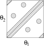
Figure 18: Neighborhood of the subset ${\mathcal{U}}$ for sufficiently small ${\mathsf{r}}_{\Lambda}>0$.

In writing $B_{b}({\mathsf{h}})$ for the open ball in $T^{2}$, we abuse notation somewhat. By assumption, the radius of $B_{b}({\mathsf{h}})$ is fixed so that this ball lies in the preimage of the corresponding disc ${D_{a}({\mathsf{h}})\subset{\mathbb{R}}^{2}}$ under the map ${\gamma^{-}_{a}\times\gamma^{+}_{a}}$ in Figure 15,

$$\left(\gamma^{-}_{a}\times\gamma^{+}_{a}\right)\!\left(B_{b}({\mathsf{h}})\right)\,\subset\,D_{a}({\mathsf{h}})\,,\qquad\qquad a\equiv b\mod n\,.$$ (159)

Therefore the radius of $B_{b}({\mathsf{h}})$ is not necessarily equal to ${\mathsf{h}}$, but it is determined by ${\mathsf{h}}$ independently of $\Lambda$. Once ${\mathsf{h}}$ is fixed in terms of the geometry of $C$, we can always take $\Lambda$ sufficiently large and ${{\mathsf{r}}_{\Lambda}\sim\Lambda^{-1/4}}$ sufficiently small so that $B_{b}({\mathsf{h}})$ contains the relevant portion of ${\mathcal{U}}$.

Similarly, the tubular neighborhood $N_{\Delta}({\mathsf{w}})$ of the diagonal has width ${{\mathsf{w}}>0}$, meaning that points in $N_{\Delta}({\mathsf{w}})$ satisfy ${|\theta_{2}-\theta_{1}|<{\mathsf{w}}}$ for the parameters in Figure 18. A crucial step will be to fix the value of ${\mathsf{w}}$, which must be large enough so that $N_{\Delta}({\mathsf{w}})$ contains the piece of ${\mathcal{U}}$ near the diagonal, but also small enough so that the local analysis from Section II.1 is applicable everywhere in $N_{\Delta}({\mathsf{w}})$.

According to the next lemma, both conditions on $N_{\Delta}({\mathsf{w}})$ can be simultaneously satisfied once we set

$${\mathsf{w}}\,=\,\frac{{\mathsf{r}}_{\Lambda}\sqrt{2}}{m}\,,$$ (160)

with a positive constant ${m>0}$ defined geometrically by

$$m^{2}\,=\,\min_{\theta\in S^{1}}\Big{[}||\dot{\gamma}(\theta)||^{2}\Big{]}\,.$$ (161)

Since ${\gamma=\Pi\circ X}$ is an immersion, the minimum speed in (161) is bounded away from zero, which is essential. The constant $\sqrt{2}$ is inessential and could be absorbed into the definition of $m$.

Lemma III.2

For sufficiently large $\Lambda$ and ${{\mathsf{w}}={\mathsf{r}}_{\Lambda}\sqrt{2}/m}$, the tubular neighborhood $N_{\Delta}({\mathsf{w}})$ contains the diagonal component of ${\mathcal{U}}$.

Proof The lemma says that, away from crossings, all points on the projection $\Pi(C)$ which lie within the distance ${\mathsf{r}}_{\Lambda}$ of a given point $\gamma(\theta)$ are contained within the image of the interval $\left[\theta-{\mathsf{r}}_{\Lambda}\sqrt{2}/m,\,\theta+{\mathsf{r}}_{\Lambda}\sqrt{2}/m\right]$ under $\gamma$, for all values of $\theta$. See Figure 19 for an illustration of this claim. The minimum speed along $\gamma$ naturally sets the scale of the required interval, which decreases with increasing $m$.

Figure 19: Points within the distance ${\mathsf{r}}_{\Lambda}$ of $\gamma(\theta)$.

For any fixed ${\theta_{0}\in S^{1}}$, define the function

$$F(\theta)=\frac{d}{d\theta}\big{|}\big{|}\gamma(\theta)-\gamma(\theta_{0})\big{|}\big{|}^{2}\,=\,2\,\big{(}\gamma(\theta)-\gamma(\theta_{0})\big{)}\cdot\dot{\gamma}(\theta)\,.$$ (162)

Then ${F(\theta_{0})=0}$, and the derivative of $F$ is

$$\frac{dF}{d\theta}(\theta)\,=\,2\,||\dot{\gamma}||^{2}\,+\,2\,\big{(}\gamma(\theta)-\gamma(\theta_{0})\big{)}\cdot\ddot{\gamma}(\theta)\,.$$ (163)

Since $\gamma$ is an immersion, ${||\dot{\gamma}||\geq m}$ is bounded below, and ${||\ddot{\gamma}||<\infty}$ is bounded above. So if ${||\gamma(\theta)-\gamma(\theta_{0})||\leq{\mathsf{r}}_{\Lambda}}$ for sufficiently large $\Lambda$ and hence sufficiently small ${\mathsf{r}}_{\Lambda}$, then

$$\frac{dF}{d\theta}(\theta)>m^{2}\,.$$ (164)

Integrating the inequality in (164), we obtain

$$F(\theta)\,>\,m^{2}\left|\theta-\theta_{0}\right|.$$ (165)

Integrating once more from the definition (162) of $F(\theta)$,

$$\big{|}\big{|}\gamma(\theta)-\gamma(\theta_{0})\big{|}\big{|}^{2}\,>\,\frac{1}{2}m^{2}\,|\theta-\theta_{0}|^{2}\,,$$ (166)

or

$$\big{|}\big{|}\gamma(\theta)-\gamma(\theta_{0})\big{|}\big{|}\,>\,\frac{m}{\sqrt{2}}\,|\theta-\theta_{0}|\,.$$ (167)

Thus if ${||\gamma(\theta)-\gamma(\theta_{0})||={\mathsf{r}}_{\Lambda}}$, then ${|\theta-\theta_{0}|<{\mathsf{r}}_{\Lambda}\sqrt{2}/m}$, which is the required bound.  $\square$

Because ${\mathcal{U}}$ is contained in the union of $N_{\Delta}({\mathsf{w}})$ and ${\cup B_{b}({\mathsf{h}})}$, we have a relation between the corresponding self-linking integrals,

$$\left|\int_{\mathcal{U}}\left(X\times X\right)^{*}\!\widehat{\Gamma}_{\hbar}^{*}\,\chi_{\Lambda}\,-\,\int_{N_{\Delta}({\mathsf{w}})}\mskip-25.0mu\left(X\times X\right)^{*}\!\widehat{\Gamma}_{\hbar}^{*}\,\chi_{\Lambda}\,-\,\sum_{b=1}^{2n}\int_{B_{b}({\mathsf{h}})}\mskip-25.0mu\left(X\times X\right)^{*}\!\widehat{\Gamma}_{\hbar}^{*}\,\chi_{\Lambda}\right|\,<\,M\,\delta\,.$$ (168)

This inequality again follows from Lemma III.1, because points contained in either $N_{\Delta}({\mathsf{w}})$ or $B_{b}({\mathsf{h}})$ but not in ${\mathcal{U}}$ lie in ${\mathcal{V}}$, where the magnitude of the self-linking integrand is bounded by $\delta$. So for sufficiently large $\Lambda$, we just need to evaluate the self-linking integral over the balls $B_{b}({\mathsf{h}})$ and the tubular neighborhood $N_{\Delta}({\mathsf{w}})$ in Figure 18.

Error analysis at a crossing

We first evaluate the self-linking integral over the ball $B_{b}({\mathsf{h}})$. By the positivity condition on the heat form $\chi_{\Lambda}$, the self-linking integrand vanishes in exactly half the balls. Reshuffling indices as necessary, we consider only those $B_{a}({\mathsf{h}})$ for ${a=1,\ldots,n}$ on which ${\widehat{\Delta}z>0}$ and the integrand is non-zero.

With malice aforethought, we have arranged that the image of $B_{a}({\mathsf{h}})$ under the product map ${\gamma^{-}_{a}\times\gamma^{+}_{a}}$ lies in the disc ${D_{a}({\mathsf{h}})\subset{\mathbb{R}}^{2}}$, where we have control over the geometry of $C$. In particular, the map $\varphi_{a}$ in Figure 16 restricts to a diffeomorphism from $B_{a}({\mathsf{h}})$ to a curvy quadrilateral region ${\mathcal{Q}}$ about the origin in the $uv$-plane,

$$\varphi_{a}\,=\,\gamma^{+}_{a}(\theta_{2})-\gamma^{-}_{a}(\theta_{1})\,\equiv\,\left(u(\theta_{1},\theta_{2}),v(\theta_{1},\theta_{2})\right)\,.$$ (169)

Our analysis will be performed using the $uv$-coordinates. In these coordinates, the self-linking integrand (108) simplifies,

$$\frac{\Lambda}{2\pi\widehat{\Delta}z}\,{\rm e}^{\,\!-\Lambda(\Delta x^{2}+\Delta y^{2})/2\widehat{\Delta}z}\left[d\Delta x{\wedge}d\Delta y\,+\frac{1}{2}\left(\Delta x\,d\Delta y-\Delta y\,d\Delta x\right)\!{\wedge}\frac{d\widehat{\Delta}z}{\widehat{\Delta}z}\right]$$ (170)

$$\qquad\,=\,\frac{\Lambda}{2\pi\widehat{\Delta}z(u,v)}\,{\rm e}^{\,\!-\Lambda(u^{2}+v^{2})/2\widehat{\Delta}z(u,v)}\left[du{\wedge}dv\,+\frac{1}{2}\left(u\,dv-v\,du\right)\!{\wedge}\frac{d\widehat{\Delta}z(u,v)}{\widehat{\Delta}z(u,v)}\right].$$

Here $\Delta x$ and $\Delta y$ are identified with the Cartesian coordinates $u$ and $v$, and $\widehat{\Delta}z$ is considered to be a function of $(u,v)$. All unknown functional dependence of the self-linking integrand in (170) is absorbed into ${\widehat{\Delta}z(u,v)}$.

The integrand in (170) is a sum of two terms,

$$\Psi\,=\,\frac{\Lambda}{2\pi\widehat{\Delta}z(u,v)}\,{\rm e}^{\,\!-\Lambda(u^{2}+v^{2})/2\widehat{\Delta}z(u,v)}\,du{\wedge}dv\,,$$ (171)

and

$$\Xi\,=\,\frac{\Lambda}{4\pi\widehat{\Delta}z(u,v)}\,{\rm e}^{\,\!-\Lambda(u^{2}+v^{2})/2\widehat{\Delta}z(u,v)}\left(u\,dv-v\,du\right)\!{\wedge}\frac{d\widehat{\Delta}z(u,v)}{\widehat{\Delta}z(u,v)}\,.$$ (172)

Hence after making the change-of-variables in ${\mathcal{Q}}$,

$$\int_{B_{a}({\mathsf{h}})}\left(X\times X\right)^{*}\!\widehat{\Gamma}_{\hbar}^{*}\,\chi_{\Lambda}\,=\,\int_{\mathcal{Q}}\Psi\,+\,\int_{\mathcal{Q}}\Xi\,.$$ (173)

The analysis of the two terms on the right in (173) is different. Morally, $\Xi$ is higher-order in $u$ and $v$ so will be irrelevant when $\Lambda$ is large and ${u,v\ll 1/\Lambda}$. By contrast, $\Psi$ is always relevant. We analyze the integrals of $\Psi$ and $\Xi$ over ${\mathcal{Q}}$ in turn.

$$\begin{matrix}&\begin{picture}(1.0,0.92238)\put(0.0,0.0){\includegraphics[width=128.0374pt]{107+.eps}}\put(0.63442,0.75){\color[rgb]{0,0,0}\makebox(0.0,0.0)[lb]{\smash{$\gamma^{+}$}}}\put(0.6,0.42){\color[rgb]{0,0,0}\makebox(0.0,0.0)[lb]{\smash{$\gamma^{-}$}}}\end{picture}\qquad&\qquad&\begin{picture}(1.0,0.92238)\put(0.0,0.0){\includegraphics[width=128.0374pt]{107-.eps}}\put(0.63442,0.75){\color[rgb]{0,0,0}\makebox(0.0,0.0)[lb]{\smash{$\gamma^{+}$}}}\put(0.6,0.42){\color[rgb]{0,0,0}\makebox(0.0,0.0)[lb]{\smash{$\gamma^{-}$}}}\end{picture}\\ &(a.)\quad\deg(\varphi_{a})=+1\qquad&\qquad&(b.)\quad\deg(\varphi_{a})=-1\end{matrix}$$

Figure 20: Sign of the Jacobian for $\varphi_{a}$.

Integral of $\Psi$

Explicitly, the integral of $\Psi$ is given by a kind of nonlinear Gaussian,

$$\int_{\mathcal{Q}}\Psi\,=\,\deg(\varphi_{a})\int_{\mathcal{Q}}\frac{\Lambda}{2\pi\widehat{\Delta}z(u,v)}\,\exp{\!\left[-\frac{\Lambda\left(u^{2}+v^{2}\right)}{2\,\widehat{\Delta}z(u,v)}\right]}\,du\,dv\,,\qquad\widehat{\Delta}z(u,v)>0\,.$$ (174)

Here ${\deg(\varphi_{a})=\pm 1}$ depending upon whether the diffeomorphism ${\varphi_{a}:B_{a}({\mathsf{h}})\to{\mathcal{Q}}}$ preserves or reverses orientation. Equivalently, from the expression in (169), the sign is determined by the Jacobian in the expansion

$$du{\wedge}dv\,=\,-\left(\frac{d\gamma^{-}}{d\theta_{1}}\times\frac{d\gamma^{+}}{d\theta_{2}}\right)d\theta_{1}{\wedge}d\theta_{2}\,.$$ (175)

By inspection of Figure 20, $\deg(\varphi_{a})$ is exactly the local writhe at the given crossing,

$$\deg(\varphi_{a})\,=\,{\mathsf{w}}_{a}\,.$$ (176)

To suppress pernicious signs for the remainder, we assume ${{\mathsf{w}}_{a}=+1}$.

For large $\Lambda$, we evaluate the integral of $\Psi$ over ${\mathcal{Q}}$ in two steps.

• We replace the unknown function $\widehat{\Delta}z(u,v)$ by the constant displacement $\Delta z_{a}$ at the crossing, with error

  $$\left|\int_{\mathcal{Q}}\frac{\Lambda}{2\pi\widehat{\Delta}z(u,v)}\exp{\left[-\frac{\Lambda\left(u^{2}+v^{2}\right)}{2\,\widehat{\Delta}z(u,v)}\right]}du\,dv\,-\,\int_{\mathcal{Q}}\frac{\Lambda}{2\pi\Delta z_{a}}\exp{\!\left[-\frac{\Lambda\left(u^{2}+v^{2}\right)}{2\,\Delta z_{a}}\right]}du\,dv\right|<\,M\delta\,.$$ (177)

• We extend the subsequent range of Gaussian integration from ${\mathcal{Q}}$ to ${\mathbb{R}}^{2}$ so that the Gaussian integral can be performed analytically, with error

  $$\left|\int_{\mathcal{Q}}\frac{\Lambda}{2\pi\Delta z_{a}}\exp{\!\left[-\frac{\Lambda\left(u^{2}+v^{2}\right)}{2\,\Delta z_{a}}\right]}du\,dv-\int_{{\mathbb{R}}^{2}}\frac{\Lambda}{2\pi\Delta z_{a}}\exp{\!\left[-\frac{\Lambda\left(u^{2}+v^{2}\right)}{2\,\Delta z_{a}}\right]}du\,dv\right|<\,\delta\,.$$ (178)

Of these steps, only the first is non-trivial. For the second, because the Gaussian integral over ${\mathbb{R}}^{2}$ is normalized to unity independent of $\Lambda$, we can always choose $\Lambda$ sufficiently large so that

$$\int_{{\mathbb{R}}^{2}-{\mathcal{Q}}}\frac{\Lambda}{2\pi\Delta z_{a}}\exp{\!\left[-\frac{\Lambda\left(u^{2}+v^{2}\right)}{2\,\Delta z_{a}}\right]}du\,dv\,<\,\delta\,.$$ (179)

Informally, we performed both these steps in arriving at (118).

For the first step, we use heavily the positive function ${\mathsf{R}}_{a}(\Lambda)$ which satisfies

$$\frac{\Lambda}{2\pi\Delta z_{a}}\exp{\!\left[-\frac{\Lambda\,{\mathsf{R}}_{a}(\Lambda)^{2}}{2\Delta z_{a}}\right]}\,=\,\delta\,,$$ (180)

and vanishes monotonically as ${\Lambda\to\infty}$. The function ${\mathsf{R}}_{a}(\Lambda)$ sets the minimum distance from the origin for which the Gaussian integrand in (177) becomes negligible.

To be on the safe side in our bounds, we will have to work with a slightly larger distance ${{\mathsf{R}}_{a}(\Lambda/2)>{\mathsf{R}}_{a}(\Lambda)}$. Let ${B_{0}\equiv B_{0}({\mathsf{R}}_{a}(\Lambda/2))}$ be the ball of radius ${\mathsf{R}}_{a}(\Lambda/2)$ which is centered at the origin in ${\mathcal{Q}}$,

$$B_{0}:\quad u^{2}+v^{2}\,<\,{\mathsf{R}}_{a}^{2}(\Lambda/2)\,.$$ (181)

We shall prove that when $(u,v)$ lies in $B_{0}$, the difference between the nonlinear and the usual Gaussian in (177) is small,

$$\left|\int_{B_{0}}\frac{\Lambda}{2\pi\widehat{\Delta}z(u,v)}\exp{\!\left[-\frac{\Lambda\left(u^{2}+v^{2}\right)}{2\widehat{\Delta}z(u,v)}\right]}du\,dv\,-\,\int_{B_{0}}\frac{\Lambda}{2\pi\Delta z_{a}}\exp{\!\left[-\frac{\Lambda\left(u^{2}+v^{2}\right)}{2\Delta z_{a}}\right]}du\,dv\right|\,<\,\delta\,.$$ (182)

Otherwise, when $(u,v)$ lies outside $B_{0}$ in ${\mathcal{Q}}$, we show that both integrals are separately small, with

$$\int_{{\mathcal{Q}}-B_{0}}\frac{\Lambda}{2\pi\widehat{\Delta}z(u,v)}\exp{\!\left[-\frac{\Lambda\left(u^{2}+v^{2}\right)}{2\widehat{\Delta}z(u,v)}\right]}du\,dv\,<M\,\delta\,,$$ (183)

and

$$\int_{{\mathcal{Q}}-B_{0}}\frac{\Lambda}{2\pi\Delta z_{a}}\exp{\!\left[-\frac{\Lambda\left(u^{2}+v^{2}\right)}{2\Delta z_{a}}\right]}du\,dv\,<\,M\,\delta\,.$$ (184)

Thus the difference must also be small in ${{\mathcal{Q}}-B_{0}}$. This trick is the engine of asymptotic analysis. See Ch. $6$ in Bender:1999 for further background on this idea.

We begin by establishing some easy bounds when $(u,v)$ lies inside the ball ${B_{0}\subset{\mathcal{Q}}}$. From the definition of ${\mathsf{R}}_{a}(\Lambda/2)$,

$$u^{2}+v^{2}<{\mathsf{R}}_{a}^{2}(\Lambda/2)\,=\,\frac{4\Delta z_{a}}{\Lambda}\ln\frac{\Lambda}{4\pi\Delta z_{a}\delta}\,,$$ (185)

so the argument of the Gaussian is bounded by

$$\frac{\Lambda(u^{2}+v^{2})}{2\Delta z_{a}}<2\ln\frac{\Lambda}{4\pi\Delta z_{a}\delta}\,.$$ (186)

On the other hand, consider the difference ${\widehat{\Delta}z(u,v)-\Delta z_{a}}$. As a function of $(u,v)$, the difference vanishes at ${u=v=0}$ and is differentiable there, so

$$\big{|}\widehat{\Delta}z(u,v)-\Delta z_{a}\big{|}\,<\,M\sqrt{u^{2}+v^{2}}\,<\,M\,{\mathsf{R}}_{a}(\Lambda/2)\,,$$ (187)

for some constant $M$ depending on $C$. Immediately, since ${\mathsf{R}}_{a}^{2}(\Lambda/2)$ scales like ${\ln\Lambda/\Lambda}$, the relative fluctuations in height about $\Delta z_{a}$ satisfy

$$\frac{\big{|}\widehat{\Delta}z(u,v)-\Delta z_{a}\big{|}}{\Delta z_{a}}\,<\,\frac{M\,{\mathsf{R}}_{a}(\Lambda/2)}{\Delta z_{a}}\,\sim\,\left(\frac{\ln\Lambda}{\Lambda}\right)^{1/2}\,.$$ (188)

Directly from (186) and (188),

$$\frac{\Lambda(u^{2}+v^{2})}{2\,\Delta z_{a}}\cdot\frac{\big{|}\widehat{\Delta}z(u,v)-\Delta z_{a}\big{|}}{\Delta z_{a}}\,<\,M\,\frac{(\ln\Lambda)^{3/2}}{\Lambda^{1/2}}\,.$$ (189)

The constant $M$ in (189) is not necessarily the same as the constant $M$ in (188)!

Given the relative similarity between the integrands in (182), we consider their ratio

$$q\,=\,\frac{\Lambda}{2\pi\widehat{\Delta}z(u,v)}\exp{\!\left[-\frac{\Lambda\left(u^{2}+v^{2}\right)}{2\widehat{\Delta}z(u,v)}\right]}\Biggr{/}\frac{\Lambda}{2\pi\Delta z_{a}}\exp{\!\left[-\frac{\Lambda\left(u^{2}+v^{2}\right)}{2\Delta z_{a}}\right]}\,.$$ (190)

With some algebra, this ratio can be recast as

$$q =\,\frac{\Delta z_{a}}{\widehat{\Delta}z(u,v)}\exp{\!\left[\frac{\Lambda\left(u^{2}+v^{2}\right)}{2}\cdot\frac{\widehat{\Delta}z(u,v)-\Delta z_{a}}{\widehat{\Delta}z(u,v)\Delta z_{a}}\right]}\,,$$ (191)

$$=\left[1\,+\,\frac{\widehat{\Delta}z(u,v)-\Delta z_{a}}{\Delta z_{a}}\right]^{-1}\cdot\exp{\!\left[\frac{\Lambda\left(u^{2}+v^{2}\right)}{2\Delta z_{a}}\cdot\frac{\widehat{\Delta}z(u,v)-\Delta z_{a}}{\Delta z_{a}}\cdot\frac{\Delta z_{a}}{\widehat{\Delta}z(u,v)}\right]}\,.$$

By the estimates in (188) and (189), the prefactor in $q$ approaches unity and the argument of the exponential vanishes as ${\Lambda\to\infty}$. Hence we can choose $\Lambda$ sufficiently large so that

$$|q-1|\,<\,\delta\,.$$ (192)

With this control over the fractional error, the difference between the nonlinear and the usual Gaussian in (182) is bounded by

$$\int_{B_{0}}\left|\frac{\Lambda}{2\pi\widehat{\Delta}z(u,v)}\exp{\!\left[-\frac{\Lambda\left(u^{2}+v^{2}\right)}{2\widehat{\Delta}z(u,v)}\right]}\,-\,\frac{\Lambda}{2\pi\Delta z_{a}}\exp{\!\left[-\frac{\Lambda\left(u^{2}+v^{2}\right)}{2\Delta z_{a}}\right]}\right|du\,dv$$ (193)

$$\qquad\qquad\leq\int_{B_{0}}\frac{\Lambda\,|q-1|}{2\pi\Delta z_{a}}\exp{\!\left[-\frac{\Lambda\left(u^{2}+v^{2}\right)}{2\Delta z_{a}}\right]}du\,dv$$

$$\qquad\qquad<\,\int_{B_{0}}\frac{\Lambda\,\delta}{2\pi\Delta z_{a}}\exp{\!\left[-\frac{\Lambda\left(u^{2}+v^{2}\right)}{2\Delta z_{a}}\right]}du\,dv\,<\,\delta\,.$$

We are left to examine what happens when $(u,v)$ lies outside the ball ${B_{0}\subset{\mathcal{Q}}}$ of radius ${{\mathsf{R}}_{a}(\Lambda/2)}$, meaning

$$u^{2}+v^{2}\geq{\mathsf{R}}_{a}^{2}(\Lambda/2)\,.$$ (194)

To start, the bound on the Gaussian in (184) is trivial because the integrand is bounded by $\delta$ for all points $(u,v)$ outside the ball of radius ${\mathsf{R}}_{a}(\Lambda)$, and ${{\mathsf{R}}_{a}(\Lambda/2)>{\mathsf{R}}_{a}(\Lambda)}$. So the real task is to establish the bound for the nonlinear Gaussian in (183).

Consider the following function on ${\mathcal{Q}}$,

$$\widehat{\Lambda}(u,v)\,=\,\Lambda\cdot\frac{\Delta z_{a}}{\widehat{\Delta}z(u,v)}\,.$$ (195)

Conceptually, we interpret $\widehat{\Lambda}$ as a fluctuating, position-dependent version of the parameter $\Lambda$, so that the width of the nonlinear Gaussian varies from point-to-point on ${\mathcal{Q}}$. By the estimate in (138), the relative fluctuation factor is bounded from below everywhere on ${\mathcal{Q}}$ by

$$\frac{1}{2}\,<\,1\,-\,{\mathsf{c}}\,<\,\frac{\Delta z_{a}}{\widehat{\Delta}z(u,v)}\,.$$ (196)

Consequently, by the definition of $\widehat{\Lambda}$,

$$\frac{\Lambda}{2}\,<\,\widehat{\Lambda}(u,v)\,.$$ (197)

Associated to the local parameter $\widehat{\Lambda}(u,v)$ we have a local scale ${\mathsf{R}}_{a}(\widehat{\Lambda}(u,v))$, also a function of $u$ and $v$. Since ${\mathsf{R}}_{a}$ is monotonically decreasing for large $\Lambda$, the lower bound on $\widehat{\Lambda}$ in (197) means that

$${\mathsf{R}}_{a}^{2}(\widehat{\Lambda}(u,v))\,<\,{\mathsf{R}}_{a}^{2}(\Lambda/2)\,<\,u^{2}+v^{2}\,.$$ (198)

Thus, again by the definition of ${\mathsf{R}}_{a}(\Lambda)$ in (180),

$$\frac{\widehat{\Lambda}}{2\pi\Delta z_{a}}\exp{\!\left[-\frac{\widehat{\Lambda}\left(u^{2}+v^{2}\right)}{2\,\Delta z_{a}}\right]}\,<\,\delta\,,$$ (199)

or by substitution from (195),

$$\frac{\Lambda}{2\pi\widehat{\Delta}z(u,v)}\exp{\!\left[-\frac{\Lambda\left(u^{2}+v^{2}\right)}{2\,\widehat{\Delta}z(u,v)}\right]}\,<\,\delta\,.$$ (200)

The bound on the nonlinear Gaussian in (200) is exactly what we need to control the integral over ${{\mathcal{Q}}-B_{0}}$, so that

$$\int_{{\mathcal{Q}}-B_{0}}\frac{\Lambda}{2\pi\widehat{\Delta}z(u,v)}\exp{\!\left[-\frac{\Lambda\left(u^{2}+v^{2}\right)}{2\widehat{\Delta}z(u,v)}\right]}du\,dv\,<\,M\,\delta\,.$$ (201)

Combining with the trivial bound in (178), we deduce that the desired integral of $\Psi$ over ${\mathcal{Q}}$ can be well-approximated for large $\Lambda$ by the naive Gaussian integral,

$$\left|\int_{\mathcal{Q}}\Psi\,-\,\deg(\varphi_{a})\int_{{\mathbb{R}}^{2}}\frac{\Lambda}{2\pi\Delta z_{a}}\exp{\!\left[-\frac{\Lambda\left(u^{2}+v^{2}\right)}{2\Delta z_{a}}\right]}du\,dv\right|<\,M\,\delta\,.$$ (202)

Integral of $\Xi$

We are not finished with our error analysis at the crossing, because we still must consider the integral of $\Xi$ over ${\mathcal{Q}}$ in (173). We will show that the contribution of $\Xi$ is negligible for large $\Lambda$,

$$\left|\int_{\mathcal{Q}}\Xi\,\right|\,<\,M\,\delta\,.$$ (203)

Explicitly, from the formula in (172), the integral of $\Xi$ is given in the $(u,v)$-coordinates by

$$\int_{\mathcal{Q}}\Xi\,=\,-\int_{\mathcal{Q}}\frac{\Lambda}{4\pi\widehat{\Delta}z(u,v)^{2}}\,{\rm e}^{\,\!-\Lambda(u^{2}+v^{2})/2\widehat{\Delta}z(u,v)}\left(u\frac{\partial\widehat{\Delta}z}{\partial u}\,+\,v\frac{\partial\widehat{\Delta}z}{\partial v}\right)du\,dv\,.$$ (204)

Again, we consider the cases that $(u,v)$ lies inside the ball $B_{0}$ and outside the ball $B_{0}$ separately. When $(u,v)$ lies outside the ball ${B_{0}\subset{\mathcal{Q}}}$, then by the definition of ${\mathsf{R}}_{a}(\Lambda)$ in (180),

$$\left|\frac{\Lambda}{4\pi\widehat{\Delta}z(u,v)^{2}}\,{\rm e}^{\,\!-\Lambda(u^{2}+v^{2})/2\widehat{\Delta}z(u,v)}\left(u\frac{\partial\widehat{\Delta}z}{\partial u}\,+\,v\frac{\partial\widehat{\Delta}z}{\partial v}\right)\right|<\,M\,\delta\,.$$ (205)

Here we note that the extra factors of ${1/\widehat{\Delta}z}$ and ${\left(u\,\partial/\partial u+v\,\partial/\partial v\right)\widehat{\Delta}z}$ in (205) are smooth functions bounded independently of $\Lambda$ on ${\mathcal{Q}}$. These functions do not alter the bound by $\delta$ but are absorbed into the constant $M$.

Otherwise, for points inside $B_{0}$, we have a bound

$$\int_{B_{0}}\frac{\Lambda}{4\pi\widehat{\Delta}z(u,v)^{2}}\exp{\!\left[-\frac{\Lambda\left(u^{2}+v^{2}\right)}{2\widehat{\Delta}z(u,v)}\right]}du\,dv\,<M\,,$$ (206)

which follows by the same arguments used to produce the estimate in (193). Also, since ${\left(u\,\partial/\partial u+v\,\partial/\partial v\right)\widehat{\Delta}z}$ is bounded in $B_{0}$ and ${|u|,|v|\leq{\mathsf{R}}_{a}(\Lambda/2)\to 0}$ as $\Lambda\to\infty$, we can always choose $\Lambda$ so that

$$\left|u\frac{\partial\widehat{\Delta}z}{\partial u}\,+\,v\frac{\partial\widehat{\Delta}z}{\partial v}\right|<\,\delta\,,$$ (207)

for all $(u,v)$ in $B_{0}$. Combining the bounds in (205), (206), and (207) for outside and inside $B_{0}$, we obtain the conclusion in (203).

In summary, these bounds establish the informal localization formula in (119) for any crossing of $\Pi(C)$.  $\square$

Error analysis near the diagonal

Our final goal is to evaluate the self-linking integral over the tubular neighborhood $N_{\Delta}({\mathsf{w}})$ of the diagonal ${\Delta\subset T^{2}}$, where ${{\mathsf{w}}\sim\Lambda^{-1/4}}$ is the width set in Lemma III.2. For the informal localization computation in (120), we used the leading term in the Taylor expansion of the self-linking integrand near the diagonal to approximate the integral. Depending upon the value of the parameter $\hbar$, we abbreviate this leading term by

$$\Phi_{\hbar}\,\buildrel\hbar\neq 1\over{=}\,-\operatorname{\mathrm{sgn}}(\eta)\,\frac{\Lambda\left(\dot{\gamma}\times\ddot{\gamma}\right)}{4\pi\,|1-\hbar|\,|\gamma\times\dot{\gamma}|}\,\exp{\!\left[-\frac{\Lambda\,||\dot{\gamma}||^{2}\,|\eta|}{2\,|1-\hbar|\,|\gamma\times\dot{\gamma}|}\right]}\,d\phi{\wedge}d\eta\,,$$ (208)

or

$$\Phi_{\hbar}\,\buildrel\hbar=1\over{=}\,-\frac{3\,\Lambda}{2\pi\eta^{2}}\exp{\!\left[-\frac{3\,\Lambda\,||\dot{\gamma}||^{2}}{\left|\dot{\gamma}\times\ddot{\gamma}\right|}\frac{1}{|\eta|}\right]}\,d\phi{\wedge}d\eta\,.$$ (209)

In both cases we assume that the local positivity condition ${\widehat{\Delta}z>0}$ is satisfied, as in (76). Otherwise, ${\Phi_{\hbar}\equiv 0}$.

To justify our localization computation, we must demonstrate for sufficiently large $\Lambda$ the bound

$$\left|\int_{N_{\Delta}({\mathsf{w}})}\mskip-25.0mu\left(X\times X\right)^{*}\!\widehat{\Gamma}_{\hbar}^{*}\,\chi_{\Lambda}\,-\,\int_{N_{\Delta}({\mathsf{w}})}\mskip-15.0mu\Phi_{\hbar}\,\right|<M\,\delta\,.$$ (210)

The behavior of $\Phi_{\hbar}$ for small $\eta$ depends very much on whether $\hbar$ is equal to one or not, so we treat the cases in (208) and (209) separately. Because the generic case ${\hbar\neq 1}$ is the more involved, and the more interesting, we begin with it.

Generic case ${\hbar\neq 1}$

In principle, the error in the leading approximation to $\left(X\times X\right)^{*}\!\widehat{\Gamma}_{\hbar}^{*}\,\chi_{\Lambda}$ for small $\eta$ is controlled by the magnitude of the next-order term in the Taylor expansion. We will need this correction term for our analysis. Briefly, by the same computations leading to (75) in Section II.1, the argument of the heat kernel admits the second-order expansion

$$\frac{\Delta x^{2}+\Delta y^{2}}{2\,\widehat{\Delta}z}\,\buildrel\hbar\neq 1\over{=}\,-\frac{||\dot{\gamma}||^{2}\,\eta}{2\left(1-\hbar\right)\left(\gamma\times\dot{\gamma}\right)}\left[1\,+\left(\frac{\dot{\gamma}\cdot\ddot{\gamma}}{||\dot{\gamma}||^{2}}-\frac{1}{2}\frac{\gamma\times\ddot{\gamma}}{\gamma\times\dot{\gamma}}\right)\eta\,+\,{\mathcal{O}}\big{(}\eta^{2}\big{)}\right],$$ (211)

where ${\dot{\gamma}\cdot\ddot{\gamma}\equiv\dot{x}\,\ddot{x}+\dot{y}\,\ddot{y}}$. Similarly for the pullback of the heat form $\chi_{\Lambda}$ itself,

$$\left(X\times X\right)^{*}\!\widehat{\Gamma}_{\hbar}^{*}\,\chi_{\Lambda}\,\buildrel\hbar\neq 1\over{=}\,$$ (212)

$$-\frac{\Lambda\,\operatorname{\mathrm{sgn}}(\eta)\,d\phi{\wedge}d\eta}{4\pi\,|1-\hbar|\,|\gamma\times\dot{\gamma}|}\left[\left(\dot{\gamma}\times\ddot{\gamma}\right)\,+\,\left(\frac{1}{2}\left(\dot{\gamma}\times\dddot{\gamma}\right)-\frac{\left(\gamma\times\ddot{\gamma}\right)\left(\dot{\gamma}\times\ddot{\gamma}\right)}{\left(\gamma\times\dot{\gamma}\right)}\right)\eta\,+\,{\mathcal{O}}\big{(}\eta^{2}\big{)}\right]\times$$

$$\times\,\exp{\!\left[-\frac{\Lambda\,||\dot{\gamma}||^{2}\,|\eta|}{2\left|1-\hbar\right|\left|\gamma\times\dot{\gamma}\right|}\left(1\,+\left(\frac{\dot{\gamma}\cdot\ddot{\gamma}}{||\dot{\gamma}||^{2}}-\frac{1}{2}\frac{\gamma\times\ddot{\gamma}}{\gamma\times\dot{\gamma}}\right)\eta\,+\,{\mathcal{O}}\big{(}\eta^{2}\big{)}\right)\right]}\,.$$

We omit the computation leading to (212), since the details of this formula will not be so important. The expansion merely confirms that both the prefactor and the argument of the exponential for $\Phi_{\hbar}$ in (208) receive further corrections at the next order in $\eta$, as determined by the geometry of the projection $\Pi(C)$.

Validity of the leading approximation $\Phi_{\hbar}$ requires that the correction terms in (212) be small. At least informally, for the argument of the heat kernel in (211) we require

$$\left|\,\left(\frac{\dot{\gamma}\cdot\ddot{\gamma}}{||\dot{\gamma}||^{2}}-\frac{1}{2}\frac{\gamma\times\ddot{\gamma}}{\gamma\times\dot{\gamma}}\right)\eta\,\right|\ll 1\,.$$ (213)

By assumption, ${|\eta|<{\mathsf{w}}\sim\Lambda^{-1/4}}$ is always small on $N_{\Delta}({\mathsf{w}})$, and ${||\dot{\gamma}||^{2}>0}$ is bounded from below. The condition in (213) is therefore only violated at points where ${\gamma\times\dot{\gamma}=0}$. At these points, the Taylor expansion in (212) breaks down.

Despite the failure of the Taylor expansion at points where ${\gamma\times\dot{\gamma}=0}$, these points cause no difficulty. Recall that points where ${\gamma\times\dot{\gamma}=0}$ correspond to critical points of the height function $z(\theta)$ on $C$. By the Morse assumption which follows Lemma II.1, the function ${\left(\gamma\times\dot{\gamma}\right)(\phi)}$ vanishes at only a finite number of isolated critical points $\{\phi_{1},\ldots,\phi_{2k}\}$ on $S^{1}$. According to the analysis at the end of Section II.2, these points are precisely the endpoints of the disjoint collection of intervals ${S^{1}_{\pm}\cap\left[T^{2}-\Delta(\varepsilon)\right]}$ in (89). At the endpoints, $\Phi_{\hbar}$ vanishes, and the exact integrand $\left(X\times X\right)^{*}\!\widehat{\Gamma}_{\hbar}^{*}\,\chi_{\Lambda}$ in (108) is exponentially small (since $\widehat{\Delta}z$ is small). Consequently, the troublesome points for the Taylor expansion can just be removed from the domain of integration, with negligible error.

Figure 21: Domain $N_{\Delta}({\mathsf{w}};\ell)$ on which ${|\gamma\times\dot{\gamma}|>m>0}$.

Technically, about each critical point $\phi_{c}$,

$$\left(\gamma\times\dot{\gamma}\right)(\phi_{c})\,=\,0\,,\qquad\qquad c=1,\,\ldots,\,2k\,,$$ (214)

we consider a small neighborhood $(\phi_{c}-\ell,\phi_{c}+\ell)$ with fixed width ${\ell>0}$. Let ${\textrm{I}_{c}(\ell)\subset N_{\Delta}({\mathsf{w}})}$ be the corresponding closed strip

$$\textrm{I}_{c}(\ell)\,=\,\big{\{}(\phi,\eta)\,\big{|}\,|\phi-\phi_{c}|\leq\ell,\,|\eta|\leq{\mathsf{w}}\big{\}}\,,$$ (215)

and set

$$N_{\Delta}({\mathsf{w}};\ell)\,=\,N_{\Delta}({\mathsf{w}})\,-\,\bigcup_{c=1}^{2k}\,\textrm{I}_{c}(\ell)\,.$$ (216)

See Figure 21 for a sketch of $N_{\Delta}({\mathsf{w}};\ell)$ near one boundary of the cylinder ${T^{2}-\Delta(\varepsilon)}$. The shaded regions indicate the strips of width $\ell$ which have been excised about a pair of zeroes $\phi_{1}$ and $\phi_{2}$ of the function $\gamma\times\dot{\gamma}$.

We choose the width ${\ell>0}$ of each strip to be small enough so that

$$\left|\sum_{c=1}^{2k}\,\int_{\textrm{I}_{c}(\ell)}\left(X\times X\right)^{*}\!\widehat{\Gamma}_{\hbar}^{*}\,\chi_{\Lambda}\right|\,<\,\delta\,,\qquad\qquad\left|\sum_{c=1}^{2k}\,\int_{\textrm{I}_{c}(\ell)}\Phi_{\hbar}\,\right|\,<\,\delta\,.$$ (217)

Both integrands in (217) are bounded at the points $\phi_{c}$, so the integrals over $\textrm{I}_{c}(\ell)$ can be made as small as desired by the choice of $\ell$. Moreover, both integrands are decreasing functions of $\Lambda$ for sufficiently large $\Lambda$, so the width $\ell$ can be chosen independently of $\Lambda$, our crucial requirement.

By definition, the function $(\gamma\times\dot{\gamma})(\phi)$ is now bounded away from zero everywhere on the new domain $N_{\Delta}({\mathsf{w}};\ell)$,

$$\left|\gamma\times\dot{\gamma}\right|\,>\,m\,>\,0\quad\hbox{ on }\quad N_{\Delta}({\mathsf{w}};\ell)\,.$$ (218)

Here $m$ is a constant which depends upon the curve $C$ and the parameter ${\ell}$, but not on $\Lambda$. Because the respective contributions (217) from the excised strips are small by assumption, we are free to replace $N_{\Delta}({\mathsf{w}})$ by $N_{\Delta}({\mathsf{w}};\ell)$ in the inequality (210) to be proven. On the other hand, due to the lower bound in (218), we will also have uniform control of error terms such as (213) in the Taylor approximation on $N_{\Delta}({\mathsf{w}};\ell)$.

The remainder of the discussion proceeds in rough correspondence to the asymptotic analysis near a crossing. By analogy to the ball $B_{0}$ in (181), we introduce a smaller tubular neighborhood ${N_{0}\subset N_{\Delta}({\mathsf{w}};\ell)}$ defined by

$$N_{0}:\quad|\eta|\,<\,\frac{{\mathsf{w}}}{\sqrt{\Lambda}}\,\sim\,\Lambda^{-3/4}\,.$$ (219)

We indicate the coaxial configuration schematically in Figure 21. For points inside the small tube $N_{0}$, we will show that the difference between the integrals of $\left(X\times X\right)^{*}\!\widehat{\Gamma}_{\hbar}^{*}\,\chi_{\Lambda}$ and $\Phi_{\hbar}$ is small,

$$\left|\int_{N_{0}}\mskip-10.0mu\left(X\times X\right)^{*}\!\widehat{\Gamma}_{\hbar}^{*}\,\chi_{\Lambda}\,-\,\int_{N_{0}}\mskip-5.0mu\Phi_{\hbar}\,\right|<M\,\delta\,.$$ (220)

For points outside $N_{0}$ but inside $N_{\Delta}({\mathsf{w}};\ell)$, we will show that both integrals are separately small, with

$$\left|\int_{N_{\Delta}({\mathsf{w}};\ell)-N_{0}}\left(X\times X\right)^{*}\!\widehat{\Gamma}_{\hbar}^{*}\,\chi_{\Lambda}\,\right|\,<\,M\,\delta\,,$$ (221)

and

$$\left|\int_{N_{\Delta}({\mathsf{w}};\ell)-N_{0}}\Phi_{\hbar}\,\right|\,<\,M\,\delta\,.$$ (222)

The extra factor of $1/\sqrt{\Lambda}$ in the definition of $N_{0}$ is simply what is needed to ensure the inequality in (220).

We first consider the points inside $N_{0}$. From the second-order expansion in (212), the ratio of the self-linking integrand to its approximation $\Phi_{\hbar}$ satisfies

$$q\,=\,\frac{\left(X\times X\right)^{*}\!\widehat{\Gamma}_{\hbar}^{*}\,\chi_{\Lambda}}{\Phi_{\hbar}} =\,\left[1\,+\left(\frac{1}{2}\frac{\dot{\gamma}\times\dddot{\gamma}}{\dot{\gamma}\times\ddot{\gamma}}-\frac{\gamma\times\ddot{\gamma}}{\gamma\times\dot{\gamma}}\right)\eta\,+\,{\mathcal{O}}\big{(}\eta^{2}\big{)}\right]\times$$ (223)

$$\times\,\exp{\!\left[-\frac{\Lambda\,||\dot{\gamma}||^{2}\,|\eta|}{2\left|1-\hbar\right|\left|\gamma\times\dot{\gamma}\right|}\left(\frac{\dot{\gamma}\cdot\ddot{\gamma}}{||\dot{\gamma}||^{2}}-\frac{1}{2}\frac{\gamma\times\ddot{\gamma}}{\gamma\times\dot{\gamma}}\right)\eta\,+\,{\mathcal{O}}\big{(}\eta^{3}\big{)}\right]}\,.$$

Again, to deal with the term ${1/(\dot{\gamma}\times\ddot{\gamma})}$ in the prefactor of (223), we assume that any zeroes of $\dot{\gamma}\times\ddot{\gamma}$ are isolated, and we remove small neighborhoods as necessary about those zeroes so that the functions which multiply $\eta$ in both the prefactor and the argument of the exponential in (223) are bounded, independently of $\Lambda$.

For any point in the small tube $N_{0}$, the argument of the exponential in (223) is bounded in magnitude by

$$\frac{\Lambda\,||\dot{\gamma}||^{2}\,\eta^{2}}{2\left|1-\hbar\right|\left|\gamma\times\dot{\gamma}\right|}\cdot\left|\frac{\dot{\gamma}\cdot\ddot{\gamma}}{||\dot{\gamma}||^{2}}-\frac{1}{2}\frac{\gamma\times\ddot{\gamma}}{\gamma\times\dot{\gamma}}\right|<\Lambda\,M\,\eta^{2}\,<\,M\,{\mathsf{w}}^{2}\,,$$ (224)

where we apply the conditions ${|\gamma\times\dot{\gamma}|>m>0}$ as well as ${|\eta|<{\mathsf{w}}/\sqrt{\Lambda}}$ in $N_{0}$. Because ${{\mathsf{w}}\sim\Lambda^{-1/4}}$, this inequality means that the argument of the exponential vanishes, and the prefactor approaches unity, in the limit ${\Lambda\to\infty}$. Thus for sufficiently large $\Lambda$, the fractional error is small,

$$\left|q-1\right|\,<\,\delta\,.$$ (225)

By the same idea in (193),

$$\left|\int_{N_{0}}\mskip-10.0mu\left(X\times X\right)^{*}\!\widehat{\Gamma}_{\hbar}^{*}\,\chi_{\Lambda}\,-\,\int_{N_{0}}\mskip-5.0mu\Phi_{\hbar}\,\right|\,\leq\,\left|q-1\right|\cdot\left|\int_{N_{0}}\Phi_{\hbar}\right|\,<\,M\,\delta\,,$$ (226)

since we already know the integral of $\Phi_{\hbar}$ to be bounded and independent of $\Lambda$ by the local computation in Section III.1.

The inequalities for points outside $N_{0}$ are even easier.

From the explicit expression for $\Phi_{\hbar}$ in (208),

$$\big{|}\Phi_{\hbar}\big{|}\,<\,A\,\Lambda\exp{\!\Big{[}-B\,\Lambda\,|\eta|\Big{]}}\,,\qquad\qquad A,B\,>\,0\,,$$ (227)

for some positive constants $A$ and $B$. So in the allowed range ${\Lambda^{-1/2}\,{\mathsf{w}}\leq|\eta|\leq{\mathsf{w}}}$ on the complement of $N_{0}$,

$$\big{|}\Phi_{\hbar}\big{|} <\,A\,\Lambda\exp{\!\left[-B\,\Lambda^{1/2}\,{\mathsf{w}}\right]}\,,\qquad\qquad{\mathsf{w}}\,=\,m\,\Lambda^{-1/4}\,,$$ (228)

$$=\,A\,\Lambda\exp{\!\left[-m\,B\,\Lambda^{1/4}\right]}\,.$$

By taking $\Lambda$ sufficiently large, we can make the magnitude of $\Phi_{\hbar}$ as small as desired on the complement of $N_{0}$ inside $N_{\Delta}({\mathsf{w}};\ell)$, from which the bound in (222) follows.

To establish a similar bound for the pullback of $\chi_{\Lambda}$ in (212), observe that the argument of the exponential obeys

$$\frac{||\dot{\gamma}||^{2}\,|\eta|}{2\left|1-\hbar\right|\left|\gamma\times\dot{\gamma}\right|}\left[1\,+\left(\frac{\dot{\gamma}\cdot\ddot{\gamma}}{||\dot{\gamma}||^{2}}-\frac{1}{2}\frac{\gamma\times\ddot{\gamma}}{\gamma\times\dot{\gamma}}\right)\eta\right]>\,B\,|\eta|\,,\qquad\qquad B>0\,,$$ (229)

provided that $\Lambda$ is sufficiently large and $\eta$ sufficiently small. Here ${B>0}$ is a suitable positive constant. Then according to the expansion in (212),

$$\big{|}\left(X\times X\right)^{*}\!\widehat{\Gamma}_{\hbar}^{*}\,\chi_{\Lambda}\big{|}\,<\,A\,\Lambda\,\exp{\!\Big{[}-B\,\Lambda\,|\eta|\Big{]}}\,,\qquad\qquad A,B\,>\,0\,,$$ (230)

exactly as for the preceding bound on $\Phi_{\hbar}$ in (227). The claim in (221) now follows by an identical argument.

In total, the three inequalities in (220), (221), and (222) finish the proof of the localization formula for $\operatorname{\mathsf{slk}}_{\kappa}(C)|_{\Delta}$ in the generic case ${\hbar\neq 1}$.  $\square$

Symmetric case ${\hbar=1}$

For the Heisenberg-symmetric value ${\hbar=1}$, the localization formula from Section III.1 states ${\operatorname{\mathsf{slk}}_{\kappa}(C)|_{\Delta}=0}$. Consistent with this result, we establish the basic bound in (210) by showing individually

$$\left|\int_{N_{\Delta}({\mathsf{w}})}\left(X\times X\right)^{*}\!\widehat{\Gamma}_{\hbar}^{*}\,\chi_{\Lambda}\,\right|\,<\,\delta\,,$$ (231)

and

$$\left|\int_{N_{\Delta}({\mathsf{w}})}\Phi_{\hbar}\,\right|\,<\,\delta\,.$$ (232)

Our workhorse is the next-order expansion of the self-linking integrand, which behaves differently for ${\hbar=1}$. For the argument of the heat kernel, the calculations in Section II.1 yield

$$\frac{\Delta x^{2}+\Delta y^{2}}{2\,\widehat{\Delta}z}\,\buildrel\hbar=1\over{=}\,-\frac{3}{\eta}\cdot\left[\frac{||\dot{\gamma}||^{2}\,+\left(\dot{\gamma}\cdot\ddot{\gamma}\right)\eta\,+\,{\mathcal{O}}\big{(}\eta^{2}\big{)}}{\left(\dot{\gamma}\times\ddot{\gamma}\right)\,+\,\frac{1}{2}\left(\dot{\gamma}\times\dddot{\gamma}\right)\eta\,+\,{\mathcal{O}}\big{(}\eta^{2}\big{)}}\right].$$ (233)

Similarly,

$$\left(X\times X\right)^{*}\!\widehat{\Gamma}_{\hbar}^{*}\,\chi_{\Lambda} \buildrel\hbar=1\over{=}\,-\frac{3\Lambda\,d\phi{\wedge}d\eta}{2\pi\eta^{2}}\left[1\,+\,{\mathcal{O}}\big{(}\eta^{2}\big{)}\right]\times\,$$ (234)

$$\times\,\exp{\!\left[-\frac{3\,\Lambda}{|\eta|}\cdot\left|\frac{||\dot{\gamma}||^{2}\,+\left(\dot{\gamma}\cdot\ddot{\gamma}\right)\eta\,+\,{\mathcal{O}}\big{(}\eta^{2}\big{)}}{\left(\dot{\gamma}\times\ddot{\gamma}\right)\,+\,\frac{1}{2}\left(\dot{\gamma}\times\dddot{\gamma}\right)\eta\,+\,{\mathcal{O}}\big{(}\eta^{2}\big{)}}\right|\right]}\,.$$

For sake of brevity, we omit the calculation leading to (234). The details of this formula are not important.

For the approximation $\Phi_{\hbar}$, recall the formula

$$\Phi_{\hbar}\,\buildrel\hbar=1\over{=}\,-\frac{3\Lambda}{2\pi\eta^{2}}\exp{\!\left[-\frac{3\,\Lambda\,||\dot{\gamma}||^{2}}{\left|\dot{\gamma}\times\ddot{\gamma}\right|}\frac{1}{|\eta|}\right]}\,d\phi{\wedge}d\eta\,.$$ (235)

Then $\Phi_{\hbar}$ vanishes smoothly for ${\eta=0}$ and otherwise satisfies

$$\big{|}\Phi_{\hbar}\big{|}\,<\,\frac{M\Lambda}{\eta^{2}}\,\exp{\!\left[-\frac{A\,\Lambda}{|\eta|}\right]}\,,\qquad\qquad A,M\,>\,0\,,$$ (236)

for some positive constants $A$ and $M$. For $\Lambda$ sufficiently large, $\Phi_{\hbar}$ can be made as small as desired everywhere on $N_{\Delta}({\mathsf{w}})$, and the inequality in (232) holds.

To treat the pullback of $\chi_{\Lambda}$ in the same fashion, note that the denominator in (233) obeys

$$\left|\left(\dot{\gamma}\times\ddot{\gamma}\right)\eta\,+\,\frac{1}{2}\left(\dot{\gamma}\times\dddot{\gamma}\right)\eta^{2}\right|\,<\,A\,|\eta|\,+\,B\,|\eta|^{2}\,<\,2\,A\,|\eta|\,,$$ (237)

provided $|\eta|$ is sufficiently small (with ${B|\eta|<A}$), as holds when $\Lambda$ is sufficiently large. Also in this regime, the numerator in (233) is bounded from below by

$$\Big{|}\,||\dot{\gamma}||^{2}\,+\,\left(\dot{\gamma}\cdot\ddot{\gamma}\right)\eta\,\Big{|}\,>\,m\,>\,0\,.$$ (238)

Hence on the tubular neighborhood $N_{\Delta}({\mathsf{w}})$,

$$\big{|}\!\left(X\times X\right)^{*}\!\widehat{\Gamma}_{\hbar}^{*}\,\chi_{\Lambda}\big{|}\,<\,\frac{M\Lambda}{\eta^{2}}\,\exp{\!\left[-\frac{3\,m\,\Lambda}{2\,A\,|\eta|}\right]}\,.$$ (239)

This inequality has the same shape as that for $\Phi_{\hbar}$ in (236), from which we reach the conclusion in (231).

The proof of Theorem I.2 is complete.  $\square$

References

- [1] D. Bar-Natan, Perturbative Aspects of Chern-Simons Topological Quantum Field Theory, Ph.D. thesis, Princeton University, 1991.
- [2] C. Beasley and E. Witten, “Non-Abelian Localization for Chern-Simons Theory,” J. Diff. Geom. 70 (2005) 183–323, hep-th/0503126.
- [3] C. Beasley, B. McLellan, and R. Zhang, “Self-Linking for Legendrian Knots,” to appear.
- [4] C. Bender and S. Orszag, Advanced Mathematical Methods for Scientists and Engineers, I: Asymptotic Methods and Perturbation Theory, Springer-Verlag, New York, 1999.
- [5] R. Bott and C. Taubes, “On the Self-Linking of Knots,” J. Math. Phys. 35 (1994) 5247–5287.
- [6] R. Bott and L. Tu, Differential Forms in Algebraic Topology, Springer-Verlag, New York, 1982.
- [7] G. Călugăreanu, “L’intégrale de Gauss et l’analyse des noeuds tridimensionnels,” Rev. Math. Pures Appl. 4 (1959) 5–20.
- [8] M. do Carmo, Differential Geometry of Curves and Surfaces, Prentice-Hall, Englewood Cliffs, New Jersey, 1976.
- [9] J. B. Etnyre, “Introductory Lectures on Contact Geometry,” in Topology and Geometry of Manifolds (Athens, GA 2001), Proc. Sympos. Pure Math. 71, Amer. Math. Soc., Providence, RI, 2003, arXiv:math/0111118 [math.SG].
- [10] J. B. Etnyre, ‘‘Legendrian and Transversal Knots,’’ in Handbook of Knot Theory, pp.105--185, Elsevier B.V., Amsterdam, 2005, arXiv:0306256 [math.SG].
- [11] D. Fuchs and S. Tabachnikov, ‘‘Invariants of Legendrian and Transverse Knots in the Standard Contact Space,’’ Topology 36 (1997) 1025--1053.
- [12] H. Geiges, ‘‘Contact Geometry,’’ in Handbook of Differential Geometry, Vol.2, pp.315--382, Ed. by F. Dillen and L. Verstraelen, North-Holland, Amsterdam, 2006, arXiv:math/0307242 [math.SG].
- [13] H. Geiges, An Introduction to Contact Topology, Cambridge Studies in Advanced Mathematics 109, Cambridge University Press, 2008.
- [14] E. Guadagnini, M. Martellini, and M. Mintchev, ‘‘Wilson Lines in Chern-Simons Theory and Link Invariants,’’ Nucl. Phys. B 330 (1990) 575--607.
- [15] W. Pohl, ‘‘The Self-Linking Number of a Closed Space Curve,’’ J. Math. Mech. 17 (1967) 975--985.
- [16] A. M. Polyakov, ‘‘Fermi-Bose Transmutations Induced by Gauge Fields,’’ Mod. Phys. Lett. A 3 (1988) 325--331.
- [17] H. Whitney, ‘‘On Regular Closed Curves on the Plane,’’ Compositio Math. 4 (1937) 276--284.
- [18] E. Witten, ‘‘Quantum Field Theory and the Jones Polynomial,’’ Commun. Math. Phys. 121 (1989) 351--399.
- [19] R. Zhang, Gauge Theory and Self-Linking of Legendrian Knots, Ph.D. Thesis, Northeastern University, May 2016, hdl.handle.net/2047/D20213322.