Sensitivity improvements for Shack-Hartmann wavefront sensors using total variation minimisation

Abstract

We investigate the improvements in Shack-Hartmann wavefront sensor image processing that can be realised using total variation minimisation techniques to remove noise from these images. We perform Monte-Carlo simulation to demonstrate that at certain signal-to-noise levels, sensitivity improvements of up to one astronomical magnitude can be realised. We also present on-sky measurements taken with the CANARY adaptive optics system that demonstrate an improvement in performance when this technique is employed, and show that this algorithm can be implemented in a real-time control system. We conclude that total variation minimisation can lead to improvements in sensitivity of up to one astronomical magnitude when used with adaptive optics systems.

1 Introduction

Astronomical imaging on large telescopes is restricted in achievable resolution by atmospheric turbulence which perturbs the wavefront of incident light. A solution to this problem is the use of adaptive optics (AO) systems (Babcock, 1953) which use one or more wavefront sensors to measure these perturbations, and a deformable mirror (DM) to actively compensate them in real-time. The most commonly used wavefront sensor for astronomical systems is a Shack-Hartmann sensor (Shack, 1971) which divides the telescope pupil plane into an array of sub-apertures and is then used to measure the incident instantaneous wavefront tilt across these.

The isoplanatic patch of the atmosphere limits the AO corrected distance from the guide star on which the wavefront sensor is focused to about 10 arcseconds, i.e. regions further from the guide star are essentially uncorrected by the adaptive optics. Additionally, since the wavefront sensors require enough light to reliably detect target motion on millisecond timescales within each sub-aperture, bright targets are required. Therefore, the fraction of the sky that is observable with AO correction, the sky-coverage, is typically only a few percent for most AO systems. Improving sky-coverage for AO systems is therefore desirable, requiring increased sensitivity wavefront sensors.

Total variation minimisation (TVM) (Rudin et al., 1992) is a process that attempts to reduce the total variance within a signal. Typically, a signal containing significant noise will have a high total variation, and the integrated absolute gradient will be large. Minimisation of the total variation of this signal, subject to the constraint that the cleaned signal remains a close match to the original, removes unwanted noise, while retaining important features such as sudden gradient changes. TVM is very effective at removing noise in flat image regions whilst also maintaining image features. Alternative approaches such as median filtering and smoothing also reduce the noise, but unfortunately remove features such as sharp edges which may be inherent to the image, and therefore are not appropriate where high image fidelity is necessary.

Fig. 1(a) shows a noiseless Shack-Hartmann wavefront sensor image. Within this image, there are many sharp peaks, the position of which (relative to some reference position) requires determination with high precision, so that the corresponding incident wavefront can be reconstructed. Once noise is added (Fig. 1(b)), this determination becomes more difficult with increased uncertainty. By applying the principle of TVM (Fig. 1(c)), noise levels can be reduced, resulting in improved spot position determination.

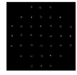
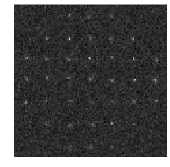
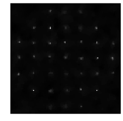
Figure 1: (a) An example simulated noiseless Shack-Hartmann wavefront sensor image, (b) with photon and readout noise added, (c) after noise removal using TVM.

In §2 we provide details of the TVM algorithm that we have investigated, and of the investigations that we have performed. In §3 we present our results, including on-sky measurements, and we conclude in §4.

2 Total variation minimisation model and application details

We use a convergent algorithm developed by Chambolle (2004) for the minimisation of total variation of an image. This algorithm has applications beyond image noise removal, for example image scaling; here however we concentrate only on noise removal.

It is assumed that an observed image, $g$ is the addition of an a priori piecewise smooth (or with little oscillation) image, $u$ and a random Gaussian noise of estimated variance $\sigma^{2}$. Therefore the original image is estimated by solving (Chambolle, 2004)

$$\mathrm{min}\left(||u-g||^{2}=N^{2}\sigma^{2}\right)$$ (1)

where $N^{2}$ is the number of pixels.

Throughout this paper, we consider noise reduction applied to individual sub-apertures, rather than noise reduction applied to the whole wavefront sensor image, because this is of most relevance to an on-sky situation: within an AO real-time control system, system latency is reduced (and hence performance improved) if individual wavefront sensor sub-apertures are processed separately, as soon as the relevant pixel data arrive at the real-time computer, rather than waiting and processing a whole frame at once. The ability to access the camera pixel stream depends somewhat on camera mode; however with the CANARY AO system (Myers et al., 2008) and many others, camera customisation, interface development, and custom software has made this possible. CANARY uses the Durham AO real-time controller (DARC) for wavefront control (Basden et al., 2010; Basden & Myers, 2012) which is optimised for low latency operation, and has the ability to process sub-apertures individually once pixels become available. We have therefore implemented the TVM algorithm within this system (which we discuss in §2.2), applying TVM on a per-sub-aperture basis.

2.1 Monte-Carlo simulation of total variation minimisation performance

There are many parameters that need to be considered when investigating sub-aperture slope estimation improvement, including the size of the spots (determined by optics and atmospheric conditions), the signal level of the target, detector readout noise, and the number of pixels within each sub-aperture.

We investigate performance of the noise removal algorithm spanning this parameter space using Monte-Carlo simulation techniques. Our procedure is as follows:

1. A sub-aperture spot is generated at a random, known, position ($S_{\textrm{true}}$).

2. Noise (photon and readout) is added.

3. Spot position is estimated using a centre of gravity algorithm ($S_{\textrm{sys}}$).

4. TVM is applied to the image.

5. Spot position is estimated using a centre of gravity algorithm ($S_{\textrm{tvm}}$).

6. Steps 1–5 are repeated many ($N$) times.

7. The performance metric is calculated.

The performance metric is given by

$$R=\frac{\sum_{m=1}^{N}|\left(S_{\textrm{true}}(m)-S(m)\right)|}{N}$$ (2)

where $N$ is the number of measurements taken and $S(m)$ is the $m^{th}$ individual slope measurement measured with the $m^{th}$ Monte-Carlo realisation, either the true position, or the estimated position (with noise added, $S_{\textrm{sys}}$, and after application of noise removal, $S_{\textrm{tvm}}$). In essence, the absolute offset between estimated and true positions are computed, and the mean offset calculated over ten thousand realisations. We refer to $R$ as the slope error, or slope estimation accuracy, and to $S_{\textrm{sys}}$ as the “No tvm” case.

We consider signal levels from high light level, down to very low (10 photons per sub-aperture i.e. too low for good AO correction, but still of academic interest). We consider a range of detector readout noise from 0.1 to 16 electrons, which includes the parameter space for the electron multiplying CCDs (EMCCDs) and scientific CMOS (sCMOS) detectors that are candidate wavefront sensors, and also that corresponding to an electronically shuttered laser guide star wavefront sensor that was used with CANARY. Sub-aperture sizes are considered from $8\times 8$ to $16\times 16$ pixels, corresponding to the sizes used for CANARY, and also those that are likely for wide-field Extremely Large Telescope (ELT)-scale AO instruments. Spot sizes are investigated ranging from Nyquist sampled, to spots with a FWHM of about four pixels, i.e. towards the practical upper size limit with which a typical AO system would work.

In conjunction with the noise removal algorithm under consideration here, we use a background subtraction algorithm based on brightest pixels (Basden et al., 2012), which sets the image background threshold level (both noisy and denoised) at a level such that a given number of image pixels remain above this threshold in each sub-aperture. When investigating performance, we use the number of retained image pixels that gives best performance.

2.2 On-sky testing of total variation minimisation

We have implemented the TVM algorithm within the DARC system that is used by CANARY. This is a dynamically loadable modular control system, and so the introduction of new algorithms does not require a modification of the core system, and these algorithms can be loaded and unloaded from the real-time system without affecting its subsequent operation, making it ideal for algorithm development.

Our implementation includes three adjustable parameters, which can be altered on a sub-aperture basis (allowing optimised operation with wavefront sensors where the spot point spread function (PSF) varies across the sensor, for example differing elongation when using laser guide stars). These are the “strength” (estimated noise standard deviation) of the noise removal, the tolerance level (at which the image is considered denoised), and the maximum number of iterations allowed (to avoid significant increase to AO system latency). The maximum number of iterations is set to a number greater than that typically required for convergence (in which case, the algorithm does not perform all iterations); it serves to prevent real-time system jitter in rare cases where the algorithm is not converging quickly.

During these tests, we operate CANARY in a single conjugate AO (SCAO) mode, using a single on-axis wavefront sensor, and interleave processing with and without TVM while measuring performance. Strehl ratio of the AO corrected image is our performance metric, computed on-axis using standard CANARY tools (Gendron et al., 2011).

3 Discussion of performance improvements using TVM

Accuracy of Shack-Hartmann slope estimation has been investigated in simulation, comparing noisy and denoised Shack-Hartmann spots. Fig. 2 shows a comparison of a simulated noisy and denoised Shack-Hartmann spot. In this figure, it is clearly evident that the TVM algorithm is effective at reducing the noise within this image.

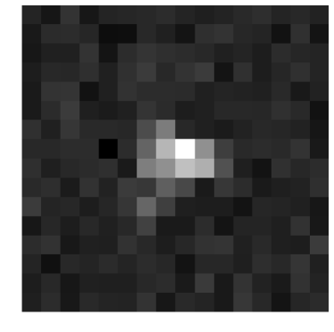
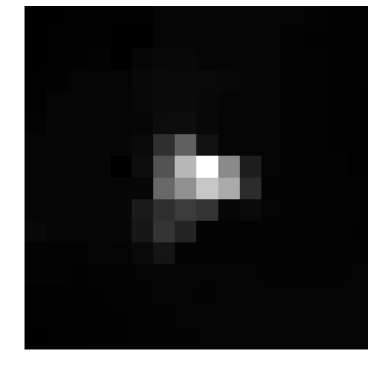
Figure 2: A comparison showing a noisy Shack-Hartmann spot, and the same image after application of the TVM algorithm.

3.1 Performance as a function of spot size

The size of a Shack-Hartmann spot determines, for a given flux level, the intensity level of the brightest pixels, since incident flux is spread over the spot. Fig. 3 shows performance as a function of signal level for different spot sizes, processed both with and without TVM. Here, a $16\times 16$ sub-aperture has been used, with 0.1 electron readout noise. From this figure, it is evident that smaller spot sizes benefit most from TVM, since the difference between the noisy and denoised cases is largest. When using TVM, a reduction in signal level by a factor of between 2–3 is possible while still maintaining the non-TVM performance level, i.e. guide star magnitude can be decreased by up to one astronomical order of magnitude when using TVM.

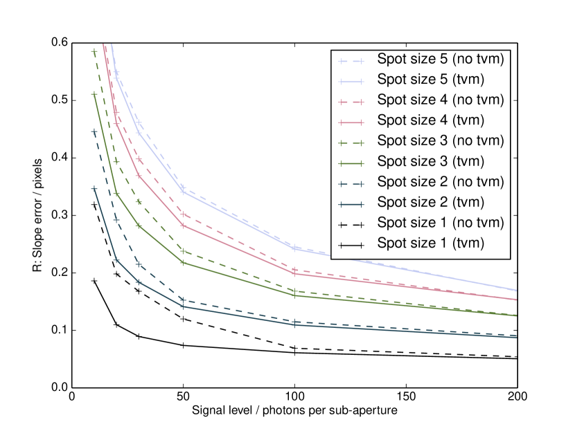
Figure 3: A figure showing Shack-Hartmann slope estimation error as a function of signal level for cases with different Shack-Hartmann spot sizes, given as a function of Nyquist sampled size in the legend. Solid lines show performance with TVM, while dashed lines are without. Uncertainties are at the 1% level and are not shown for clarity.

3.2 Performance as a function of sub-aperture size

For a given spot size, a larger sub-aperture will contain a larger number of pixels with just noise (i.e. negligible useful signal). However, in some cases, a large sub-aperture may be necessary, for example in open-loop AO systems, where a wide-field of view is required to detect large spot motions. Fig. 4 shows slope estimation error as a function of signal level, for different sub-aperture sizes. Here it is interesting to note that in the denoised case (with TVM), performance is essentially unrelated to sub-aperture size, since the TVM is successfully removing the background noise. However, in the noisy cases, performance gets worse as sub-aperture size increases as expected due to the presence of an increased number of noisy pixels. In this figure, readout noise is set at 0.1 electrons, and the Shack-Hartmann spot is Nyquist sampled.

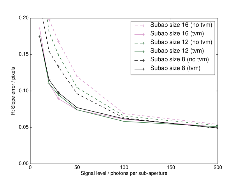
Figure 4: A figure showing Shack-Hartmann slope estimation error as a function of signal level for different sized sub-apertures, with the linear dimension given in the legend. Solid lines show performance with TVM, while dashed lines are without. Uncertainties are at the 1% level and are not shown for clarity.

3.3 Performance at low signal-to-noise ratios

Fig. 5 shows performance as a function of signal level for different wavefront sensor readout noise, for a $16\times 16$ pixel sub-aperture with a Nyquist sampled spot. Here it can be seen that as signal level is reduced, the slope error ($R$) in cases without TVM increases faster than with. At certain signal levels, using TVM allows operation at light levels a factor of 2–3 times lower than without TVM, whilst achieving the same slope estimation accuracy. For example, with a readout noise of 0.1 electrons, a signal level of 30 photons with TVM gives the same performance as 80 photons without TVM.

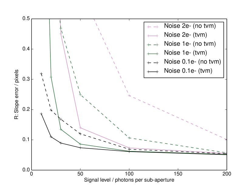
Figure 5: A figure showing Shack-Hartmann slope estimation error as a function of signal level for cases with different readout noise (as given in the legend). Solid lines show performance with TVM, while dashed lines are without. Uncertainties are at the 1% level and are not shown for clarity.

3.4 Discussion of background level selection using brightest pixels

So far, we have been using the number of pixels for background selection that give best performance, both for the noisy and denoised cases. However, it is useful to investigate how this background affects performance. Fig. 6 shows slope error ($R$) as a function of number of brightest pixels retained for two different signal levels (assuming 0.1 electrons readout noise, a $16\times 16$ sub-aperture and a Nyquist sampled spot). It is evident here that when there are fewer photons, TVM is effective at removing the effect of noise, so that the final slope error ($R$) is less dependent on the number of brightest pixels retained. Fig. 7 shows slope error ($R$) as a function of number of brightest pixels retained for different spot sizes. Here, it is clear that again, TVM removes some of the sensitivity to background level, since noise has effectively been removed (a signal level of 50 photons is assumed). Similarly, using the above assumptions, Fig. 8 shows slope error ($R$) at different detector readout noise levels, again displaying the improvements brought by the TVM algorithm.

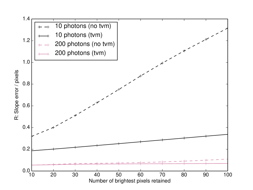
Figure 6: A figure showing slope error as a function of number of brightest pixels retained after background level removal prior to slope estimation. Results for two different light levels are shown, with and without TVM, as noted in the legend. Uncertainties are at the 1% level and are not shown for clarity.

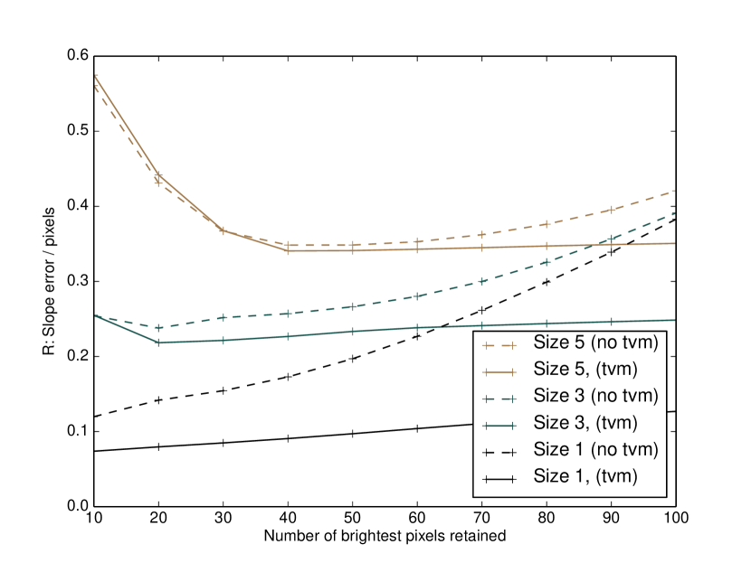
Figure 7: A figure showing slope error as a function of number of brightest pixels retained after background level removal prior to slope estimation. Results for different sub-aperture PSF spot sizes are shown, with and without TVM, as noted in the legend, where the size is the PSF oversampling factor beyond Nyquist sampled. Uncertainties are at the 1% level and are not shown for clarity.

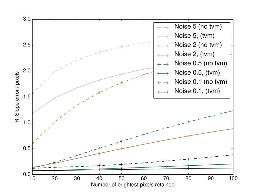
Figure 8: A figure showing slope error as a function of number of brightest pixels retained after background level removal prior to slope estimation. Results for different readout noise levels (in electrons) are shown, with and without TVM, as noted in the legend. Uncertainties are at the 1% level and are not shown for clarity.

When selecting the number of brightest pixels to retain during background level thresholding, the main consideration should be given to the size of the sub-aperture PSF. Using TVM provides a key benefit of reducing the dependency on accurate background subtraction.

3.5 Application to laser guide star elongated spots

We have also investigated the application of TVM to elongated Shack-Hartmann spots. For the results presented here, we assume a spot that is elongated by a factor of three, i.e. three times longer in one dimension than the other. Fig. 9 shows performance (slope error, $R$) as a function of signal level, for different readout noise values, both with and without TVM. It can be seen here that the benefit obtained from TVM increases with readout noise, and performance is never worse than without TVM. The performance improvements are less marked than for the natural guide star case, though the use of TVM can enable the same slope prediction performance for light levels reduced by up to about 25% for the high readout noise case with greater than three electrons.

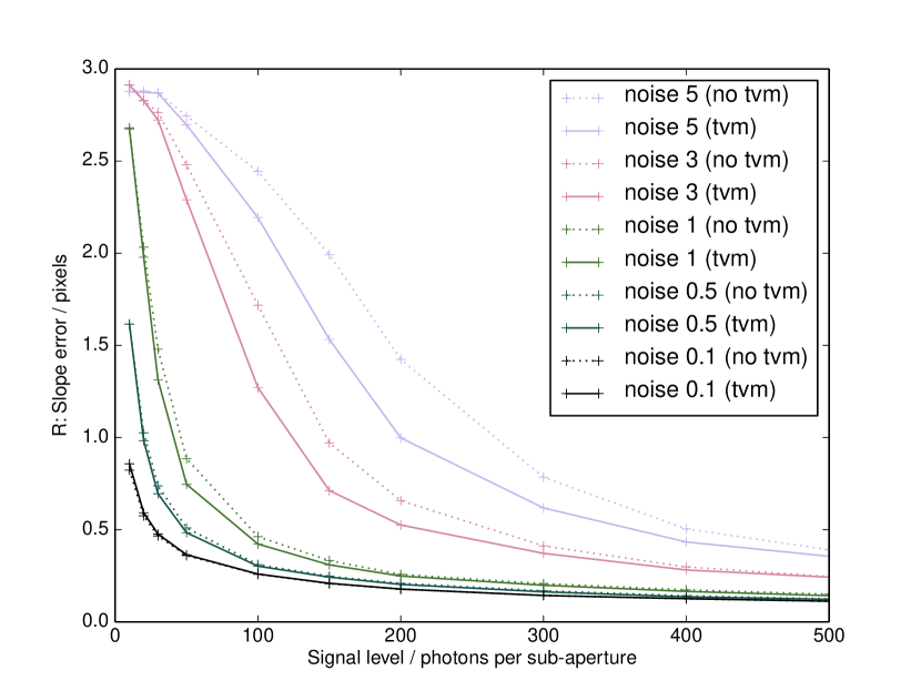
Figure 9: A figure showing predicted Shack-Hartmann slope error as a function of signal level for a $16\times 16$ pixel sub-aperture with an elongated spot PSF ($3\times$ longer than wide). Cases with and without TVM are given in the legend, for different detector readout noise. Uncertainties are at the 1% level and are not shown for clarity.

3.6 On-sky measurements

Because on-sky time was limited, we did not attempt to explore a large parameter space of seeing conditions, spot size, signal level and readout noise. Rather, we have selected a target where noise is evident within the sub-apertures (Fig. 10), and operated the CANARY AO system in SCAO mode both with and without TVM. The data presented here were taken on the night of 12th July 2014 with CANARY on the William Herschel Telescope, for just over one hour from about 3am.

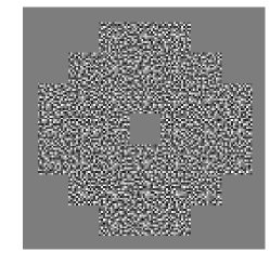
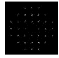
Figure 10: (a) A single frame of a wavefront sensor image obtained on-sky by the CANARY AO system at the William Herschel Telescope. (b) The noise removed using TVM with a variance of 1 (in active sub-apertures). (c) Calibrated image after TVM and background subtraction.

We have taken four sets of observations, during which the CANARY SCAO loop was closed, and H-band science images obtained. Each set of observations commenced with a measurement without TVM, and then a number of measurements (8 or 20) with different TVM strength (estimated noise standard deviation) factors (increasing monotonically from 0 to 2). Within the observation set, this was then repeated. The detector used was an EMCCD, and multiplication gain was set to maximum for the first two observation sets, and 75% for the last two, allowing the signal level to be reduced. Signal level was between 500–1000 detector counts.

Results are shown in Fig. 11, and provide evidence that this technique is able to improve AO system performance, though, due to the lack of on-sky time, this is not wholly conclusive. Mean Strehl ratios for each observation set are shown in table 1, and in each case show an improvement when using TVM. There is a large variation in performance as a function of time, which is typical of the time-varying seeing conditions commonly seen with CANARY. It should be noted that the improvement obtained using TVM is, in this case, small: it is likely that larger improvements would be seen at other signal-to-noise regimes, though this was not investigated on-sky.

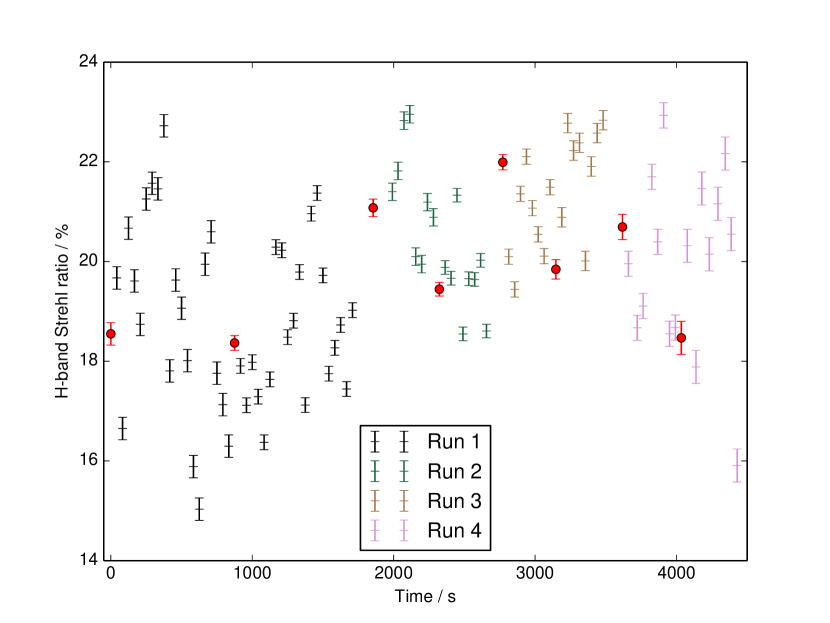
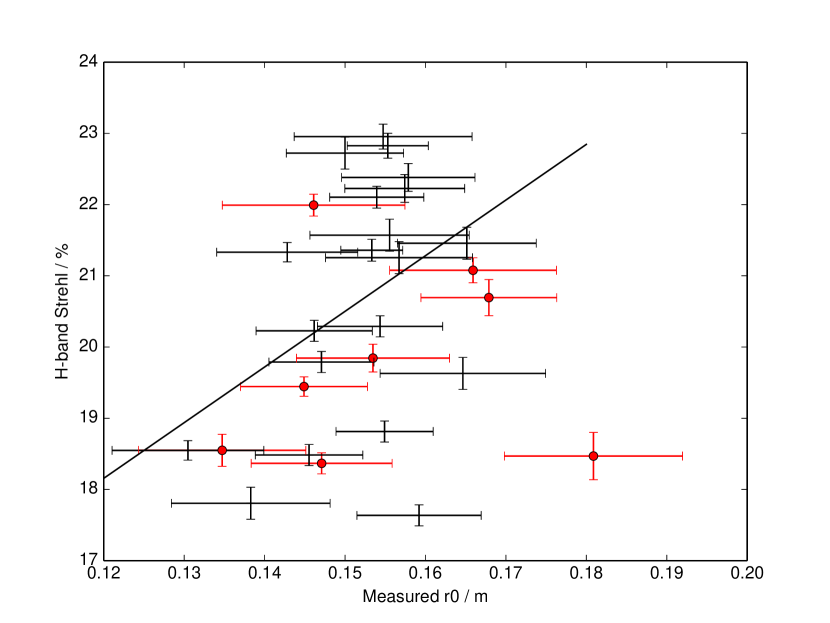
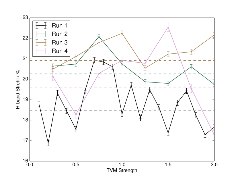
Figure 11: (a) A figure showing H-band Strehl ratio obtained with CANARY operating in SCAO mode, both with and without TVM as a function of time from first observation. The red circles show Strehl obtained without TVM, while other points are with TVM at different strengths. (b) H-band Strehl ratio as a function of $r_{0}$, with red circles representing measurements without TVM, and black crosses representing measurements with TVM. (c) H-band Strehl ratio as a function of TVM noise standard deviation estimate. The horizontal lines show Strehl obtained without TVM.

Because of the natural variability of seeing, we also show, in Fig. 11(b), the H-band Strehl ratio as a function of Fried’s parameter, $r_{0}$. In this case, $r_{0}$ is computed from reconstructed pseudo-open-loop slope measurements, which are, in turn computed from a time-series of the on-axis closed-loop wavefront slope measurements and the recorded DM actuator commands. The line fitted through these data points is the best-fit to the cases with TVM implemented (with a regression correlation 0.38). There is evidence here that the TVM performance is above the level of performance without TVM (represented by circles), indicating that the use of TVM has improved performance. However, again, there is some uncertainty, due to the lack of on-sky measurements, and so this should not be taken as conclusive: the statistical significance is low.

There is some evidence from Fig. 11(c) that using estimated noise standard deviation of around 0.8 in the TVM gives best performance (though we acknowledge that this could just be an artefact of the changing seeing conditions). Therefore, table 1 also includes the mean Strehl ratios obtained by considering only noise standard deviation estimates (TVM strength) of between 0.6 to 1.1, and shows that indeed, using TVM in this regime leads to a further increase in AO performance.

Table 1: AO system performance as given by H-band Strehl ratio (%) for CANARY operating in SCAO mode, both without and with TVM (with results averaged over all strengths, or estimated noise standard deviation, investigated) during the four different observations made (Obs). Also shown is performance using TVM with strength restricted to between 0.6–1.1.

Obs	No TVM	TVM	TVM strength 0.6–1.1
1	$18.4\pm 0.1$	$18.8\pm 1.8$	$20.0\pm 1.6$
2	$20.3\pm 1.2$	$20.5\pm 1.3$	$21.4\pm 2.0$
3	$20.9\pm 1.5$	$21.4\pm 1.1$	$22.0\pm 0.4$
4	$19.6\pm 1.6$	$20.0\pm 1.8$	$20.6\pm 1.2$

3.7 High noise wavefront sensor cameras

The wavefront sensors commonly used for laboratory AO systems typically have higher readout noise than those used on-sky, primarily for reasons of cost. We therefore investigate the performance of TVM for a sensor with a readout noise of 16 electrons, corresponding to the Imperx Bobcat model that we use with the DRAGON AO test-bench (Reeves et al., 2012). Incidentally, this sensor was also briefly used on-sky with CANARY as a substitute laser guide star (LGS) wavefront sensor (it has an electronic shuttering capability) after a fault developed in the previous sensor.

Fig. 12 shows slope error ($R$) as a function of incident signal for different sub-aperture spot sizes. As previously, the TVM algorithm provides an advantage for slope estimation, and gains up to one astronomical magnitude in performance for this sensor.

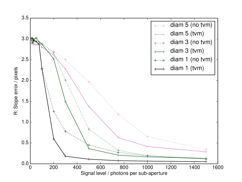
Figure 12: A figure showing Shack-Hartmann slope error as a function of signal level for a $16\times 16$ pixel sub-aperture and a detector with 16 electrons readout noise. Lines for different PSF sizes are shown (given in the legend), with the numbers corresponding to the over-sampling factor (beyond Nyquist). Cases with and without TVM are given in the legend. Uncertainties are at the 1% level and are not shown for clarity.

4 Conclusions

We have investigated the use of a TVM algorithm to improve slope estimation accuracy with Shack-Hartmann wavefront sensor images. We find that in certain situations with low signal-to-noise ratio (with appropriate signal and noise levels), the performance improvements obtained can be equivalent to gaining an astronomical magnitude in photon flux. The use of TVM never leads to a reduction in slope estimation accuracy on average. Larger sub-aperture sizes see most benefit and so this is particularly relevant for open-loop AO systems. Our investigation has shown that TVM is applicable for both natural guide star (NGS) and elongated LGS Shack-Hartmann spots. We have also presented on-sky results from the CANARY AO demonstrator instrument, which provide evidence for successful improvement of on-sky AO performance using TVM.

References

- Babcock (1953) Babcock H. W., 1953, Pub. Astron. Soc. Pacific, 65, 229
- Basden et al. (2010) Basden A., Geng D., Myers R., Younger E., 2010, Appl. Optics, 49, 6354
- Basden & Myers (2012) Basden A. G., Myers R. M., 2012, MNRAS, 424, 1483
- Basden et al. (2012) Basden A. G., Myers R. M., Gendron E., 2012, MNRAS, 419, 1628
- Chambolle (2004) Chambolle A., 2004, Journal of Mathematical Imaging and Vision, 20, 89
- Gendron et al. (2011) Gendron E., Vidal F., Brangier M., Morris T., Hubert Z., Basden A., Rousset G., Myers R., 2011, A&A, 529, L2
- Myers et al. (2008) Myers R. M., Hubert Z., Morris T. J., Gendron E., Dipper N. A., Kellerer A., Goodsell S. J., Rousset G., Younger E., Marteaud M., Basden A. G., 2008, in Society of Photo-Optical Instrumentation Engineers (SPIE) Conference Series Vol. 7015 of Presented at the Society of Photo-Optical Instrumentation Engineers (SPIE) Conference, CANARY: the on-sky NGS/LGS MOAO demonstrator for EAGLE
- Reeves et al. (2012) Reeves A. P., Myers R. M., Morris T. J., Basden A. G., Bharmal N. A., Rolt S., Bramall D. G., Dipper N. A., Younger E. J., 2012, in Society of Photo-Optical Instrumentation Engineers (SPIE) Conference Series Vol. 8447 of Society of Photo-Optical Instrumentation Engineers (SPIE) Conference Series, DRAGON: a wide-field multipurpose real time adaptive optics test bench
- Rudin et al. (1992) Rudin L., Osher S., Fatemi E., 1992, Physica D, 60, 259
- Shack (1971) Shack R. V., 1971, Journal of the Optical Society of America, 61, 656