DESY 15-037 ISSN 0418-9833
March 2015
Combination of Differential Cross-Section Measurements in Deep-Inelastic Scattering at HERA
H1 and ZEUS have published single-differential cross sections for inclusive -meson production in deep-inelastic scattering at HERA from their respective final data sets. These cross sections are combined in the common visible phase-space region of photon virtuality GeV2, electron inelasticity and the meson’s transverse momentum GeV and pseudorapidity . The combination procedure takes into account all correlations, yielding significantly reduced experimental uncertainties. Double-differential cross sections are combined with earlier data, extending the kinematic range down to GeV2. Perturbative next-to-leading-order QCD predictions are compared to the results.
Submitted to JHEP
The H1 and ZEUS Collaborations
H. Abramowicz49,a1, I. Abt36, L. Adamczyk22, M. Adamus58, V. Andreev34, S. Antonelli6, V. Aushev25,26,b21, Y. Aushev26,a2,b21, A. Baghdasaryan60, K. Begzsuren55, O. Behnke17, U. Behrens17, A. Belousov34, A. Bertolin40, I. Bloch62, E.G. Boos2, K. Borras17, V. Boudry42, G. Brandt39, V. Brisson38, D. Britzger17, I. Brock7, N.H. Brook30, R. Brugnera41, A. Bruni5, A. Buniatyan4, P.J. Bussey15, A. Bylinkin33,a3, L. Bystritskaya33, A. Caldwell36, A.J. Campbell17, K.B. Cantun Avila32, M. Capua10, C.D. Catterall37, F. Ceccopieri3, K. Cerny45, V. Chekelian36, J. Chwastowski21, J. Ciborowski57,a4, R. Ciesielski17,a5, J.G. Contreras32, A.M. Cooper-Sarkar39, M. Corradi5, F. Corriveau46, J. Cvach44, J.B. Dainton28, K. Daum59,a6, R.K. Dementiev35, R.C.E. Devenish39, C. Diaconu31, M. Dobre8, V. Dodonov17, G. Dolinska17, S. Dusini40, G. Eckerlin17, S. Egli56, E. Elsen17, L. Favart3, A. Fedotov33, J. Feltesse14, J. Ferencei20, J. Figiel21, M. Fleischer17, A. Fomenko34, B. Foster16,a7, E. Gabathuler28, G. Gach22,a8, E. Gallo16,17, A. Garfagnini41, J. Gayler17, A. Geiser17, S. Ghazaryan17, A. Gizhko17, L.K. Gladilin35, L. Goerlich21, N. Gogitidze34, Yu.A. Golubkov35, M. Gouzevitch17,a9, C. Grab63, A. Grebenyuk3, J. Grebenyuk17, T. Greenshaw28, I. Gregor17, G. Grindhammer36, G. Grzelak57, O. Gueta49, M. Guzik22, D. Haidt17, W. Hain17, R.C.W. Henderson27, J. Hladkỳ44, D. Hochman47, D. Hoffmann31, R. Hori54, R. Horisberger56, T. Hreus3, F. Huber18, Z.A. Ibrahim24, Y. Iga50, M. Ishitsuka51, A. Iudin26,a2, M. Jacquet38, X. Janssen3, F. Januschek17,a10, N.Z. Jomhari24, A.W. Jung19,a11, H. Jung17,3, I. Kadenko26, S. Kananov49, M. Kapichine13, U. Karshon47, M. Kaur9, P. Kaur9,b22, C. Kiesling36, D. Kisielewska22, R. Klanner16, M. Klein28, U. Klein17,a12, C. Kleinwort17, R. Kogler16, N. Kondrashova26,a13, O. Kononenko26, Ie. Korol17, I.A. Korzhavina35, P. Kostka28, A. Kotański23, U. Kötz17, N. Kovalchuk16, H. Kowalski17, J. Kretzschmar28, K. Krüger17, B. Krupa21, O. Kuprash17, M. Kuze51, M.P.J. Landon29, W. Lange62, P. Laycock28, A. Lebedev34, B.B. Levchenko35, S. Levonian17, A. Levy49, V. Libov17, S. Limentani41, K. Lipka17,b23, M. Lisovyi17, B. List17, J. List17, E. Lobodzinska17, B. Lobodzinski36, B. Löhr17, E. Lohrmann16, A. Longhin40,a14, D. Lontkovskyi17, O.Yu. Lukina35, I. Makarenko17, E. Malinovski34, J. Malka17, H.-U. Martyn1, S.J. Maxfield28, A. Mehta28, S. Mergelmeyer7, A.B. Meyer17, H. Meyer59, J. Meyer17, S. Mikocki21, F. Mohamad Idris24,a15, A. Morozov13, N. Muhammad Nasir24, K. Müller64, V. Myronenko17,b24, K. Nagano54, Th. Naumann62, P.R. Newman4, C. Niebuhr17, T. Nobe51, D. Notz17,†, G. Nowak21, R.J. Nowak57, J.E. Olsson17, Yu. Onishchuk26, D. Ozerov17, P. Pahl17, C. Pascaud38, G.D. Patel28, E. Paul7, E. Perez14,a16, W. Perlański57,a17, A. Petrukhin17, I. Picuric43, H. Pirumov17, D. Pitzl17, R. Plačakytė17,b23, B. Pokorny45, N.S. Pokrovskiy2, R. Polifka45,a18, M. Przybycień22, V. Radescu17,b23, N. Raicevic43, T. Ravdandorj55, P. Reimer44, E. Rizvi29, P. Robmann64, P. Roloff17,a16, R. Roosen3, A. Rostovtsev33, M. Rotaru8, I. Rubinsky17, S. Rusakov34, M. Ruspa53, D. Šálek45, D.P.C. Sankey11, M. Sauter18, E. Sauvan31,a19, D.H. Saxon15, M. Schioppa10, W.B. Schmidke36,a20, S. Schmitt17, U. Schneekloth17, L. Schoeffel14, A. Schöning18, T. Schörner-Sadenius17, F. Sefkow17, L.M. Shcheglova35, R. Shevchenko26,a2, O. Shkola26,a21, S. Shushkevich17, Yu. Shyrma25, I. Singh9,b25, I.O. Skillicorn15, W. Słomiński23,b26, A. Solano52, Y. Soloviev17,34, P. Sopicki21, D. South17, V. Spaskov13, A. Specka42, L. Stanco40, M. Steder17, N. Stefaniuk17, A. Stern49, P. Stopa21, U. Straumann64, T. Sykora3,45, J. Sztuk-Dambietz16,a10, D. Szuba16, J. Szuba17, E. Tassi10, P.D. Thompson4, K. Tokushuku54,a22, J. Tomaszewska57,a23, D. Traynor29, A. Trofymov26,a13, P. Truöl64, I. Tsakov48, B. Tseepeldorj55,a24, T. Tsurugai61, M. Turcato16,a10, O. Turkot17,b24, J. Turnau21, T. Tymieniecka58, A. Valkárová45, C. Vallée31, P. Van Mechelen3, Y. Vazdik34, A. Verbytskyi36, O. Viazlo26, R. Walczak39, W.A.T. Wan Abdullah24, D. Wegener12, K. Wichmann17,b24, M. Wing30,a25, G. Wolf17, E. Wünsch17, S. Yamada54, Y. Yamazaki54,a26, J. Žáček45, N. Zakharchuk26,a13, A.F. Żarnecki57, L. Zawiejski21, O. Zenaiev17, Z. Zhang38, B.O. Zhautykov2, N. Zhmak25,b21, R. Žlebčík45, H. Zohrabyan60, F. Zomer38 and D.S. Zotkin35
- 1
-
I. Physikalisches Institut der RWTH, Aachen, Germany
- 2
-
Institute of Physics and Technology of Ministry of Education and Science of Kazakhstan, Almaty, Kazakhstan
- 3
-
Inter-University Institute for High Energies ULB-VUB, Brussels and Universiteit Antwerpen, Antwerpen, Belgiumb1
- 4
-
School of Physics and Astronomy, University of Birmingham, Birmingham, UKb2
- 5
-
INFN Bologna, Bologna, Italyb3
- 6
-
University and INFN Bologna, Bologna, Italyb3
- 7
-
Physikalisches Institut der Universität Bonn, Bonn, Germanyb4
- 8
-
National Institute for Physics and Nuclear Engineering (NIPNE) , Bucharest, Romaniab5
- 9
-
Panjab University, Department of Physics, Chandigarh, India
- 10
-
Calabria University, Physics Department and INFN, Cosenza, Italyb3
- 11
-
STFC, Rutherford Appleton Laboratory, Didcot, Oxfordshire, UKb2
- 12
-
Institut für Physik, TU Dortmund, Dortmund, Germanyb6
- 13
-
Joint Institute for Nuclear Research, Dubna, Russia
- 14
-
CEA, DSM/Irfu, CE-Saclay, Gif-sur-Yvette, France
- 15
-
School of Physics and Astronomy, University of Glasgow, Glasgow, United Kingdomb2
- 16
-
Institut für Experimentalphysik, Universität Hamburg, Hamburg, Germanyb6,b7
- 17
-
Deutsches Elektronen-Synchrotron DESY, Hamburg, Germany
- 18
-
Physikalisches Institut, Universität Heidelberg, Heidelberg, Germanyb6
- 19
-
Kirchhoff-Institut für Physik, Universität Heidelberg, Heidelberg, Germanyb6
- 20
-
Institute of Experimental Physics, Slovak Academy of Sciences, Košice, Slovak Republicb8
- 21
-
The Henryk Niewodniczanski Institute of Nuclear Physics, Polish Academy of Sciences, Krakow, Polandb9,b15
- 22
-
AGH-University of Science and Technology, Faculty of Physics and Applied Computer Science, Krakow, Polandb9
- 23
-
Department of Physics, Jagellonian University, Krakow, Poland
- 24
-
National Centre for Particle Physics, Universiti Malaya, 50603 Kuala Lumpur, Malaysiab10
- 25
-
Institute for Nuclear Research, National Academy of Sciences, Kyiv, Ukraine
- 26
-
Department of Nuclear Physics, National Taras Shevchenko University of Kyiv, Kyiv, Ukraine
- 27
-
Department of Physics, University of Lancaster, Lancaster, UKb2
- 28
-
Department of Physics, University of Liverpool, Liverpool, UKb2
- 29
-
School of Physics and Astronomy, Queen Mary, University of London, London, UKb2
- 30
-
Physics and Astronomy Department, University College London, London, United Kingdomb2
- 31
-
Aix Marseille Université, CNRS/IN2P3, CPPM UMR 7346, 13288 Marseille, France
- 32
-
Departamento de Fisica Aplicada, CINVESTAV, Mérida, Yucatán, Méxicob11
- 33
-
Institute for Theoretical and Experimental Physics, Moscow, Russiab12
- 34
-
Lebedev Physical Institute, Moscow, Russia
- 35
-
Lomonosov Moscow State University, Skobeltsyn Institute of Nuclear Physics, Moscow, Russiab13
- 36
-
Max-Planck-Institut für Physik, München, Germany
- 37
-
Department of Physics, York University, Ontario, Canada M3J 1P3b14
- 38
-
LAL, Université Paris-Sud, CNRS/IN2P3, Orsay, France
- 39
-
Department of Physics, University of Oxford, Oxford, United Kingdomb2
- 40
-
INFN Padova, Padova, Italyb3
- 41
-
Dipartimento di Fisica e Astronomia dell’ Università and INFN, Padova, Italyb3
- 42
-
LLR, Ecole Polytechnique, CNRS/IN2P3, Palaiseau, France
- 43
-
Faculty of Science, University of Montenegro, Podgorica, Montenegrob16
- 44
-
Institute of Physics, Academy of Sciences of the Czech Republic, Praha, Czech Republicb17
- 45
-
Faculty of Mathematics and Physics, Charles University, Praha, Czech Republicb17
- 46
-
Department of Physics, McGill University, Montréal, Québec, Canada H3A 2T8b14
- 47
-
Department of Particle Physics and Astrophysics, Weizmann Institute, Rehovot, Israel
- 48
-
Institute for Nuclear Research and Nuclear Energy, Sofia, Bulgaria
- 49
-
Raymond and Beverly Sackler Faculty of Exact Sciences, School of Physics, Tel Aviv University, Tel Aviv, Israelb18
- 50
-
Polytechnic University, Tokyo, Japanb19
- 51
-
Department of Physics, Tokyo Institute of Technology, Tokyo, Japanb19
- 52
-
Università di Torino and INFN, Torino, Italyb3
- 53
-
Università del Piemonte Orientale, Novara, and INFN, Torino, Italyb3
- 54
-
Institute of Particle and Nuclear Studies, KEK, Tsukuba, Japanb19
- 55
-
Institute of Physics and Technology of the Mongolian Academy of Sciences, Ulaanbaatar, Mongolia
- 56
-
Paul Scherrer Institut, Villigen, Switzerland
- 57
-
Faculty of Physics, University of Warsaw, Warsaw, Poland
- 58
-
National Centre for Nuclear Research, Warsaw, Poland
- 59
-
Fachbereich C, Universität Wuppertal, Wuppertal, Germany
- 60
-
Yerevan Physics Institute, Yerevan, Armenia
- 61
-
Meiji Gakuin University, Faculty of General Education, Yokohama, Japanb19
- 62
-
Deutsches Elektronen-Synchrotron DESY, Zeuthen, Germany
- 63
-
Institut für Teilchenphysik, ETH, Zürich, Switzerlandb20
- 64
-
Physik-Institut der Universität Zürich, Zürich, Switzerlandb20
- †
-
Deceased
- a1
-
Also at Max Planck Institute for Physics, Munich, Germany, External Scientific Member
- a2
-
Member of National Technical University of Ukraine, Kyiv Polytechnic Institute, Kyiv, Ukraine
- a3
-
Also at Moscow Institute of Physics and Technology, Moscow, Russia
- a4
-
Also at Łódź University, Poland
- a5
-
Now at Rockefeller University, New York, NY 10065, USA
- a6
-
Also at Rechenzentrum, Universität Wuppertal, Wuppertal, Germany
- a7
-
Alexander von Humboldt Professor; also at DESY and University of Oxford
- a8
-
Now at School of Physics and Astronomy, University of Birmingham, UK
- a9
-
Also at IPNL, Université Claude Bernard Lyon 1, CNRS/IN2P3, Villeurbanne, France
- a10
-
Now at European X-ray Free-Electron Laser facility GmbH, Hamburg, Germany
- a11
-
Now at Fermilab, Chicago, United States
- a12
-
Now at University of Liverpool, United Kingdom
- a13
-
Now at DESY ATLAS group
- a14
-
Now at LNF, Frascati, Italy
- a15
-
Also at Agensi Nuklear Malaysia, 43000 Kajang, Bangi, Malaysia
- a16
-
Now at CERN, Geneva, Switzerland
- a17
-
Member of Łódź University, Poland
- a18
-
Also at Department of Physics, University of Toronto, Toronto, Ontario, Canada M5S 1A7
- a19
-
Also at LAPP, Université de Savoie, CNRS/IN2P3, Annecy-le-Vieux, France
- a20
-
Now at BNL, USA
- a21
-
Member of National University of Kyiv - Mohyla Academy, Kyiv, Ukraine
- a22
-
Also at University of Tokyo, Japan
- a23
-
Now at Polish Air Force Academy in Deblin
- a24
-
Also at Ulaanbaatar University, Ulaanbaatar, Mongolia
- a25
-
Also at Universität Hamburg and supported by DESY and the Alexander von Humboldt Foundation
- a26
-
Now at Kobe University, Japan
- b1
-
Supported by FNRS-FWO-Vlaanderen, IISN-IIKW and IWT and by Interuniversity Attraction Poles Programme, Belgian Science Policy
- b2
-
Supported by the UK Science and Technology Facilities Council, and formerly by the UK Particle Physics and Astronomy Research Council
- b3
-
Supported by the Italian National Institute for Nuclear Physics (INFN)
- b4
-
Supported by the German Federal Ministry for Education and Research (BMBF), under contract No. 05 H09PDF
- b5
-
Supported by the Romanian National Authority for Scientific Research under the contract PN 09370101
- b6
-
Supported by the Bundesministerium für Bildung und Forschung, FRG, under contract numbers 05H09GUF, 05H09VHC, 05H09VHF, 05H16PEA
- b7
-
Supported by the SFB 676 of the Deutsche Forschungsgemeinschaft (DFG)
- b8
-
Supported by VEGA SR grant no. 2/7062/ 27
- b9
-
Supported by the National Science Centre under contract No. DEC-2012/06/M/ST2/00428
- b10
-
Supported by HIR grant UM.C/625/1/HIR/149 and UMRG grants RU006-2013, RP012A-13AFR and RP012B-13AFR from Universiti Malaya, and ERGS grant ER004-2012A from the Ministry of Education, Malaysia
- b11
-
Supported by CONACYT, México, grant 48778-F
- b12
-
Russian Foundation for Basic Research (RFBR), grant no 1329.2008.2 and Rosatom
- b13
-
Supported by RF Presidential grant N 3042.2014.2 for the Leading Scientific Schools and by the Russian Ministry of Education and Science through its grant for Scientific Research on High Energy Physics
- b14
-
Supported by the Natural Sciences and Engineering Research Council of Canada (NSERC)
- b15
-
Partially Supported by Polish Ministry of Science and Higher Education, grant DPN/N168/DESY/2009
- b16
-
Partially Supported by Ministry of Science of Montenegro, no. 05-1/3-3352
- b17
-
Supported by the Ministry of Education of the Czech Republic under the project INGO-LG14033
- b18
-
Supported by the Israel Science Foundation
- b19
-
Supported by the Japanese Ministry of Education, Culture, Sports, Science and Technology (MEXT) and its grants for Scientific Research
- b20
-
Supported by the Swiss National Science Foundation
- b21
-
Supported by DESY, Germany
- b22
-
Also funded by Max Planck Institute for Physics, Munich, Germany, now at Sant Longowal Institute of Engineering and Technology, Longowal, Punjab, India
- b23
-
Supported by the Initiative and Networking Fund of the Helmholtz Association (HGF) under the contract VH-NG-401 and S0-072
- b24
-
Supported by the Alexander von Humboldt Foundation
- b25
-
Also funded by Max Planck Institute for Physics, Munich, Germany, now at Sri Guru Granth Sahib World University, Fatehgarh Sahib, India
- b26
-
Partially supported by the Polish National Science Centre projects DEC-2011/01/B/ST2/03643 and DEC-2011/03/B/ST2/00220
1 Introduction
Measurements of open charm production in deep-inelastic electron111In this paper, ‘electron’ is used to denote both electron and positron if not stated otherwise. –proton scattering (DIS) at HERA provide important input for stringent tests of the theory of strong interactions, quantum chromodynamics (QCD). Previous measurements [1, 2, 3, 4, 5, 6, 7, 8, 9, 10, 11, 12, 13, 14, 15, 16, 17, 18, 19, 20] have demonstrated that charm quarks are predominantly produced by the boson–gluon-fusion process, , whereby charm production becomes sensitive to the gluon distribution in the proton. Measurements have been obtained both from the HERA-I (1992–2000) and HERA-II (2003–2007) data-taking periods.
Different techniques have been applied at HERA to measure open-charm production in DIS. The full reconstruction of or mesons [1, 2, 3, 4, 5, 6, 10, 11, 12, 15, 16, 18, 20], the long lifetime of heavy flavoured hadrons [7, 8, 9, 12, 14, 17, 19] or their semi-leptonic decays [13] are exploited. After extrapolation from the visible to the full phase space, most of these data have already been combined [21] at the level of the reduced cross-sections and have provided a consistent determination of the charm contribution to the proton structure functions, a measurement of the charm-quark mass and improved predictions for - and -production cross sections at the LHC. However, the extrapolation procedure requires theoretical assumptions, which lead to theoretical uncertainties comparable in size to the experimental uncertainties [21]. Moreover, this combination was restricted to inclusive DIS variables only, such as the photon virtuality, , and the inelasticity, . Alternatively, the measured cross sections can be combined directly in the visible phase space. In this case, dependences on the theoretical input are minimised and the charm production mechanism can be explored in terms of other variables. Such a combination, however, is possible only for data with the same final state, covering a common visible phase space. The recently published differential cross-section measurements by H1 [18, 15] and ZEUS [20] for inclusive -meson production fulfil this requirement. The analysis of fully reconstructed mesons also offers the best signal-to-background ratio and small statistical uncertainties.
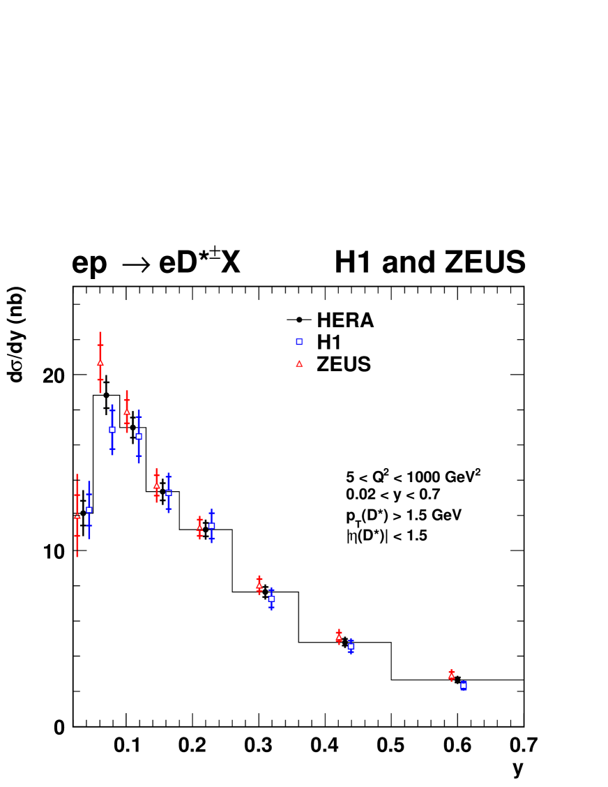
In this paper, visible -production cross sections [18, 15, 20, 6] at the centre-of-mass energy GeV are combined such that one consistent HERA data set is obtained and compared directly to differential next-to-leading-order (NLO) QCD predictions. The combination is based on the procedure described elsewhere [21, 22, 23, 24], accounting for all correlations in the uncertainties. This yields a significant reduction of the overall uncertainties of the measurements. The possibility to describe all measurements both in shape and normalisation with a single set of theory parameter values is also investigated and interpreted in terms of future theory improvements.
The paper is organised as follows. In Section 2 the theoretical framework is briefly introduced that is used for applying phase-space corrections to the input data sets prior to combination and for providing NLO QCD predictions to be compared to the data. The data samples used for the combination are detailed in Section 3 and the combination procedure is described in Section 4. The combined single- and double-differential cross sections are presented in Section 5 together with a comparison of NLO QCD predictions to the data.
2 Theoretical predictions
The massive fixed-flavour-number scheme (FFNS) [25] is used for theoretical predictions, since it is the only scheme for which fully differential NLO calculations [26] are available. The cross-section predictions for production presented in this paper are obtained using the HVQDIS program [26] which provides NLO QCD () calculations in the 3-flavour FFNS for charm and beauty production in DIS. These predictions are used both for small phase-space corrections of the data, due to slightly different binning schemes and kinematic cuts, and for comparison to data.
The following parameters are used in the calculations and are varied within certain limits to estimate the uncertainties associated with the predictions:
-
•
The renormalisation and factorisation scales are taken as . The scales are varied simultaneously up or down by a factor of two for the phase-space corrections where only the shape of the differential cross sections is relevant. For absolute predictions, the scales are changed independently to and times their nominal value.
-
•
The pole mass of the charm quark is set to GeV. This variation also affects the values of the renormalisation and factorisation scales.
-
•
For the strong coupling constant the value is chosen [21] which corresponds to .
-
•
The proton parton density functions (PDFs) are described by a series of FFNS variants of the HERAPDF1.0 set [24] at NLO determined within the HERAFitter [27] framework, similar to those used in the charm combination paper [21]. Charm measurements were not included in the determination of these PDF sets. For all parameter settings used here, the corresponding PDF set is used. By default, the scales for the charm contribution to the inclusive data in the PDF determination were chosen to be consistent with the factorisation scale used in HVQDIS, while the renormalisation scale in HVQDIS was decoupled from the scale used in the PDF extraction, except in the cases where the factorisation and renormalisation scales were varied simultaneously. As a cross check, the renormalisation scales for both heavy- and light-quark contributions are varied simultaneously in HVQDIS and in the PDF determination, keeping the factorisation scales fixed. The result lies well within the quoted uncertainties. The cross sections are also evaluated with 3-flavour NLO versions of the ABM [28] and MSTW [29] PDF sets. The differences are found to be negligible compared to those from varying other parameters, such that no attempt for coverage of all possible PDFs is made.
The NLO calculation performed by the HVQDIS program yields differential cross sections for charm quarks. These predictions are converted to -meson cross sections by applying the fragmentation model described in a previous publication [21]. This model is based on the fragmentation function of Kartvelishvili et al. [30] which provides a probability density function for the fraction of the charm-quark momentum transferred to the meson. The function is controlled by a single fragmentation parameter, . Different values of [21] are used for different regions of the invariant mass, , of the photon–parton centre-of-mass system. The boundary GeV2 between the first two regions is one of the parameter variations. The boundary GeV2 between the second and third region remains fixed. The model also implements a transverse-fragmentation component by assigning to the meson a transverse momentum, , with respect to the charm-quark direction [21]. The following parameters are used in the calculations together with the corresponding variations for estimating the uncertainties of the NLO predictions related to fragmentation:
The small beauty contribution to the signal needs a detailed treatment of the hadron decay to mesons and is therefore obtained from NLO QCD predictions for beauty hadrons convoluted with decay tables to mesons and decay kinematics obtained from EvtGen [32]. The parameters for the calculations and the uncertainties are:
-
•
The renormalisation and factorisation scales are varied in the same way as described above for charm. The variations are applied simultaneously for the calculation of the charm and beauty cross-section uncertainties.
-
•
The pole mass of the beauty quark is set to GeV.
- •
-
•
The fraction of beauty hadrons decaying into mesons is set to
[35]. -
•
The proton structure is described by the same PDF set (3-flavour scheme) used for the charm cross-section predictions.
The total theoretical uncertainties are obtained by adding all individual contributions in quadrature.
3 Data samples for cross-section combinations
The H1[36, 37, 38] and ZEUS [39] detectors were general purpose instruments which consisted of tracking systems surrounded by electromagnetic and hadronic calorimeters and muon detectors. The most important detector components for the measurements combined in this paper are the central tracking detectors (CTD) operated inside solenoidal magnetic fields of T (H1) and T (ZEUS) and the electromagnetic sections of the calorimeters. The CTD of H1 [37] (ZEUS [40]) measured charged particle trajectories in the polar angular range222In both experiments a right-handed coordinate system is employed with the axis pointing in the nominal proton-beam direction, referred to as “forward direction”, and the axis pointing towards the centre of HERA. The origin of the coordinate system is defined by the nominal interaction point in the case of H1 and by the centre of the CTD in the case of ZEUS. of . In both detectors the CTDs were complemented with high-resolution silicon vertex detectors: a system of three silicon detectors for H1, consisting of the Backward Silicon Tracker [41], the Central Silicon Tracker [42] and the Forward Silicon Tracker [43], and the Micro Vertex Detector [44] for ZEUS. For charged particles passing through all active layers of the silicon vertex detectors and CTDs, transverse-momentum resolutions of (H1) and (ZEUS), with in units of GeV, have been achieved.
Each of the central tracking detectors was enclosed by a set of calorimeters comprising an inner electromagnetic and an outer hadronic section. The H1 calorimeter system consisted of the Liquid Argon calorimeter (LAr) [45] and the backward lead–scintillator calorimeter (SpaCal) [38] while the ZEUS detector was equipped with a compensating uranium–scintillator calorimeter (CAL) [46]. Most important for the analyses combined in this paper is the electromagnetic part of the calorimeters which is used to identify and measure the scattered electron. Electromagnetic energy resolutions of (LAr) [47], (SpaCal) [48] and (CAL), with in units of GeV, were achieved.
The Bethe–Heitler process, , is used by both experiments to determine the luminosity. Photons originating from this reaction were detected by photon taggers at about m downstream of the electron beam line. The integrated luminosities are known with a precision of % for the H1 measurements [18, 15] and of about % for the ZEUS measurements [20, 6, 49].
| Data set | Kinematic range | ||||||
| ( GeV2) | ( GeV) | () | |||||
| I | H1 HERA-II (medium ) | [18] | |||||
| II | H1 HERA-II (high ) | [15] | |||||
| III | ZEUS HERA-II | [20] | |||||
| IV | ZEUS 98-00 | [6] | |||||
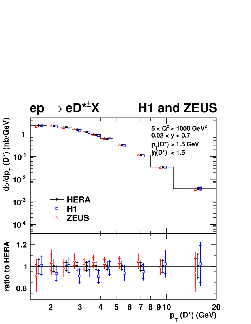
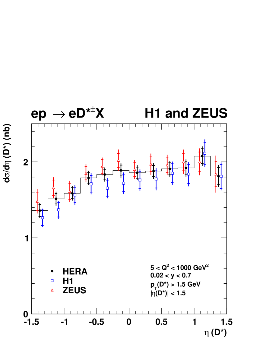
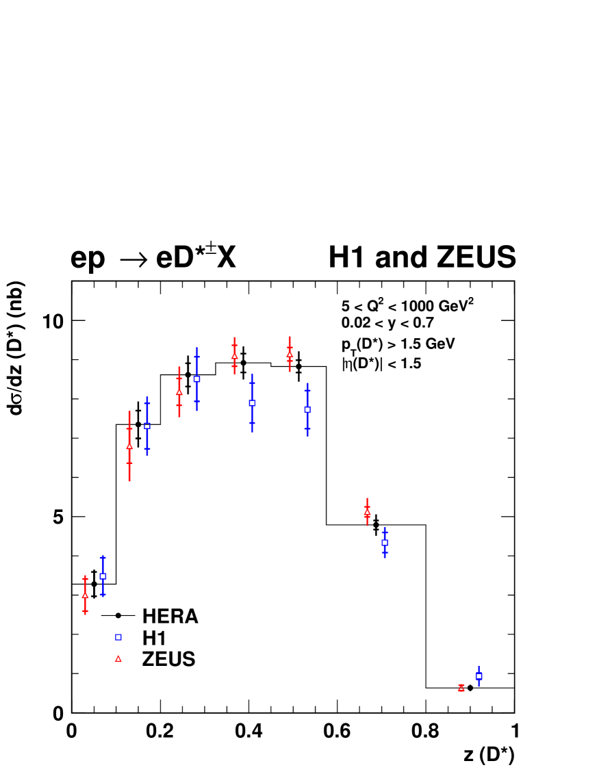
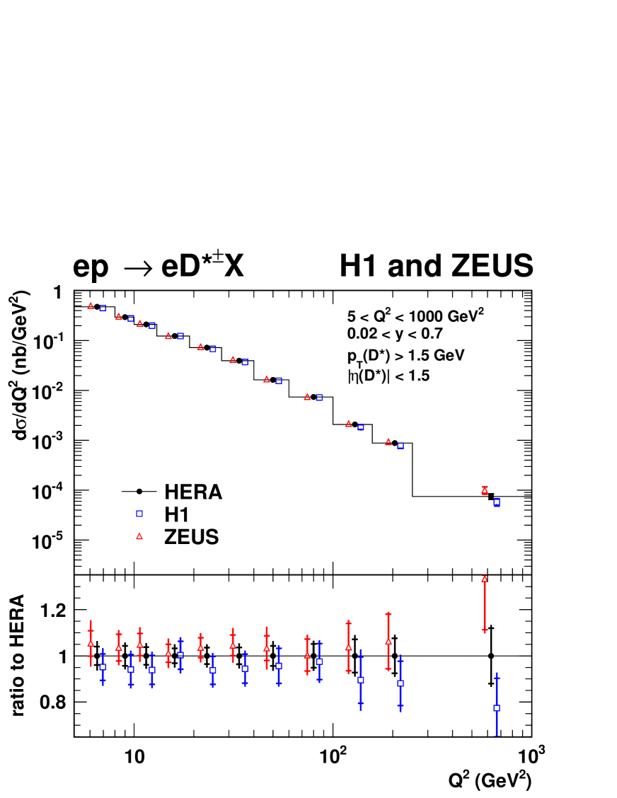
Combinations are made for single- and double-differential cross sections. In Table 1 the datasets333Of the two sets of measurements in [18], that compatible with the above cuts is chosen. used for these combinations are listed together with their visible phase-space regions and integrated luminosities. The datasets I–III are used to determine single-differential combined cross sections as a function of the meson’s transverse momentum, , pseudorapidity, , and inelasticity, , measured in the laboratory frame, and of and . The variables , and denote the energy of the meson, the component of the momentum of the meson and the incoming electron energy, respectively. Owing to beam-line modifications related to the HERA-II high-luminosity running [50] the visible phase space of these cross sections at HERA-II is restricted to GeV2, which prevents a combination with earlier cross-section measurements for which the phase space extends down to GeV2.
In the case of the double-differential cross section, , the kinematic range can be extended to lower using HERA-I measurements [10, 4, 6]. In order to minimise the use of correction factors derived from theoretical calculations, the binning scheme of such measurements has to be similar to that used for the HERA-II data. One of the HERA-I measurements, set IV of Table 1, satisfies this requirement and is therefore included in the combination of this double-differential cross section. The visible phase spaces of the combined single- and double-differential cross sections are summarised in Table 2.
The measurements to be combined for the single- and double-differential cross sections are already corrected to the Born level with a running fine-structure constant and include both the charm and beauty contributions to production. The total expected beauty contribution is small, varying from at the lowest to at the highest . The cross sections measured previously [6, 18, 15] are here corrected to the PDG value [35] of the branching ratio.
| single | double | |||
|---|---|---|---|---|
| Range in | differential cross section | |||
| (GeV2) | ||||
| (GeV) | ||||
3.1 Treatment of data sets for single-differential cross sections
In order to make the input data sets compatible with the phase space quoted in Table 2 and with each other, the following corrections are applied before the combination:
-
•
The H1 collaboration has published measurements of cross sections separately for GeV GeV2 (set I) and for GeV GeV2 (set II). Due to the limited statistics at high , a coarser binning in , , and was used in set II compared to set I. Therefore the cross section in a bin of a given observable integrated in the range GeV GeV2 is calculated according to
Here denotes the integrated visible cross section and stands for the NLO predictions obtained from HVQDIS. In this calculation both the experimental uncertainties of the visible cross section at high and the theoretical uncertainties as described in Section 2 are included. The contribution from the region GeV GeV2 to the full range amounts to % on average and reaches up to % at highest .
-
•
The bin boundaries used for the differential cross section as a function of differ between sets I, II and set III. At low this is solved by combining the cross-section measurements of the first two bins of set I into a single bin. For GeV2 no consistent binning scheme could be defined directly from the single-differential cross-section measurements. However, the measurements of the double-differential cross sections have been performed in a common binning scheme. By integrating these cross sections in , single-differential cross sections in are obtained also for GeV2 which can be used directly in the combination.
-
•
The cross-section measurements in set III are restricted to GeV while there is no such limitation in the phase space of the combination. Therefore these cross sections are corrected for the contribution from the range GeV using HVQDIS. This correction is found to be less than %.
3.2 Treatment of data sets for double-differential cross sections
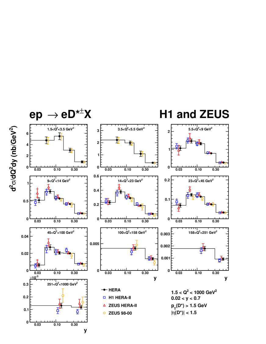
Since the restriction to the same phase space in does not apply for the combination of the double-differential cross sections in and , the HERA-I measurement, set IV, is also included in the combination. This allows an extension of the kinematic range down to . The ranges of the measurements of sets III and IV are corrected in the same way as for the single-differential cross sections.
To make the binning scheme of the HERA-I measurement compatible with that used for the HERA-II datasets, the binning for all datasets is revised. Cross sections in the new bins are obtained from the original bins using the shape of the HVQDIS predictions as described in Section 2. The new binning is given in Section 5 (Table 9). Bins are kept only if they satisfied both of the following criteria:
-
•
The predicted fraction of the cross section of the original bin contained in the kinematical overlap region in and between the original and corrected bins is greater than 50% (in most bins it is greater than 90%).
-
•
The theoretical uncertainty from the correction procedure is obtained by evaluating all uncertainties discussed in Section 2 and adding them in quadrature. The ratio of the theoretical uncertainty to the uncorrelated experimental uncertainty is required to be less than 30%.
This procedure ensures that the effect of the theoretical uncertainties on the combined data points is small. Most of the HERA-II bins are left unmodified; all of them satisfied the criteria and are kept. Out of the 31 original HERA-I bins, 26 bins satisfy the criteria and are kept. The data points removed from the combination mainly correspond to the low- region where larger bins were used for the HERA-I data.
4 Combination method
The combination of the data sets uses the minimisation method developed for the combination of inclusive DIS cross sections [22, 24], as implemented in the HERAverager program [51]. For an individual dataset the contribution to the function is defined as
| (2) |
Here is the measured value of the cross section in bin and , and are the relative correlated systematic, relative statistical and relative uncorrelated systematic uncertainties, respectively, from the original measurements. The quantities express the values of the expected combined cross section for each bin and the quantities express the shifts of the correlated systematic-uncertainty sources , in units of the standard deviation. Several data sets providing a number of measurements (index ) are represented by a total function, which is built from the sum of the functions of all data sets
| (3) |
The combined cross sections are obtained by the minimisation of with respect to and .
The averaging procedure also provides the covariance matrix of the and the uncertainties of the at the minimum. The at the minimum and their uncertainties are referred to as “shift” and “reduction”, respectively. The covariances of the are given in the form [23]. The matrix is diagonal. Its diagonal elements correspond to the covariances obtained in a weighted average performed in the absence of any correlated systematic uncertainties. The covariance matrix contributions correspond to correlated systematic uncertainties on the averaged cross sections, such that the elements of a matrix are obtained as , given a vector of systematic uncertainties. It is worth noting that, in this representation of the covariance matrix, the number of correlated systematic sources is identical to the number of correlated systematic sources in the input data sets.
In the present analysis, the correlated and uncorrelated systematic uncertainties are predominantly of multiplicative nature, i.e. they change proportionally to the central values. In equation (2) the multiplicative nature of these uncertainties is taken into account by multiplying the relative errors and by the cross-section expectation . In charm analyses the statistical uncertainty is mainly background dominated. Therefore it is treated as being independent of . For the minimisation of an iterative procedure is used as described elsewhere [23].
The systematic uncertainties obtained from the original publications were examined for their correlations. Within each data set, most of the systematic uncertainties are found to be point-to-point correlated, and are thus treated as fully correlated in the combination. In total there are correlated experimental systematic sources and theory-related uncertainty sources. A few are found to be uncorrelated and added in quadrature. For the combination of single-differential cross sections the uncorrelated uncertainties also include a theory-related uncertainty from the corrections discussed in Section 3, which varies between 0 and 10% of the total uncertainty and is added in quadrature. Asymmetric systematic uncertainties were symmetrised to the larger deviation before performing the combination. Except for the branching-ratio uncertainty, which was treated as correlated, all experimental systematic uncertainties were treated as independent between the H1 and ZEUS data sets. Since the distributions in , , , and are not statistically independent, each distribution is combined separately.
5 Combined cross sections
The results of combining the HERA-II measurements
[18, 15, 20]
as a function of , , , and are given
in Tables 3 – 7, together with their uncorrelated and correlated uncertainties444
A detailed breakdown of correlated uncertainties can be
found on
http://www.desy.de/h1zeus/dstar2015/..
The total uncertainties are obtained by adding the uncorrelated and correlated
uncertainties in quadrature.
The individual data sets and the results of the combination are shown in Figures 1 – 5. The consistency of the data sets as well as the reduction of the uncertainties are illustrated further by the insets at the bottom of Figures 1 and 4. The combinations in the different variables have a probability varying between 15% and 87%, i.e. the data sets are consistent. The systematic shift between the two input data sets is covered by the respective correlated uncertainties. The shifts and reductions of the correlated uncertainties are given in Table 8. The improvement of the total correlated uncertainty is due to small reductions of many sources. While the effective doubling of the statistics of the combined result reduces the uncorrelated uncertainties, the correlated uncertainties of the combined cross sections are reduced through cross-calibration effects between the two experiments. Typically, both effects contribute about equally to the reduction of the total uncertainty.
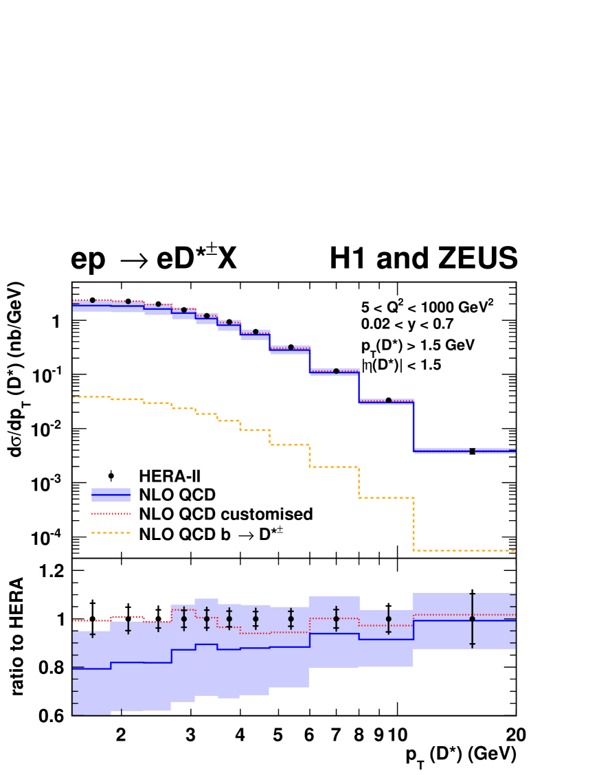
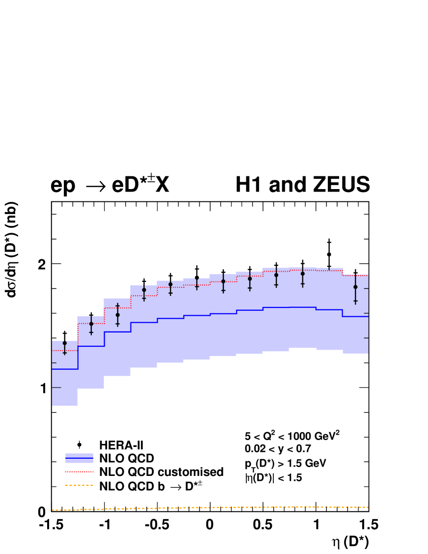
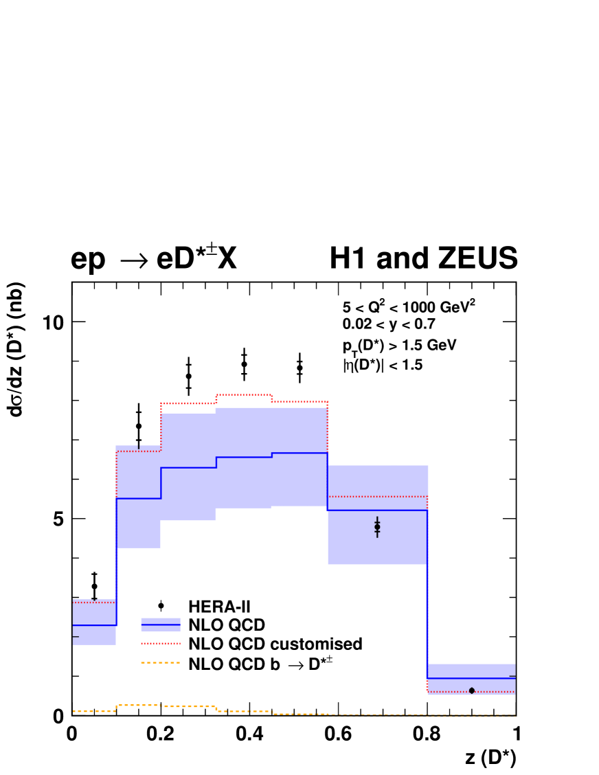
The combined cross sections as a function of
, , , and
are compared to NLO predictions555The NLO QCD prediction for the beauty contribution to production,
calculated as described in Section 2, can be found on
http://www.desy.de/h1zeus/dstar2015/.
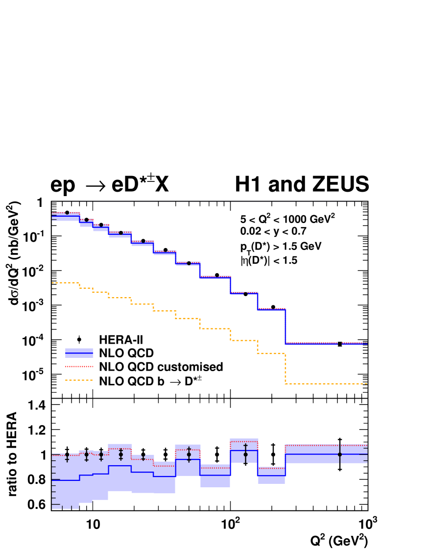
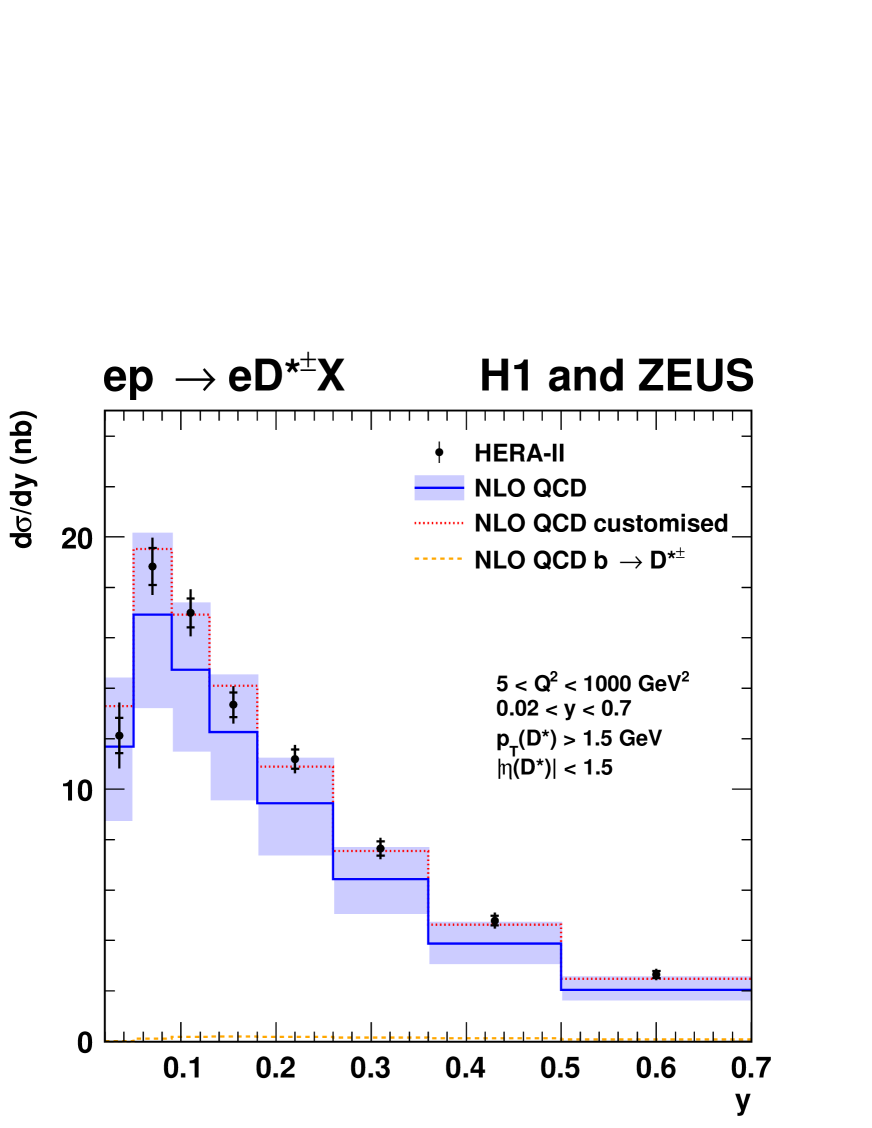
in Figures 6 – 10.
In general, the predictions describe the data well. The data reach an
overall precision of about 5% over a large fraction of the measured
phase space,
while the typical theoretical uncertainty ranges from 30% at low to 10%
at high . The data points in the different distributions are
statistically and systematically correlated. No attempt is made
in this paper to quantify the correlations between bins taken from two
different distributions.
Thus quantitative comparisons of theory to data can only be made for individual distributions.
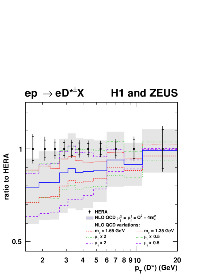
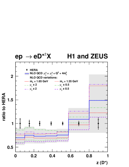
In order to study the impact of the current theoretical uncertainties in more detail, the effect of some variations on the predictions is shown separately in Figure 11, compared to the same data as in Figures 6, 8 and 10. Only the variations with the largest impact on the respective distribution are shown in each case.
-
1.
The NLO prediction as a function of (Figure 11, top) describes the data better by either
-
•
setting the charm-quark pole mass to 1.35 GeV or
-
•
reducing the renormalisation scale by a factor 2 or
-
•
increasing the factorisation scale by a factor 2.
Simultaneous variation of both scales in the same direction would largely compensate and would therefore have a much smaller effect.
-
•
- 2.
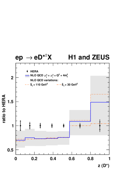
-
3.
The preference for a reduced renormalisation scale already observed for is confirmed by the distribution (Figure 11, bottom right). However, the shape of the distribution rather prefers variations of the charm mass and the factorisation scale in the opposite direction to those found for the distribution. The distributions of the other kinematic variables do not provide additional information to these findings [52].
As stated before, within the large uncertainties indicated by the theory bands in Figures 1 – 5, all distributions are reasonably well described. However, the above study shows that the different contributions to these uncertainties do not only affect the normalisation, but also change the shape of different distributions in different ways. It is therefore not obvious that a variant of the prediction that gives a good description of the distribution in one variable will also give a good description of the distribution in another.
Based on the study if items 1.-3. above, a ‘customised’ calculation is performed to demonstrate the possibility of obtaining an improved description of the data in all variables at the same time, both in shape and normalisation, within the theoretical uncertainties quoted in Section 2. For this calculation, the following choices were made:
-
•
From the three options discussed in item 1. above, the second is chosen, i.e. the renormalisation scale is reduced by a factor 2, with the factorisation scale unchanged.
-
•
The change of the fragmentation parameter GeV2, as discussed in item 2. above, is applied.
-
•
At this stage, the resulting distributions are still found to underestimate the data normalisation. As the renormalisation and factorisation scales are recommended to differ by at most a factor of two [53], the only significant remaining handle arising from items 1. and 3. is the charm-quark pole mass. This mass is set to 1.4 GeV, a value which is also compatible with the partially overlapping data used for a previous dedicated study [21] of the charm-quark mass.
- •
The result of this customised calculation is indicated as a dotted line in Figures 6 – 10. A reasonable agreement with data is achieved simultaneously in all variables. This a posteriori adjustment of theory parameters is not a prediction, but it can be taken as a hint in which direction theoretical and phenomenological developments could proceed. The strong improvement of the description of the data relative to the central prediction through the customisation of the renormalisation scale is in line with the expectation that higher-order calculations will be helpful to obtain a more stringent statement concerning the agreement of perturbative QCD predictions with the data. The improvement from the customisation of one of the fragmentation parameters and the still not fully satisfactory description of the distribution indicate that further dedicated experimental and theoretical studies of the fragmentation treatment might be helpful.
In general, the precise single-differential distributions resulting from this combination, in particular those as a function of , and , are sensitive to theoretical and phenomenological parameters in a way which complements the sensitivity of more inclusive variables like and .
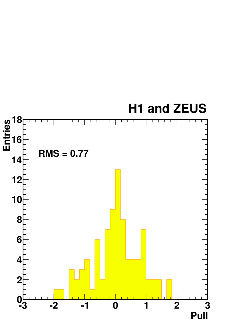
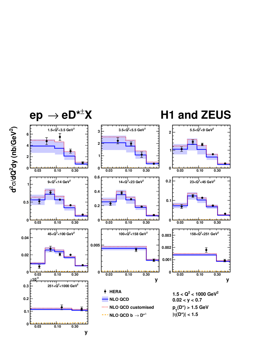
The combined double-differential cross sections with the uncorrelated, correlated and total uncertainties666A detailed breakdown of correlated uncertainties can be found on http://www.desy.de/h1zeus/dstar2015/. as a function of and are given in Table 9. The total uncertainty is obtained by adding the uncorrelated and correlated uncertainties in quadrature. The individual data sets as well as the results of the combination are shown in Figure 12. Including data set IV slightly reduces the overall cross-section normalisation with respect to the combination of sets I–III only. The pull distribution of the combination is shown in Figure 13. The combination has a probability of 84%, i.e. all data sets are consistent. The shifts and reductions of the correlated uncertainties are given in Table 8.
These combined cross sections are compared to NLO predictions777The NLO QCD prediction for the beauty contribution to production,
calculated as described in Section 2, can be found on
http://www.desy.de/h1zeus/dstar2015/. in Figure 14.
The customised calculation is also shown.
In general the predictions describe the data well. The data have a
precision of about 5–10% over a large fraction of the measured phase space,
while the estimated theoretical uncertainty ranges from 30% at low to 10%
at high .
As well as the single-differential distributions, these double-differential distributions
give extra input to test further theory improvements.
6 Conclusions
Measurements of -production cross sections in deep-inelastic scattering by the H1 and ZEUS experiments are combined at the level of visible cross sections, accounting for their systematic correlations. The data sets were found to be consistent and the combined data have significantly reduced uncertainties. In contrast to the earlier charm combination at the level of reduced cross sections, the present combination does not have significant theory-related uncertainties and in addition distributions of kinematic variables of the mesons are obtained. The combined data are compared to NLO QCD predictions. The predictions describe the data well within their uncertainties. Higher order calculations would be helpful to reduce the theory uncertainty to a level more comparable with the data precision. Further improvements in the treatment of heavy-quark fragmentation would also be desirable.
Acknowledgements
We are grateful to the HERA machine group whose outstanding efforts have made these experiments possible. We appreciate the contributions to the construction, maintenance and operation of the H1 and ZEUS detectors of many people who are not listed as authors. We thank our funding agencies for financial support, the DESY technical staff for continuous assistance and the DESY directorate for their support and for the hospitality they extended to the non-DESY members of the collaborations. We would like to give credit to all partners contributing to the EGI computing infrastructure for their support.
References
- [1] C. Adloff et al. [H1 Collaboration], Z. Phys C72, (1996) 593 [hep-ex/9607012].
- [2] J. Breitweg et al. [ZEUS Collaboration], Phys. Lett. B407, (1997) 402 [hep-ex/9706009].
- [3] C. Adloff et al. [H1 Collaboration], Nucl. Phys. B545, (1999) 21 [hep-ex/9812023].
- [4] J. Breitweg et al. [ZEUS Collaboration], Eur. Phys. J. C12, (2000) 35 [hep-ex/9908012].
- [5] C. Adloff et al. [H1 Collaboration], Phys. Lett. B528, (2002) 199 [hep-ex/0108039].
- [6] S. Chekanov et al. [ZEUS Collaboration], Phys. Rev. D69, (2004) 012004 [hep-ex/0308068].
- [7] A. Aktas et al. [H1 Collaboration], Eur. Phys. J. C38, (2005) 447 [hep-ex/0408149].
- [8] A. Aktas et al. [H1 Collaboration], Eur. Phys. J. C40, (2005) 349 [hep-ex/0411046].
- [9] A. Aktas et al. [H1 Collaboration], Eur. Phys. J. C45, (2006) 23 [hep-ex/0507081].
- [10] A. Aktas et al. [H1 Collaboration], Eur. Phys. J. C51, (2007) 271 [hep-ex/0701023].
- [11] S. Chekanov et al. [ZEUS Collaboration], JHEP 07, (2007) 074 [arXiv:0704.3562].
- [12] S. Chekanov et al. [ZEUS Collaboration], Eur. Phys. J. C63, (2009) 171 [arXiv:0812.3775].
- [13] S. Chekanov et al. [ZEUS Collaboration], Eur. Phys. J. C65, (2010) 65 [arXiv:0904.3487].
- [14] F. D. Aaron et al. [H1 Collaboration], Eur. Phys. J. C65, (2010) 89 [arXiv:0907.2643].
- [15] F. D. Aaron et al. [H1 Collaboration], Phys. Lett. B686, (2010) 91 [arXiv:0911.3989].
- [16] H. Abramowicz et al. [ZEUS Collaboration], JHEP 11, (2010) 009 [arXiv:1007.1945].
- [17] F. D. Aaron et al. [H1 Collaboration], Eur. Phys. J. C71, (2011) 1509 [arXiv:1008.1731].
- [18] F. D. Aaron et al. [H1 Collaboration], Eur. Phys. J. C71, (2011) 1769 [arXiv:1106.1028].
- [19] H. Abramowicz et al. [ZEUS Collaboration], JHEP 05, (2013) 023 [arXiv:1302.5058].
- [20] H. Abramowicz et al. [ZEUS Collaboration], JHEP 05, (2013) 097 [arXiv:1303.6578]. Erratum-ibid JHEP 02, (2014) 106.
- [21] F. D. Aaron et al. [H1 and ZEUS Collaborations], Eur. Phys. J. C73, (2013) 2311 [arXiv:1211.1182].
- [22] A. Glazov, Proceedings of “13th International Workshop on Deep Inelastic Scattering”, eds. W. H. Smith and S. R. Dasu, Madison, USA, 2005, AIP Conf. Proc. 792, (2005) 237.
- [23] A. Atkas et al. [H1 Collaboration], Eur. Phys. J. C63, (2009) 625 [arXiv:0904.0929].
- [24] F. D. Aaron et al. [H1 and ZEUS Collaboration], JHEP 01, (2010) 109 [arXiv:0911.0884].
-
[25]
E. Laenen et al.,
Phys. Lett. B291, (1992) 325;
E. Laenen et al., Nucl. Phys. B392, (1993) 162;
E. Laenen et al., Nucl. Phys. B392, (1993) 229;
S. Riemersma, J. Smith and W. L. van Neerven, Phys. Lett. B347, (1995) 143 [hep-ph/9411431]. - [26] B. W. Harris and J. Smith, Phys. Rev. D57, (1998) 2806 [hep-ph/9706334].
- [27] HERAFitter-0.2.1, http://projects.hepforge.org/herafitter.
- [28] S. Alekhin, J. Blumlein and S. Moch, Phys. Rev. D86, (2012) 054009 [arXiv:1202.2281].
- [29] A. D. Martin et al., Eur. Phys. J. C70, (2010) 51 [arXiv:1007.2624].
- [30] V. G. Kartvelishvili, A. K. Likhoded and V. A. Petrov, Phys. Lett. B78, (1978) 615.
- [31] E. Lohrmann, “A summary of charm hadron production fractions”, [arXiv:1112.3757].
- [32] D. J. Lange, Nucl. Instrum. Meth. A462, (2001) 152.
- [33] C. Peterson et al., Phys. Rev. D27, (1983) 10.
- [34] H. Abramowicz et al. [ZEUS Collaboration] Eur. Phys. J. C71, (2011) 1573 [arXiv:1101.3692 ].
- [35] K. A. Olive et al. [Particle Data Group Collaboration], Chin. Phys. C38, (2014) 090001.
- [36] I. Abt et al. [H1 Collaboration], Nucl. Instrum. Meth. A386, (1997) 310.
- [37] I. Abt et al. [H1 Collaboration], Nucl. Instrum. Meth. A386, (1997) 348.
- [38] R. D. Appuhn et al. [H1 SPACAL Group], Nucl. Instrum. Meth. A386, (1997) 397.
- [39] U. Holm (ed.) [ZEUS Collaboration], “The ZEUS Detector”. Status Report (unpublished), DESY (1993), available on http://www-zeus.desy.de/bluebook/bluebook.html.
-
[40]
N. Harnew et al.,
Nucl. Instrum. Meth. A279, (1989) 290;
B. Foster et al., Nucl. Phys. Proc. Suppl. 32, (1993) 181;
B. Foster et al. [ZEUS Collaboration], Nucl. Instrum. Meth. A338, (1994) 254. - [41] J. Kretzschmar, A precision measurement of the proton structure function with the H1 experiment, PhD thesis, Humboldt University, Berlin, 2008. Also available at http://www-h1.desy.de/publications/theses_list.html.
- [42] D. Pitzl et al., Nucl. Instrum. Meth. A454, (2000) 334 [hep-ex/0002044].
- [43] I. Glushkov, D* meson production in deep inelastic electron-proton scattering with the forward and backward silicon trackers of the H1 experiment at HERA, PhD thesis, Humboldt University, Berlin, 2008. Also available at http://www-h1.desy.de/publications/theses_list.html.
- [44] A. Polini et al., Nucl. Instrum. Meth. A581, (2007) 656.
- [45] B. Andrieu et al. [H1 Calorimeter Group], Nucl. Instrum. Meth. A336, (1993) 460.
-
[46]
M. Derrick et al.,
Nucl. Instrum. Meth. A309, (1991) 77;
A. Andresen et al.[ZEUS Calorimeter Group and ZEUS Collaborations], Nucl. Instrum. Meth. A309, (1991) 101;
A. Caldwell et al., Nucl. Instrum. Meth. A321, (1992) 356;
A. Bernstein et al.[ZEUS Barrel Calorimeter Group Collaboration], Nucl. Instrum. Meth. A336, (1993) 23. - [47] B. Andrieu et al. [H1 Calorimeter Group], Nucl. Instrum. Meth. A336, (1993) 499.
- [48] T. Nicholls et al. [H1 SpaCal Group], Nucl. Instrum. Meth. A374, (1996) 149.
- [49] L. Adamczyk et al., Nucl. Instrum. Meth. A744, (2014) 80 [arXiv:1306.1391].
- [50] “The HERA luminosity upgrade”, U. Schneekloth (ed.) (DESY), July 1998, DESY-HERA-98-05.
- [51] HERAverager-0.0.1, https://wiki-zeuthen.desy.de/HERAverager.
- [52] O. Zenaiev, Charm Production and QCD Analysis at HERA and LHC, PhD thesis, Hamburg University, Hamburg, 2015.
- [53] O. Behnke et al., Benchmark cross sections for heavy flavour production, in J. Baines et al., Heavy Quarks (Working group 3), Summary report for the HERA-LHC workshop proceedings, [hep-ph/0601164].
| ( GeV) | (nb/ GeV) | |||
| : | ||||
| : | ||||
| : | ||||
| : | ||||
| : | ||||
| : | ||||
| : | ||||
| : | ||||
| : | ||||
| : | ||||
| : |
| (nb) | ||||
| : | ||||
| : | ||||
| : | ||||
| : | ||||
| : | ||||
| : | ||||
| : | ||||
| : | ||||
| : | ||||
| : | ||||
| : | ||||
| : |
| (nb) | ||||
| : | ||||
| : | ||||
| : | ||||
| : | ||||
| : | ||||
| : | ||||
| : |
| ( GeV2) | (nb/ GeV2) | |||
| : | ||||
| : | ||||
| : | ||||
| : | ||||
| : | ||||
| : | ||||
| : | ||||
| : | ||||
| : | ||||
| : | ||||
| : |
| (nb) | ||||
| : | ||||
| : | ||||
| : | ||||
| : | ||||
| : | ||||
| : | ||||
| : | ||||
| : |
| Data set | Name | ||||||||||||
|---|---|---|---|---|---|---|---|---|---|---|---|---|---|
| sh | red | sh | red | sh | red | sh | red | sh | red | sh | red | ||
| I,II | H1 CJC efficiency | ||||||||||||
| I,II | H1 luminosity | ||||||||||||
| I,II | H1 MC PDF | ||||||||||||
| I,II | H1 electron energy | ||||||||||||
| I,II | H1 electron polar angle | ||||||||||||
| I,II | H1 hadronic energy scale | ||||||||||||
| II | H1 fragmentation threshold at high | ||||||||||||
| I,II | H1 alternative MC model | ||||||||||||
| I,II | H1 alternative MC fragmentation | ||||||||||||
| I,II | H1 fragmentation threshold | ||||||||||||
| I | H1 high uncertainty | ||||||||||||
| III | ZEUS hadronic energy scale | ||||||||||||
| III | ZEUS electron energy scale | ||||||||||||
| III | ZEUS correction | ||||||||||||
| III | ZEUS window variation | ||||||||||||
| III | ZEUS tracking efficiency | ||||||||||||
| III | ZEUS MC normalisation | ||||||||||||
| III | ZEUS PHP MC normalisation | ||||||||||||
| III | ZEUS diffractive MC normalisation | ||||||||||||
| III | ZEUS MC reweighting ( and ) | ||||||||||||
| III | ZEUS MC reweighting () | ||||||||||||
| III | ZEUS luminosity (HERA-II) | ||||||||||||
| IV | ZEUS luminosity (98-00) | ||||||||||||
| I-IV | Theory variation | ||||||||||||
| I-IV | Theory , variation | ||||||||||||
| I-IV | Theory variation | ||||||||||||
| I-IV | Theory longitudunal frag. variation | ||||||||||||
| I-IV | Theory transverse frag. variation | ||||||||||||
| ( GeV2) | (nb/ GeV2) | ||||
| : | : | ||||
| : | |||||
| : | |||||
| : | |||||
| : | : | ||||
| : | |||||
| : | |||||
| : | |||||
| : | : | ||||
| : | |||||
| : | |||||
| : | |||||
| : | |||||
| : | : | ||||
| : | |||||
| : | |||||
| : | |||||
| : | |||||
| : | : | ||||
| : | |||||
| : | |||||
| : | |||||
| : | |||||
| : | : | ||||
| : | |||||
| : | |||||
| : | |||||
| : | |||||
| : | : | ||||
| : | |||||
| : | |||||
| : | |||||
| : | |||||
| : | : | ||||
| : | |||||
| : | : | ||||
| : | |||||
| : | : | ||||
| : |