Radial Velocity Curves of Ellipsoidal Red Giant Binaries in the Large Magellanic Cloud

Abstract

Ellipsoidal red giant binaries are close binary systems where an unseen, relatively close companion distorts the red giant, leading to light variations as the red giant moves around its orbit. These binaries are likely to be the immediate evolutionary precursors of close binary planetary nebula and post-asymptotic giant branch and post-red giant branch stars. Due to the MACHO and OGLE photometric monitoring projects, the light variability nature of these ellipsoidal variables has been well studied. However, due to the lack of radial velocity curves, the nature of their masses, separations, and other orbital details has so far remained largely unknown. In order to improve this situation, we have carried out spectral monitoring observations of a large sample of 80 ellipsoidal variables in the Large Magellanic Cloud and we have derived radial velocity curves. At least 12 radial velocity points with good quality were obtained for most of the ellipsoidal variables. The radial velocity data are provided with this paper. Combining the photometric and radial velocity data, we present some statistical results related to the binary properties of these ellipsoidal variables.

1. Introduction

The variable red giants in the Large Magellanic Cloud (LMC) fall on six or more distinct sequences in a period–luminosity (PL) diagram, i.e., $K$–log$P$ diagram (Wood et al., 1999; Ita et al., 2004; Soszynski et al., 2007; Fraser, Hawley, & Cook, 2008). One of these sequences, sequence E, consists of binary systems that are mainly red giant ellipsoidal binaries (Wood et al., 1999; Soszyński et al., 2004). In these ellipsoidal binary systems, the red giant is the primary and it substantially fills its Roche lobe. The secondary, which is usually an unevolved main-sequence star, is unseen observationally in most cases. Due to the substantial filling of the Roche lobe, the red giant is distorted. Rotation of the distorted shape of the red giant as the binary progresses around its orbit causes a change in the apparent light seen by a distant observer. This leads to the characteristic light and velocity curves of ellipsoidal variables that have two cycles of light variation in one orbital period but only one cycle of radial velocity variation (e.g. Nicholls et al., 2010)

The sequence E stars are low-mass stars ($m<$ 1.85 $\rm M_{\odot}$) or intermediate-mass stars (1.85 $\rm M_{\odot}$$<m<$ 7.0 $\rm M_{\odot}$). They can lie on either the red giant branch (RGB) or the asymptotic giant branch (AGB) and they are therefore in an evolutionary phase where the stellar radius is increasing. It is when the radius of the expanding red giant becomes a significant fraction of the binary separation that the ellipsoidal variability becomes detectable with current surveys such as MACHO and OGLE. The orbital periods of sequence E stars in the LMC lie in the range $\sim$30–1000 days and the light amplitude is usually $<$0.3 mag in the MACHO red band $M_{R}$. Statistically, the sequence E stars make up approximately 0.5–2% of the RGB and AGB stars in the LMC. About 7% of the sequence E stars are eclipsing and about 10% of them have unusually shaped light curves which indicate significant eccentricity of the system orbits (Soszyński et al., 2004).

Due to the MACHO and OGLE projects, the variability nature of sequence E stars is well studied. However, at the present time, there are few radial velocity studies of the sequence E stars, due to the difficulties of long-time spectral monitoring. Adams, Wood, & Cioni (2006) observed two sequence E stars in the LMC, and their preliminary results indicated that the red giant is filling its Roche lobe and transferring mass to the companion since the derived mass of the red giant is close to that of the red giant core. Nicholls et al. (2010) carried out spectral observations on 11 sequence E stars (including the two in Adams, Wood, & Cioni, 2006) to derive radial velocity variations. The average full velocity amplitude derived for those 11 sequence E samples was 43.4 km s^-1, consistent with the inference that sequence E stars are red giants in binary systems with roughly solar-mass components.

A problem with the current understanding of sequence E stars is that the eccentricity should be close to zero due to tidal interaction with the companion, yet about 10% of them have significant eccentricities (Soszyński et al., 2004). Complete orbital solutions for ellipsoidal red giant binaries with a range of eccentricities could possibly show in which part of parameter space eccentricity can be maintained. As a start to such a study, Nicholls & Wood (2012) monitored the radial velocities of 7 eccentric sequence E stars and derived complete orbital solutions.

In general, a knowledge of the complete set of orbital properties (masses, separations, eccentricities, orientations) for a large sample of ellipsoidal red giant binaries in the LMC will provide a good resource for understanding the evolution of these close binary systems. These observed parameters can be used to constrain Monte Carlo simulations of the population of sequence E stars, such as those in Nie, Wood, & Nicholls (2012). These Monte Carlo calculations provide estimates for the production rate of binary post-AGB stars, binary planetary nebulae (PNe), binary post-RGB stars, and luminous white dwarfs relative to the production rate of single-star post-AGB stars and PNe. The relative numbers of the various types of objects listed above, now quite well known in the LMC, can be used to parameterize the binary interaction process, especially common envelope evolution, and to calibrate models for the formation of cataclysmic variable stars, AM CVn systems, the progenitors of SNe Ia, etc. So knowledge of the parameters of a large sample of the precursor binaries should help us better understand the interaction processes and the evolutionary fates of close red giant binaries.

In this study, we present the results of radial velocity monitoring of a large sample of ellipsoidal variables in the LMC. In Section 2, the design of our observing project and the data reduction is described. In Section 3, we present observed properties of binary stars based on the radial velocity and light variation data. Some statistical analyses are also provided and compared with theoretical models.

2. Observations and Data Reduction

2.1. Selection of Objects

We initially selected 86 sequence E candidates from those given in Soszyński et al. (2004). Only objects with $I<16.5$ mag were considered since good radial velocities could not be obtained in a reasonable time (20 minute exposure) for fainter objects. Also, the data quality of fainter stars is relatively poor in the MACHO and OGLE databases, so their light curves have large dispersions and this is not good for fitting orbital solution.

All the sequence E candidates in Soszyński et al. (2004) and our 86 ellipsoidal variable candidates are plotted in the $I$–$\log P$ and $W$–$\log P$ planes in Figure 1, where $W=I-1.55(V-I)$ is a reddening-free Weisenheit index (Madore, 1982). It should also be noted that $P$ is the orbital period, which is twice the period obtained by Fourier analysis of raw light curves since ellipsoidal variables have two maxima and two minima of the light curve per orbital period. The sequence E variables are often plotted in PL diagrams using the semi-period.

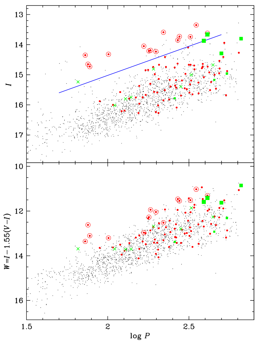
Figure 1.— Location of our 86 ellipsoidal variable candidates (red dots) on the $I$–$\log P$ and $W$–$\log P$ planes. The small black dots show the full sample of ellipsoidal variables in Soszyński et al. (2004). The blue line in the top panel is a line parallel to the main part of sequence E. Stars above this line are brighter than normal for their period and are expected to be intermediate-mass stars. Objects in our sample that lie above the line are shown in both plots as circled points. The green squares are ellipsoidal variables studied by Nicholls & Wood (2012) and the area of the square is proportional to the mass of the red giant derived by them. The green crosses are ellipsoidal variables studied by Nicholls et al. (2010). Due to the lack of $V$ band data, 3 objects of Nicholls et al. (2010) are absent.

Our aim was to select a sample of objects with as wide a set of parameters as possible. We therefore selected objects randomly throughout sequence E, as shown in Figure 1, subject to the constraint $I<16.5$. Note that the magnitude cut of 16.5 is about 2 mag below the RGB tip, so our sample includes low-mass sequence E stars, even down to the masses of globular cluster red giants. We also made no attempt to select highly eccentric stars so the sample should include a range of eccentricities (note that Nicholls & Wood, 2012, have already studied a sample of 7 eccentric sequence E stars).

At a given orbital period, more massive binary systems will have larger separations so the red giant will need to get to a higher luminosity (radius) before the Roche lobe filling factor is large enough to produce detectable ellipsoidal light variations. The more massive binaries should therefore preferentially lie in the high-luminosity side of sequence E in Figure 1. The results of Nicholls & Wood (2012), shown in Figure 1, indicate that the higher-mass stars do indeed lie on the high-luminosity side of sequence E. In order to be sure of selecting a good sample of intermediate-mass stars ($M>$$\sim$1.85 M_⊙), we preferentially included extra stars above the blue line in Figure 1. Our final sample consists of 86 stars.

With 86 ellipsoidal candidates, plus 11 sequence E stars whose radial velocities were obtained by Nicholls et al. (2010) (green crosses in Figure 1) and the 7 eccentric sequence E stars studied by Nicholls & Wood (2012) (green squares in Figure 1) , we have a combined sample of approximately 100. The full sample will give us statistical information about properties such as masses, mass ratio, eccentricity, separation, Roche lobe filling factor, and red giant luminosity for field red giants in the LMC. Derivation of some of these properties will require the use of a binary orbit modeling tool such as the Wilson–Devinney code (Wilson & Devinney, 1971; Wilson, 1979, 1990; Wilson et al., 2009).

2.2. Spectral Observation

The radial velocity observations were taken using the Wide Field Spectrograph (WiFeS; Dopita et al., 2007, 2010) mounted on the Australian National University 2.3m telescope at Siding Spring Observatory. WiFes is an integral field, double-beam, imaging-slicing spectrograph with a field of view 25$\times$38 square arcsec, imaged onto 25 slits that are 1 arcsec wide and 38 arcsec long. It has six gratings, giving high (R=7000) and low (R=3000) spectral resolutions. For our observations, the gratings B7000 (wavelength coverage of 4184–5580Å) and I7000 (wavelength coverage of 6832–9120Å) were chosen for the blue and red CCD, respectively. These two gratings give a two-pixel resolution R=7000, corresponding to a 45 km s^-1 velocity resolution.

We carried out 18 weeks of radial velocity monitoring, from 2010 September to 2012 March, to cover at least one orbital period for nearly all of the 86 objects. The observations were approximately evenly distributed throughout the 18 months, roughly one radial velocity observation per star per month. The exposure time was generally set to 300 s for objects with $I$$\sim$13 mag, 600 s for $I$$\sim$14 mag, and 900 s for $I$$\sim$15 mag, which gives a signal-to-noise ratio (S/N) of at least 20. For fainter objects ($I>$16 mag), the exposure time was increased to 1200 s. We also increased the exposure time when observing in bad weather, to guarantee a S/N of 20.

For our observations, we chose the “stellar” mode exposure, in which case only 12 slits of the spectrograph were used. For flatfielding the QI-1 lamp was used and for wavelength calibration a Ne–Ar arc lamp exposure was taken at the beginning of the night. For velocity derivation, the radial velocity standard star HR9014 was observed. In addition, the white dwarf star EG131 was observed so that telluric lines could be used to remove any zero point error in the wavelength calibration arising from spectrograph drift over the night. To achieve high S/N, the exposure times of HR9014 and EG131 were set to 10 s and 900 s, respectively.

2.3. Data Reduction

2.3.1 Spectrum Reduction

The WiFes data reduction pipeline (Dopita et al., 2010) was used for the spectrum reduction. The pipeline combines the calibration and science data and provides one-dimensional spectra with most of the cosmic rays and sky emission lines removed. Since all our objects are red, most of their flux is concentrated in the red region of the spectrum. Therefore, we did not reduce the blue beam spectra because these spectra are of low S/N. The red spectra (6832–9120Å) contain many prominent telluric absorption lines as well as emission lines of water, OH, and O₂. The pipeline-reduced spectra sometimes contained some residual telluric lines and cosmic rays. Because of this, we checked by eye all the reduced spectra of the same object and, by comparison, removed residual cosmic rays and residual sky emission lines manually.

Spectrally, red giant binaries with white dwarf or neutron star companions always show characteristic emission lines (Allen, 1984; Kenyon, 1986; Mikolajewska et al., 1997; Belczyński et al., 2000). These objects are the symbiotic stars. In passing, we note that none of our ellipsoidal variables show emission lines in their spectra. This means that none of the companions are likely to be white dwarfs or neutron stars.

2.3.2 Radial Velocity Calculation

1. Relative radial velocity The relative radial velocity and its error were computed using the IRAF $fxcor$ package. The $fxcor$ package uses a Fourier cross-correlation method to find the wavelength shift between an object and a template spectrum in a specified cross-correlation region. The template was usually a radial velocity standard star with well-determined radial velocity and a spectral type similar to that of the program object. In our case, all the 86 ellipsoidal variables are stars of K–M spectral type, so we choose as the template HR9014, which is a K5 star with a well-determined radial velocity of $-20.4$ km s^-1. The cross correlation was made on the wavelength interval 8400–8750 Å which contains the Ca II triplet lines and is relatively free of telluric lines. The heliocentric radial velocity ($\rm{\upsilon_{helio}(obj)}$), obtained from $fxcor$ after heliocentric correction and the inclusion of the heliocentric radial velocity of HR9014, was saved along with its error. The error in $\rm{\upsilon_{helio}(obj)}$ is normally below 4 km s^-1. If the error was larger than 10 km s^-1 (due to bad weather and low S/N), then the velocity point was excluded from our data set.

2. Zero-point correction To check the velocity calibration, all spectra of each program star were cross correlated with a template consisting of a single spectrum of the telluric standard star EG131. EG131 is a white dwarf that radiates almost like a blackbody. Thus, its spectrum has only telluric lines, making it an ideal template for the zero-point correction. In principle, the relative velocity of the telluric lines in different spectra should be zero, but, due to the movement of the CCD system and spectrograph between the taking of the arc spectrum at the beginning of the night and the taking of the object spectrum, as well as the changes of the atmospheric pressure, there can be shifts in velocity. To compute this zero-point velocity shift $\rm{\upsilon_{zp}(obj)}$, program stars were cross correlated with EG131 in the wavelength interval of 8120–8370 Å. This region is dominated by telluric lines and it is close to the region of Ca II triplet, so the zero-point correction in this region should similar to that of Ca II triplet region. The zero-point velocity correction varied from about $-$10 to 34 km s^-1 across the many nights of the observation. HR9014 was also cross correlated with EG131 to obtain its zero point velocity correction ($\rm{\upsilon_{zp}(HR9014)}$).

3. Absolute radial velocity To compute the absolute value for the observed radial velocity $\rm{\upsilon_{r}}$ including a zero-point correction, we use the formula

   $$\rm{\upsilon_{r}=\upsilon_{helio}(obj)-\upsilon_{zp}(obj)+\upsilon_{zp}(HR9014)}~{}~{}.$$ (1)

The final radial velocity data for 2 objects are given in Table 1. The full table is available online.

Table 1Radial velocities $\rm{\upsilon_{r}}$ and 1$\sigma$ Errors $\sigma_{\rm{\upsilon_{r}}}$ in km s^-1. Stars are identified by their OGLE II R.A. and decl.

OGLE 050659.79 -692540.4			OGLE 051256.36 -684937.5
HJD( 2450000+)	$\rm{\upsilon_{r}}$	$\sigma_{\rm{\upsilon_{r}}}$	HJD( 2450000+)	$\rm{\upsilon_{r}}$	$\sigma_{\rm{\upsilon_{r}}}$
5463.06104	246.14	1.74	5461.14209	237.26	1.70
5513.99023	251.84	2.10	5513.03125	247.21	1.64
5563.00781	284.43	1.48	5563.07324	257.77	1.54
5590.98877	270.53	2.71	5590.06592	256.17	2.27
5603.96924	257.47	2.12	5647.92578	243.94	1.51
5649.00684	232.40	1.40	5673.95508	229.63	2.68
5678.97363	264.23	4.53	5693.92676	230.36	1.53
5679.01221	250.28	4.04	5765.23242	231.89	2.03
5764.26514	246.01	3.65	5846.08301	242.70	1.92
5783.19287	239.24	1.88	5867.01807	252.29	1.39
5848.15039	273.73	7.73	5907.19336	257.03	1.75
5868.03613	282.79	2.54	5944.04883	255.03	1.35
5906.11133	270.63	1.82	5991.98584	243.43	1.50
5944.17676	242.22	3.00	-	-	-

3. Results

3.1. Properties of the Observed Ellipsoidal Variables

Before presenting the properties of the observed ellipsoidal variables, we need to remove candidates that are not clearly ellipsoidal variables with the help of the observed radial velocity. Among our 86 objects, we found that 80 of them are real ellipsoidal variables, showing two light maxima and two minima but only one velocity maximum and minimum in one orbital period. The remaining 6 candidates do not clearly satisfy this requirement due to their low-velocity amplitude relative to the noise so they were removed. These 6 objects could be ellipsoidal variables whose orbital plane lies close to the plane of the sky or they could be sequence D stars as these stars lie close to the sequence E stars in the $I$–$\log P$ and $W$–$\log P$ planes and they have small velocity amplitudes (Nicholls et al., 2009). For the remainder of this paper, we focus on the 80 real ellipsoidal variables while we discuss the 6 rejected objects in the Appendix.

Table 2 shows various properties of the 80 ellipsoidal variables. For all objects, the period given has been re-derived because the original value from Soszyński et al. (2004) is not accurate enough. The MACHO and OGLE II light curve data were taken more than 10 years before our radial velocity data, which was obtained between years 2010 and 2012. Because of the long time span between the two sets of data, a small error in the period can cause a significant error in the phase of the light curve projected forward by more than 10 years. To obtain a more reliable period, when OGLE III data existed, we combined OGLE III and OGLE II light curves (covering the interval 1998–2009) and used the phase dispersion minimization (PDM) method (Stellingwerf, 1978) to calculate the period from the combined light curve. If the OGLE III data was not available for an object, we combined the OGLE II and MACHO data, covering the interval 1992–2000.

The effective temperature was calculated by converting $(I-K)_{0}$ to $T_{\rm eff}$ using spline fits to the data in Houdashelt et al. (2000a, b). The reason we used $(I-K)_{0}$ as the color index is because most of our sequence E stars are K- or early-M-type stars, and for these red giants $I-K$ varies much more with $T_{\rm eff}$ than $J-K$ so that photometric errors are less important for $I-K$. The mean $I$ magnitude was derived from the OGLE photometry, while the $K$ magnitude was obtained from the Two Micron All Sky Survey (2MASS) catalog (Cutri et al., 2003) . To remove reddening, we adopted $E(B-V)$=0.08 (Keller & Wood, 2006) along with $E(V-I)=1.38~{}\times E(B-V)$ (Schlegel, Finkbeiner, & Davis, 1998), and $E(V-K)=2.744~{}\times E(B-V)$ and $A(K)=0.35~{}\times E(B-V)$ (Rieke & Lebofsky, 1985). The bolometric correction BC_K was calculated from $(I-K)_{0}$ using the data in Houdashelt et al. (2000a, b) and the bolometric luminosity was calculated from $K_{\rm 0}$ and BC_K, with a distant modulus of the LMC 18.54 (Keller & Wood, 2006).

Finally, in Table 2, we indicate whether a star is below (a “1” in the last column) or above (a “2” in the last column) the higher-mass line in Figure 1. The last column in Table 2 also provides notes on unusual variability characteristics as given in Soszyński et al. (2004). Stars for which there is OGLE III data available are also indicated. The data in Table 2 are available online.

Table 2Properties of the observed ellipsoidal variables

No	Object	$P$	$I$	$V$	$M_{B}$	$M_{R}$	$K$	$\Delta{I}$	$\Delta{\rm RV}$	$L$	$T_{\rm eff}$	$R$	Remark
	(OGLE II Name)	(day)	(mag)	(mag)	(mag)	(mag)	(mag)	(mag)	(km s-1)	($\rm L_{\odot}$)	(K)	($\rm R_{\odot}$)
1	050107.08–692036.9	166.8	14.05	14.75	-	-	13.14	0.110	70	3278	5773	58	2,ogle3
2	050222.40–691733.6	107.8	16.00	17.53	16.85	15.87	13.90	0.070	32	581	3990	51	1
3	050254.15–692013.8	171.5	15.67	17.08	-	-	13.82	0.025	35	736	4234	51	1
4	050258.71–684406.6	433.8	15.24	16.96	16.85	15.65	13.18	0.040	38	1149	4020	71	1
5	050334.97–685920.5	101.1	14.32	15.04	14.85	14.40	13.36	0.200	110	2526	5666	53	2
6	050350.55–691430.2	224.7	15.51	17.10	16.85	15.78	13.46	0.060	24	896	4030	62	1
7	050353.41–690230.8	323.6	14.67	16.36	16.28	15.13	12.65	0.060	7	1915	4049	90	1,ogle3
8	050438.97–693115.3	383.2	14.75	16.24	-	-	12.99	0.070	14	1673	4321	74	1
9	050454.49–690401.2	220.2	13.59	14.28	-	13.72	12.79	0.070	120	5175	6018	67	2,ogle3
10	050504.70–683340.3	238.9	15.82	17.25	16.95	16.00	14.05	0.040	40	631	4327	45	1
11	050512.19–693543.5	204.3	16.02	17.50	17.30	16.33	13.92	0.050	40	570	3988	51	1
12	050554.57–683428.5	270.1	13.85	15.39	15.10	14.07	11.85	0.035	26	4028	4061	129	2
13	050558.70–682208.9	264.0	15.43	16.88	-	-	13.48	0.020	22	938	4128	60	1
14	050604.99–681654.9	201.7	15.59	16.99	17.01	15.98	13.69	0.030	30	802	4174	55	1
15	050610.03–683153.0	318.5	15.59	17.19	-	-	13.71	0.030	35	798	4197	54	1,e
16	050651.36–695245.4	220.2	15.85	17.49	17.30	16.13	13.96	0.045	30	630	4192	48	1
17	050659.79–692540.4	156.4	15.37	16.84	16.74	15.75	13.54	0.070	50	963	4254	58	1
18	050709.66–683824.8	206.1	15.14	16.67	16.65	15.60	13.19	0.060	37	1223	4121	69	1
19	050720.82–683355.2	521.4	13.94	15.50	15.53	14.42	11.95	0.020	30	3699	4072	123	2
20	050758.17–685856.3	198.1	14.23	15.64	15.50	14.56	12.37	0.050	45	2744	4210	99	1
21	050800.52–685800.8	276.2	13.73	15.14	15.02	14.06	11.87	0.050	42	4337	4199	126	2
22	050843.38–692815.1	121.8	16.21	17.67	17.30	16.32	14.23	0.040	23	464	4098	43	1
23	050900.02–690427.2	156.5	15.96	17.42	17.25	16.23	14.14	0.025	16	561	4273	44	1
24	050948.63–690157.4	75.60	14.65	15.96	15.80	14.85	13.06	0.200	26	1779	4529	69	2
25	051009.20–690020.0	321.3	15.32	16.99	16.79	15.63	13.27	0.027	20	1067	4024	68	1,e
26	051050.92–692228.0	326.2	15.19	16.67	16.40	15.47	13.39	0.035	14	1128	4284	62	1,ogle3
27	051101.04–691425.1	282.5	15.69	17.15	16.95	15.97	13.78	0.030	20	732	4173	52	1,e
28	051200.23–690838.4	641.3	14.27	16.34	16.13	14.80	11.89	0.030	14	3131	3737	135	1,e+sr,ogle3
29	051205.44–684559.9	390.5	15.08	16.62	16.57	15.54	12.90	0.060	27	1382	3912	82	1,ogle3
30	051220.63–684957.8	486.5	14.54	16.27	16.10	14.92	12.45	0.070	19	2202	3983	99	1,e+sr,ogle3
31	051256.36–684937.5	341.9	14.82	16.82	16.60	15.28	12.50	0.130	29	1851	3784	101	1,ogle3
32	051345.17–692212.1	197.9	16.24	17.74	17.50	16.38	14.19	0.040	42	459	4038	44	1
33	051347.73–693049.7	306.6	15.48	17.09	-	-	13.52	0.040	20	899	4114	60	1,e
34	051515.95–685958.1	322.7	13.74	15.18	15.02	13.98	11.91	0.030	24	4269	4229	123	2,e
35	051620.47–690755.3	240.7	15.17	16.94	16.85	15.58	13.05	0.150	40	1249	3963	76	1,ogle3
36	051621.07–692929.6	179.3	14.21	15.46	15.17	14.36	12.43	0.030	17	2748	4294	96	2
37	051653.08–690651.2	269.2	14.63	16.36	16.35	14.93	12.32	0.080	29	2193	3792	110	1
38	051738.19–694848.4	297.7	15.45	17.03	16.80	15.73	13.31	0.050	29	975	3943	68	1,e
39	051746.55–691750.2	225.2	14.41	16.01	-	-	12.33	0.050	15	2478	3985	105	1
40	051818.84–690751.3	463.9	15.46	17.29	-	-	13.03	0.050	26	1076	3710	80	1,e
41	051845.02–691610.5	320.0	15.65	16.97	-	-	13.90	0.040	55	734	4349	48	1
42	052012.26–694417.5	177.4	14.84	16.46	-	15.23	12.75	0.040	18	1675	3983	87	1
43	052029.90–695934.1	171.0	14.85	16.05	15.88	15.00	13.23	0.045	50	1489	4492	64	1
44	052032.29–694224.2	72.70	14.35	14.99	14.73	14.31	13.52	0.060	60	2569	5973	48	2,e
45	052048.62–704423.5	488.5	14.79	-	-	-	12.95	0.030	5	1641	4231	76	1
46	052115.05–693155.1	194.9	14.98	16.08	15.78	15.03	13.38	0.020	49	1318	4525	60	1
47	052117.49–693124.8	243.3	15.39	16.97	16.60	15.55	13.21	0.060	38	1044	3908	71	1
48	052119.56–710022.1	300.9	14.97	16.84	16.65	15.40	12.79	0.010	23	1531	3907	86	1,ogle3
49	052203.16–704507.8	362.5	15.62	17.01	16.72	15.82	14.04	0.035	14	734	4564	44	1
50	052228.85–694313.7	231.0	14.74	16.04	15.77	14.85	12.99	0.030	37	1684	4334	74	1
51	052238.43–691715.1	77.53	14.73	15.78	15.41	14.74	13.47	0.070	55	1638	5046	53	2
52	052324.57–692924.2	312.4	14.09	15.16	15.08	14.43	12.39	0.030	40	3016	4388	96	2
53	052422.28–692456.2	485.4	14.95	16.67	16.65	15.49	12.82	0.060	18	1535	3948	85	1,+sr,ogle3
54	052425.52–695135.2	206.7	14.67	16.04	15.87	15.03	12.93	0.040	42	1792	4345	75	1
55	052438.19–700435.9	192.8	15.57	16.96	16.70	15.87	13.79	0.040	25	794	4314	51	1
56	052438.40–700028.8	410.8	13.62	15.11	14.83	14.00	11.71	0.060	50	4852	4147	136	2,e
57	052458.88–695107.0	340.6	14.67	16.53	16.33	15.20	12.35	0.075	5	2117	3790	108	1,+sr,ogle3
58	052510.82–700123.9	189.7	14.74	16.05	15.87	15.05	12.99	0.030	30	1686	4328	74	1
59	052513.34–693025.2	259.4	14.76	16.03	15.97	15.14	13.12	0.030	45	1621	4471	68	1
60	052542.11–694847.4	514.6	14.41	16.04	15.90	14.85	12.35	0.030	35	2461	4004	104	1,e
61	052554.91–694137.4	182.8	15.30	16.87	16.95	15.85	13.23	0.120	40	1092	4008	69	1
62	052703.65–694837.7	350.4	13.35	14.85	14.70	13.78	11.43	0.100	60	6230	4131	156	2
63	052833.50–695834.6	183.2	14.19	15.64	15.65	14.75	12.31	0.060	20	2861	4186	103	2
64	052928.90–701244.2	531.5	15.68	17.29	-	-	13.71	0.060	25	751	4105	55	1,e
65	052948.84–692318.7	421.7	14.92	16.85	16.55	15.35	12.70	0.070	16	1625	3873	90	1,e+sr,ogle3
66	052954.82–700622.5	154.7	16.27	17.66	17.48	16.63	14.33	0.050	40	434	4149	41	1
67	053141.27–700647.1	384.1	14.73	16.78	-	-	12.36	0.090	24	2044	3751	108	1,e+sr,ogle3
68	053156.08–693123.0	412.2	14.73	16.50	-	-	12.57	0.070	22	1899	3916	96	1,e+sr,ogle3
69	053202.44–693209.2	426.5	15.51	17.12	-	-	13.48	0.030	25	892	4042	62	1,e
70	053219.66–695805.0	89.55	15.85	17.32	16.70	15.90	12.14	0.010	18	1749	3264	132	1
71	053226.48–700604.7	454.7	15.00	16.78	16.43	15.28	12.72	0.070	40	1547	3817	91	1,e+sr,ogle3
72	053337.07–703111.7	315.5	14.67	16.76	16.60	15.28	12.37	0.130	16	2108	3799	107	1,e,ogle3
73	053338.94–694455.2	126.9	16.19	17.75	17.60	16.51	14.23	0.090	32	469	4128	43	1
74	053356.79–701919.6	205.3	16.27	17.69	17.53	16.55	14.35	0.040	40	432	4169	40	1
75	053438.78–695634.1	384.7	14.64	16.69	16.35	15.07	12.28	0.070	19	2218	3751	113	1,ogle3
76	053733.21–695026.9	263.0	15.18	16.85	16.84	15.63	13.07	0.050	19	1235	3970	75	1
77	053946.88–704257.8	265.0	16.09	17.81	17.78	16.55	13.93	0.040	41	547	3929	51	1
78	054006.47–702820.4	361.5	15.26	16.98	16.85	15.63	13.08	0.070	29	1176	3906	76	1,e,ogle3
79	054258.34–701609.2	164.0	15.75	17.29	-	-	13.79	0.040	20	703	4114	53	1
80	054736.16–705627.2	135.9	15.79	17.31	17.05	16.03	13.96	0.030	35	657	4253	48	1

Note. — Columns 4–8 are mean magnitudes in different bands; Column 9 is the mean amplitude of light variability in $I$ band; Column 10 is the full amplitude of radial velocity; Columns 11–13 are the luminosity, effective temperature and mean radius derived as described in the text; Column 14 contains remarks: number 1 for stars below the line in Figure 1 and number 2 for stars above the line, lower case letters stand for binary types: “$e$,” eccentric, “$+sr$,” a binary whose red giant shows semi-regular variability as well as ellipsoidal variability, and “ogle3” denotes an object which has OGLE III light curve data.

3.2. Light Curves and Radial Velocity Curves

We present samples of light and radial velocity curves for the ellipsoidal variables in Figure 2. Light and radial velocity curves for all objects are available as online data. The time series data for the light curves are from the MACHO, OGLE II, and OGLE III databases if they are available. Each radial velocity curve has at least 12 good quality data points in one orbital period, good enough for a binary orbital solution. As confirmed by Nicholls et al. (2010), our observed ellipsoidal variables show two light maxima and two minima in one orbital period, while the velocity shows only one maximum and one minimum. Among our 80 objects, most of them (60/80=75%) have almost circular orbits, since they have equal light maxima and they have the same light curve widths for the first and second maxima (e.g., the top two objects of Figure 2). The other systems are eccentric binaries (20/80=25%) since they show different light maxima or light curve widths in one orbital period (e.g., the bottom two objects of Figure 2). In addition, there are binary systems that contain a semi-regular pulsating red giant (8/80=10%) (e.g., object OGLE 052948.84 in Figure 2), similar to those noted by Nicholls & Wood (2012). For these systems, both pulsation theory and binary theory can be used to constrain and compare stellar parameters.

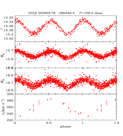
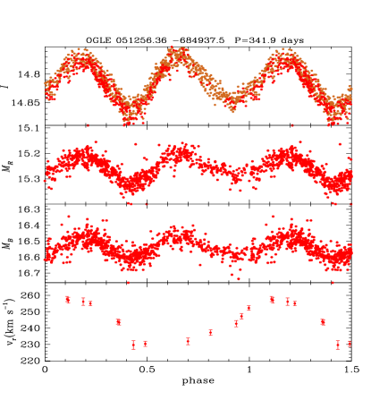
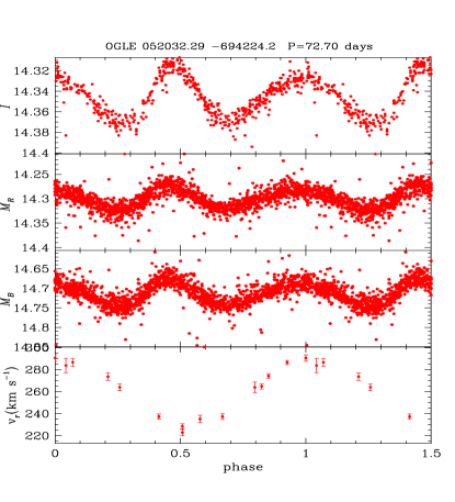
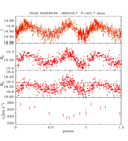
Figure 2.— Light and radial velocity curves of ellipsoidal variables. $M_{R}$ and $M_{B}$ are the MACHO red and blue magnitudes, respectively. The top two objects are ellipsoidal variables with circular orbits while the bottom two have eccentric orbits. For the $I$ band data, chocolate points are from OGLE III and red points are from OGLE II.

3.3. The Velocity Amplitude

The distribution of full radial velocity amplitude $\Delta RV$ for the 80 ellipsoidal variables plus the combined sample from Nicholls et al. (2010) and Nicholls & Wood (2012) is presented in the left panel of Figure 3 (red). From the figure, it can be seen that the velocity amplitude varies from $\sim$5 to $\sim$130 km s^-1, with a peak near 30 km s^-1. Note that the number of stars with velocity amplitudes larger than 80 km s^-1 is small.

Our observed velocity amplitude distribution is also compared to the model prediction of Nie, Wood, & Nicholls (2012) (the black dashed line in the left panel of Figure 3). The predicted distribution is for ellipsoidal red giant binaries on the top one magnitude of the RGB (870–2190 L_⊙) that have light amplitudes detectable by the OGLE II observations. Our comparison sub-sample of observations consists of 51 objects for which the luminosity lies on the top one magnitude of the RGB (the blue solid line in the left panel). Note that we compare to the model of Nie, Wood, & Nicholls (2012) which is calibrated on the OGLE II data of Soszyński et al. (2004) because that calibration is better than the one based on MACHO data due to the extra sensitivity of OGLE II observations to small-amplitude light variations.

The cumulative distributions corresponding to the histograms of the ellipsoidal variables on the top one magnitude of the RGB in Figure 3 are shown in the right panel. A two-sample Kolmogorov–Smirnov test gives a probability of up to 0.20 that the observation and model come from the same underlying distribution. There is thus a modest probability that the model is consistent with both the OGLE II photometry and the velocity amplitudes derived in this study.

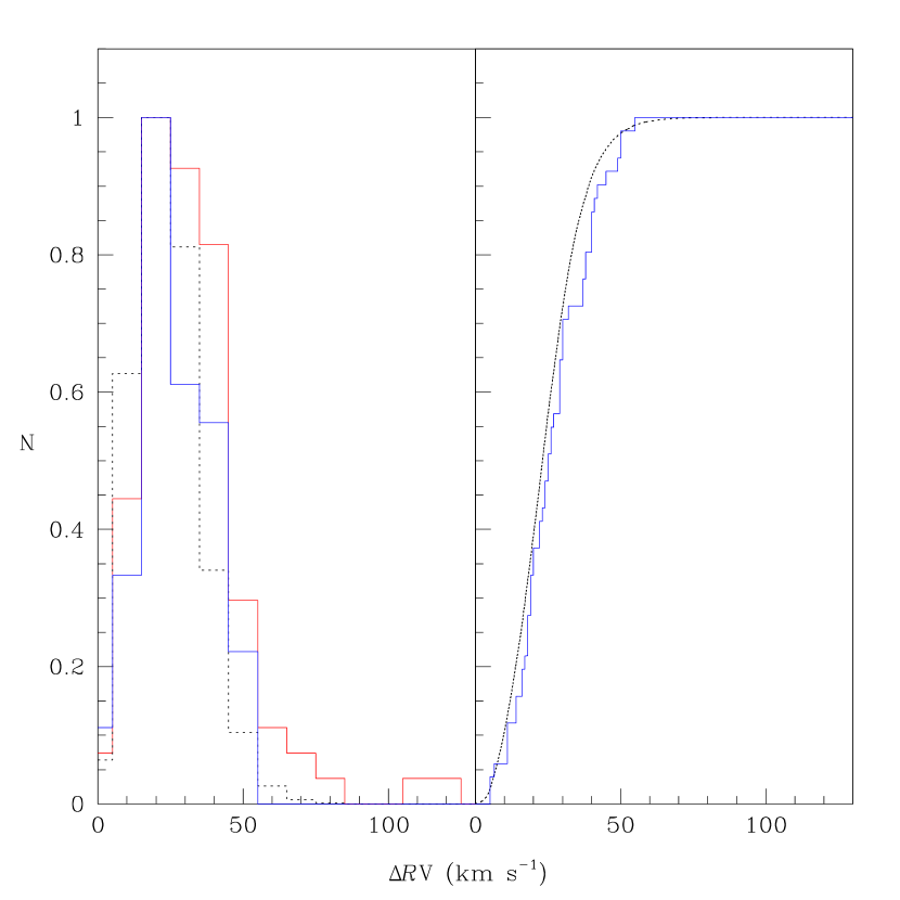
Figure 3.— Distribution of the full radial velocity amplitude $\Delta\rm RV$. Left panel: the red solid line shows the distribution for the 80 ellipsoidal variables and the combined sample of Nicholls et al. (2010) and Nicholls & Wood (2012), the blue solid line shows the observed distribution for 51 ellipsoidal variables on the top one magnitude of the RGB, and the black dashed line shows the predicted distribution for ellipsoidal variables on the top one magnitude of the RGB by the model of Nie, Wood, & Nicholls (2012) with the calibration of OGLE II data. Right panel: the predicted cumulative distribution for ellipsoidal variables on the top one magnitude of the RGB. Blue is for observations from 51 objects, and black is for the model of Nie, Wood, & Nicholls (2012) with the calibration of OGLE II data. Note that all the distribution peaks are normalized to unity.

3.4. The Mass Function

The binary mass function $f_{1}$ of a binary system where the primary star (in our case, the red giant) is observable is

$$f_{1}=\frac{K_{1}^{3}P}{2\pi~{}G}=\frac{m_{2}^{3}\sin^{3}~{}i}{(m_{1}+m_{2})^{2}}~{},$$ (2)

where $K_{1}$ is the radial velocity semi-amplitude of the primary star, $P$ is the orbital period, $m_{1}$ is the mass of the primary star, and $m_{2}$ is the mass of the secondary star. Note that $f_{1}$ is a minimum estimate for $m_{2}$. The distribution of $f_{1}$ for our sample of red giant ellipsoidal variables in the LMC is shown in Figure 4. The figure shows a peak at about 0.2 $\rm M_{\odot}$, presumably due to the dominant low-mass population, but there are a few objects that must be in more massive binaries where the secondary star is of intermediate- mass with $m_{2}\gtrsim 4~{}\rm M_{\odot}$. Red giants of this mass were found in ellipsoidal binaries in the LMC by Nicholls & Wood (2012). If we assume a random pole orientation for the binary orbit, which implies that the mean of $\sin^{3}i=\frac{3\pi}{16}$, and if we also assume that the mean mass ratio is $q=1$, then for stars in the peak of the distribution around $f_{1}\sim 0.2~{}{\rm M_{\odot}}$, the mean mass of the red giant is $m_{1}\sim$1.35 ${\rm M_{\odot}}$. This is similar to peak in the mass distribution of red giants predicted by modeling the star formation history of the LMC (e.g., Nie, Wood, & Nicholls, 2012).

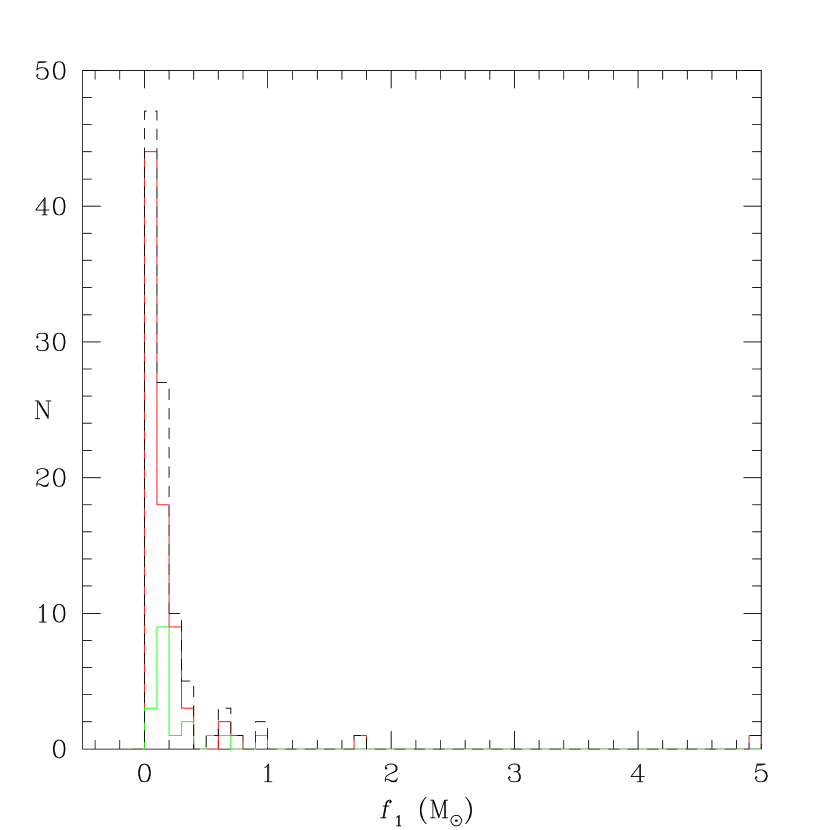
Figure 4.— Binary mass function distribution for red giant ellipsoidal variables in the LMC. The red line denotes our observation, the green line denotes the combined observations of Nicholls et al. (2010) and Nicholls & Wood (2012), and the black dashed line is the sum of the two distributions.

3.5. The PL Diagram

The variations of light amplitude, velocity amplitude and mass function across the PL diagram are shown in Figure 5. In the top panel, we can see that the higher-amplitude ellipsoidal variables tend to lie on the higher luminosity, shorter period side of sequence E. This is just as demonstrated by Soszyński et al. (2004) and is presumably because as the red giant in a binary system (with a given orbital period) evolves to higher luminosity, it will expand to a greater filling fraction of its Roche lobe and hence be more distorted and have a large light variation amplitude.

The middle panel of Figure 5 shows a tendency for higher- velocity amplitudes to be associated with shorter-period orbits, as might be expected. Of course, low-velocity amplitudes can be seen for shorter- period orbits if the orbital plane is oriented close to the plane of the sky: there are a few objects that seem to fall in this category.

The mass function also shows some correlation with position in the PL diagram (bottom panel of Figure 5). The most massive objects, with $f_{1}>0.8$ $\rm M_{\odot}$, lie on the upper part of sequence E in agreement with the results shown in Figure 1.

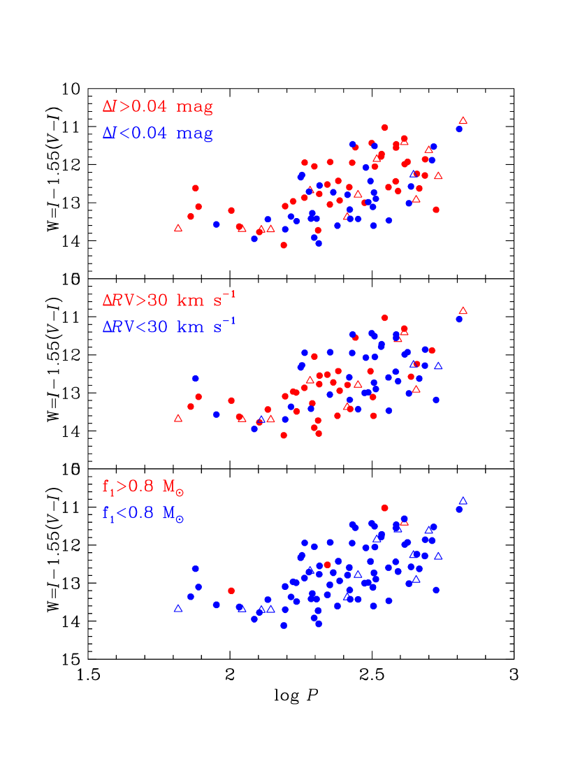
Figure 5.— PL diagram for the our 80 ellipsoidal variables. The top panel shows the position on the PL diagram of objects with different full-amplitude $\Delta I$, the middle panel shows the position of objects with different full-amplitude $\Delta\rm RV$ and the bottom panel shows the position of objects with different mass function $f_{1}$. In all panels, filled circles denote observations from this work and open triangles denote observations from Nicholls et al. (2010) and Nicholls & Wood (2012).

3.6. Velocity Amplitude versus Light Amplitude

In Figure 6, we present the light amplitude as a function of the velocity amplitude. Red symbols are our observation, and green symbols are observations from Nicholls et al. (2010) and Nicholls & Wood (2012). The 20 eccentric ellipsoidal variables from our observations and the 7 highly eccentric ellipsoidal variables studied by Nicholls & Wood (2012) are marked as open triangles. As expected, there is generally no correlation of the light and velocity amplitudes. The former depends on the Roche lobe filling factor (and inclination), while the latter depends on the stellar masses and the orbital separation. In principal, the orbital separation could influence the Roche lobe filling factor, but in practice the orbital separation effectively determines the luminosity on the giant branch where the Roche lobe nearly fills and ellipsoidal variability becomes detectable. This suggests that the orbital separation (velocity amplitude) should depend on luminosity for red giant ellipsoidal variables, but the light amplitude should not depend on orbital separation (velocity amplitude).

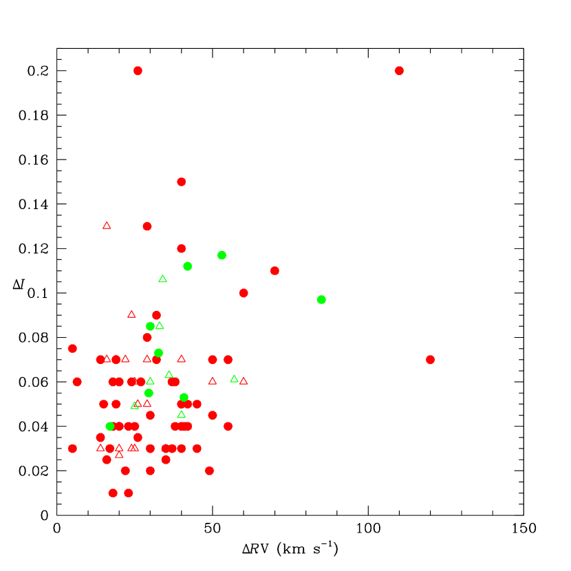
Figure 6.— Relation between the velocity amplitude and light amplitude. Red: observations from this work; circles are for circular binaries and triangles are for eccentric binaries. Green: observations from Nicholls et al. (2010) and Nicholls & Wood (2012); circles are for circular binaries and triangles are for eccentric binaries. Note that some objects are overwritten because they have the same velocity and light curve amplitude.

3.7. Velocity Amplitude versus Luminosity

As suggested in the last section, the velocity amplitude should show some correlation with luminosity. In Figure 7, we show the dependence of luminosity on velocity amplitude. The binaries with larger velocity amplitudes do tend to have lower luminosities although the effect is not prominent. This is as expected, since higher-velocity amplitude generally means a smaller separation and thus Roche lobe filling should occur at a lower luminosity.

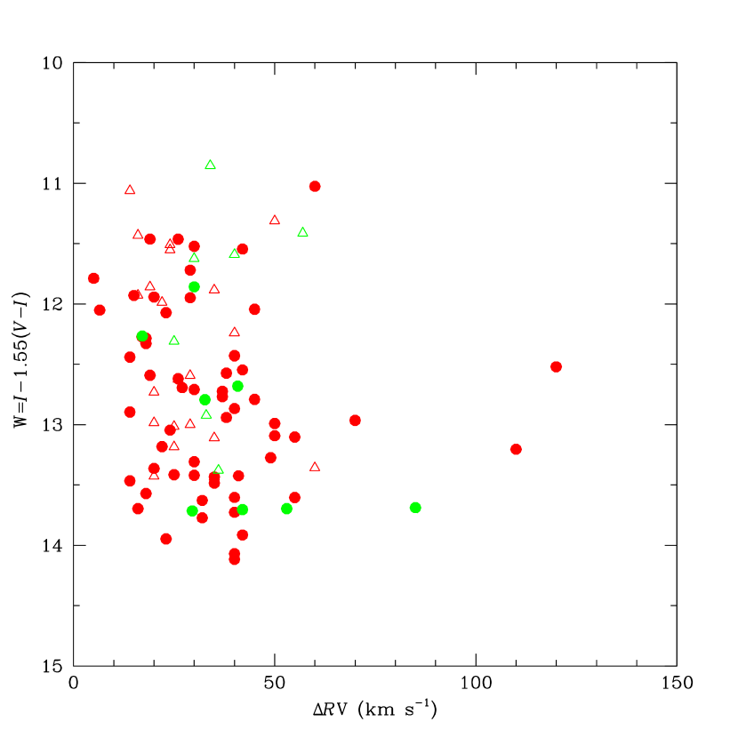
Figure 7.— Relation between velocity amplitude and luminosity. Symbols are as in Figure 6.

4. Summary and Conclusions

We have presented radial velocity observations obtained for 80 ellipsoidal red giant binaries in the LMC. This sample is much larger than the previous samples of Nicholls et al. (2010) and Nicholls & Wood (2012). The mass function of the sample suggests that the typical mass of the red giants in the ellipsoidal binaries is $\sim$1.35 M_⊙, in agreement with estimates derived from the star formation history of the LMC.

The main purpose of this paper was to present radial velocity data and basic observational properties of 80 ellipsoidal variables in the LMC. In future work, the radial velocity data will be combined with MACHO and OGLE photometric light curve data to give complete orbital solutions for these binary systems. This is possible because the distance, and hence the luminosity, of these LMC objects is well known (e.g. Nicholls & Wood, 2012). The results of the complete solutions will yield statistical distributions of masses, mass ratios, separations, and eccentricities in the period range observed. These distributions of orbital elements for binaries in the LMC can be compared with the solar vicinity statistical data given in the classic paper of Duquennoy & Mayor (1991) and the recent paper by Raghavan et al. (2010). It will be interesting to see if the same distributions exists in samples of binaries with different metallicity distributions and different star formation histories.

Appendix A List of objects rejected

Here we present data for the 6 objects that we removed from the 86 ellipsoidal candidates due to their poor velocity data relative to the noise. Properties of these 6 stars are given in Table 3, and their light and velocity curves are presented in Figure 8. Their velocity data is given in Table 1.

Table 3Properties of Objects Rejected

No	Object	$P$	$I$	$V$	$M_{B}$	$M_{R}$	$K$	$\Delta{I}$	$\Delta{\rm RV}$	$L$	$T_{\rm eff}$	$R$	Remark
	(OGLE II Name)	(day)	(mag)	(mag)	(mag)	(mag)	(mag)	(mag)	(km s-1)	($\rm L_{\odot}$)	(K)	($\rm R_{\odot}$)
1	050716.07-693259.7	563.3	14.81	16.18	-	-	13.09	0.025	-	1571	4368	70	1
2	051111.34-693714.9	147.7	15.69	17.41	-	-	13.59	0.060	-	772	3984	59	1
3	051150.57-685627.0	119.3	15.55	16.91	16.73	15.77	13.80	0.025	-	804	4344	51	1
4	052346.66-695140.6	259.0	15.34	16.77	-	-	13.54	0.050	-	983	4290	57	1,+sr,ogle3
5	053500.22-702643.4	286.5	15.19	16.71	16.60	15.52	13.34	0.060	-	1141	4225	64	1,ogle3
6	054109.54-704610.5	378.8	14.81	17.17	17.30	15.55	12.05	0.200	-	2298	3517	130	1,ogle3

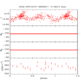
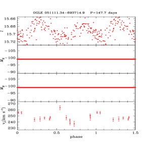
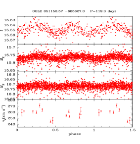
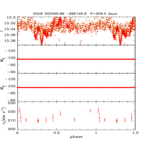
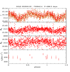
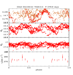
Figure 8.— Light and radial velocity curves of the 6 objects in the Appendix.

References

- Allen (1984) Allen, D. A. 1984, Proceedings of the Astronomical Society of Australia, 5, 369
- Adams, Wood, & Cioni (2006) Adams E., Wood P. R., Cioni M.-R., 2006, MmSAI, 77, 537
- Belczyński et al. (2000) Belczyński, K., Mikołajewska, J., Munari, U., Ivison, R. J., & Friedjung, M. 2000, A&AS, 146, 407
- Cutri et al. (2003) Cutri R. M., et al., 2003, yCat, 2246, 0
- Dopita et al. (2007) Dopita M., Hart J., McGregor P., Oates P., Bloxham G., Jones D., 2007, Ap&SS, 310, 255
- Dopita et al. (2010) Dopita M., et al., 2010, Ap&SS, 327, 245
- Duquennoy & Mayor (1991) Duquennoy A., Mayor M., 1991, A&A, 248, 485
- Fraser, Hawley, & Cook (2008) Fraser O. J., Hawley S. L., Cook K. H., 2008, AJ, 136, 1242
- Houdashelt et al. (2000a) Houdashelt M. L., Bell R. A., Sweigart A. V., Wing R. F., 2000a, AJ, 119, 1424
- Houdashelt et al. (2000b) Houdashelt M. L., Bell R. A., Sweigart A. V., 2000b, AJ, 119, 1448
- Ita et al. (2004) Ita Y., et al., 2004, MNRAS, 353, 705
- Kenyon (1986) Kenyon, S. J. 1986, Cambridge and New York, Cambridge University Press, 1986, 295 p.
- Keller & Wood (2006) Keller S. C., Wood P. R., 2006, ApJ, 642, 834
- Nicholls et al. (2009) Nicholls C. P., Wood P. R., Cioni M.-R. L., Soszyński I., 2009, MNRAS, 399, 2063
- Nicholls et al. (2010) Nicholls C. P., Wood P. R., Cioni M.-R. L., 2010, MNRAS, 405, 1770
- Nicholls & Wood (2012) Nicholls C. P., Wood P. R., 2012, MNRAS, 421, 2616
- Nie, Wood, & Nicholls (2012) Nie J. D., Wood P. R., Nicholls C. P., 2012, MNRAS, 423, 2764
- Mikolajewska et al. (1997) Mikolajewska, J., Acker, A., & Stenholm, B. 1997, A&A, 327, 191
- Madore (1982) Madore B. F., 1982, ApJ, 253, 575
- Raghavan et al. (2010) Raghavan D., et al., 2010, ApJS, 190, 1
- Rieke & Lebofsky (1985) Rieke G. H., Lebofsky M. J., 1985, ApJ, 288, 618
- Schlegel, Finkbeiner, & Davis (1998) Schlegel D. J., Finkbeiner D. P., Davis M., 1998, ApJ, 500, 525
- Stellingwerf (1978) Stellingwerf R. F., 1978, ApJ, 224, 953
- Soszyński et al. (2004) Soszyński I., et al., 2004, AcA, 54, 347
- Soszynski et al. (2007) Soszynski I., et al., 2007, AcA, 57, 201
- Wood et al. (1999) Wood P. R., et al., 1999, IAUS, 191, 151
- Wilson & Devinney (1971) Wilson R. E., Devinney E. J., 1971, ApJ, 166, 605
- Wilson et al. (2009) Wilson R. E., Chochol D., Komžík R., Van Hamme W., Pribulla T., Volkov I., 2009, ApJ, 702, 403
- Wilson (1979) Wilson R. E., 1979, ApJ, 234, 1054
- Wilson (1990) Wilson R. E., 1990, ApJ, 356, 613