Stability of equilibria of randomly perturbed maps
Abstract
We derive a sufficient condition for stability in probability of an equilibrium of a randomly perturbed map in . This condition can be used to stabilize weakly unstable equilibria by random forcing. Analytical results on stabilization are illustrated with numerical examples of randomly perturbed linear and nonlinear maps in one- and two-dimensional spaces.
1 Introduction
The idea of stabilizing unstable equilibria of dynamical systems by noise originates from the pioneering work of Khasminskii on stochastic stability in the nineteen-sixties [23]. Stochastic stabilization has important implications for control theory [7, 27, 5, 6] and for numerical methods for stochastic differential equations [29, 30, 18, 19, 12]. Furthermore, the interplay of stability and noise is important for understanding many dynamical phenomena in applied science including stochastic synchronization [1, 14, 28, 17], stochastic resonance [26, 25, 15], and noise-induced dynamics [8, 13, 20].
To illustrate the mechanism of stabilization in discrete setting, we consider a scalar difference equation
| (1.1) |
where and are independent copies of the random variable (RV) with zero mean and . Further, assume for some . The last condition is used to simplify the analysis. It can be replaced by a much weaker condition. For instance, it suffices to have .
For a given , we have
Let . Then with probability
and we have
holding almost surely. By the Strong Law of Large Numbers,
almost surely. Thus, the asymptotic stability of the origin (in the almost sure sense) will follow if
| (1.2) |
Using the Taylor expansion of and , we have
Thus, the stabilization of the weakly unstable equilibrium of (1.1) is achieved if
| (1.3) |
for . A similar stabilization condition is known for ordinary differential equations [23].
The stability analysis for (1.1) can be extended to linear maps in using the Furstenberg-Kesten theory [16]. For scalar nonlinear difference equations, stabilization was studied by Appleby, Mao, and Rodkina [6] and by Appleby, Berkolaiko, and Rodkina [4] (see also [2, 11, 3, 9]). Certain higher-dimensional models were analyzed in the context of stability of finite-difference schemes (see [12] and references therein). In this paper, we show that one can achieve stabilization with high probability for a general -dimensional nonlinear map under fairly general assumptions on the stabilizing perturbation. Specifically, we study the following difference equation in
| (1.4) |
where is a smooth function, and are deterministic and stochastic matrices respectively. We assume that the spectral radius of is slightly greater than , and ask how to choose mean-zero matrix to stabilize the equilibrium at the origin. Our motivation for considering (1.4) is two-fold. On one hand, we want to understand how to tame weak instability in general -dimensional maps by noise. Eventually, we want to apply these results to stabilize periodic orbits of randomly perturbed stochastic ordinary differential equations in . In this case, (1.4) represents a Poincare map [21]. Stochastic stabilization of period orbits remains largely unexplored area of research with many promising applications.
The organization of this paper is as follows. In the next section, we prove a sufficient condition for stability (in probability) of an equilibrium in a -dimensional map (cf. Theorem 2.2). To prove this theorem, we use the Strong Law of Large Numbers to show that the Lyapunov exponent of a typical trajectory is negative. The rest of the proof follows an argument developed for deterministic dynamical systems [24]. In §3 we apply Theorem 2.2 to the problem of stabilization. In §4, we illustrate our results with several numerical examples using one- and two-dimensional systems.
2 Stochastic stability
Consider an initial value problem for the following difference equation
| (2.5) |
where are independent copies of a random matrix ; is a continuous function such that
| (2.6) |
for some . Here and below, we will use to denote the Euclidean norm of a vector. The initial condition is assumed to be deterministic.
Definition 2.1.
Theorem 2.2.
Remark 2.3.
In (2.7), is an arbitrary matrix norm. The same matrix norm is used throughout this section.
Condition (2.7) guarantees that the largest Lyapunov exponent of a generic trajectory is negative. This implies stability of with high probability. Theorem 2.2 is a stochastic counterpart of the result of Koçak and Palmer for deterministic maps [24, Theorem 4]. It follows immediately from the proof of the following lemma, which also yields the rate of convergence of to the origin.
Lemma 2.4.
Proof: Suppose is arbitrary but fixed. Let and note that
by the Strong Law of Large Numbers [10, Theorem 22.1]. Thus, there exists such that
i.e., for
| (2.9) |
holds on the set of probability at least . In the remainder of the proof, we restrict to the realizations for which (2.9) holds.
Since is an integrable random variable, by Markov inequality, we have
Choosing sufficiently large, we have
| (2.12) |
The combination of (2.10), (2.11), and (2.12) yields
| (2.13) |
holding with probability at least , where depends on but not on or .
We are now in a position to prove (2.8). To this end, fix and choose such that
| (2.14) |
where . With these constants and , we will show (2.8) by induction.
The claim in (2.8) obviously holds for Let and suppose that
| (2.15) |
holds for We want to show that this entails
Iterating (2.5), we have
| (2.16) |
Using the triangle inequality, submultiplicativity of the matrix norm, and (2.6), from (2.16) we obtain
Here, we also used the induction hypothesis (2.15), which implies that so that (2.6) is applicable. Using (2.13), we further derive
Using the induction hypothesis (2.15), we continue
| (2.17) |
Next, we rewrite (2.17) in terms of
| (2.18) |
to obtain
By the discrete Gronwall’s inequality (see Lemma 2.5 below), we have
where we used (2.14) in the last inequality.
Recalling the definition of (2.18), we conclude that
Lemma 2.5.
3 Stabilization
Consider the following difference equation in :
| (3.1) |
where and is a matrix with the spectral radius
| (3.2) |
are independent copies of a random matrix . We want to identify the conditions on , which guarantee stabilization of the unstable equilibrium at the origin. To keep the notation simple, we will freely suppress the dependence of and on , whenever it is not essential.
Suppose the Jordan normal form of is
| (3.3) |
where is the block-diagonal matrix
| (3.4) |
for some . Block is if the corresponding eigenvalue of is real, or
otherwise. Therefore,
| (3.5) |
Here and below, stands for the operator norm of a matrix.
The upper-triangular matrix is nonzero only if has multiple eigenvalues. In this case, it has the following form
where is a zero block whose dimension coincides with that of for each . By changing coordinates, one can achieve
| (3.6) |
for any given in advance.111Indeed, let where is a identity matrix. Then all entries above the main diagonal of can be made arbitrarily small provided is large enough.
Thus, without loss of generality, we assume that matrix in (3.1) has the following form
| (3.7) |
where the block-diagonal matrix and the upper diagonal matrix are subject to (3.4), (3.5), and (3.6), respectively.
Next, we formulate our assumptions on the random matrix . First, we describe a general class of stabilizing random matrices. Later, we will see that in practice stabilization can be achieved with a very simple random matrix .
Let
| (3.8) |
where is a symmetric matrix, whose entries are mean zero non–degenerate RVs with finite third moments subject to the following conditions.
Denote
We assume
| (3.9) | |||
| (3.10) | |||
| (3.11) |
for some independent of .
Remark 3.1.
Condition (3.11) is easy to fulfill. For example, we may take , where is a mean–zero random variable with the finite third moment, . Then, for each such and , for some constant and (3.11) holds with for all . In particular, if are (arbitrarily dependent) standard normal random variables then (3.11) holds with .
By Theorem 2.2, for stabilization in (3.1) it is sufficient to show that the condition
| (3.12) |
holds for some small . The following lemma provides a sufficient condition for (3.12).
Lemma 3.2.
Remark 3.3.
The parametric dependence in (3.1) is used for convenience of presentation only. By interpreting as a function of , we are dealing with a single small parameter , instead of having to work with both and . The parametric dependence in (3.13) is not essential. What this condition means is that should be large enough compared to , while both and must be small.
Proof: By the submultiplicativity of the matrix norm and (3.8), we have
| (3.14) |
Let and whose values will be specified later be chosen. Using (3.7) and (3.5), from (3.14) we further obtain
| (3.15) |
By Gershgorin Theorem (cf. [22]),
By the monotonicity of logarithm,
Taking expectations on both sides, we get
For each
| (3.16) | |||||
By expanding the logarithm in the first term and using the fact that we get
| (3.17) |
Note that since for , the bound on the last term on the right–hand side of (3.17) gives the bound for the second term on the right–hand side in (3.16).
We estimate the terms above as follows
For and , as verified above. Further, for
Hence, by (3.9), (3.10), and (3.11) for all ,
Plugging all of this into (3.15) and using we obtain that
| (3.18) |
Let be any number strictly larger than . By (3.13) there exists an such that for all
Decreasing if necessary we may assume that the error term satisfies
Finally, for the chosen we choose a satisfying . With these choices the right–hand side of (3.18) is at most
This proves that the left–hand side of (3.18) is negative and completes the proof.
Remark 3.4.
As can be easily seen from the proof, for stabilization of the unstable equilibrium in (3.1) it is sufficient to take a diagonal matrix where mean zero RV meets the conditions on the three first moments (3.9) and (3.11) as well as (3.13). In particular, one can take , where is a standard normal RV and , but . Thus, in practice, it suffices to use a single RV to stabilize a weakly unstable equilibrium in .
a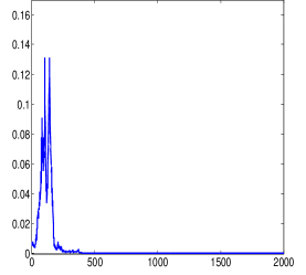 b
b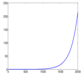
4 Examples
In this section, we illustrate our analysis of stabilization with several numerical examples.
4.1 One-dimensional maps
We consider first a scalar difference equation
| (4.1) |
where is a smooth function, , and are independent copies of a RV with .
Example 4.1.
Let and . The results of numerical simulations of (4.1) with the linear map above with small positive initial condition are shown in Figure 1. Plot a shows that the trajectory of the random system with noise intensity subject to (4.2) after a brief explosion converges to the origin. The deterministic trajectory in b grows exponentially.
Example 4.2.
Next, we consider a nonlinear map . For , the logistic map has two fixed points: and . For , the former is unstable, while the latter is stable. All trajectories of the deterministic map starting from converge to (see Fig. 2b). In the presence of noise, however, the iterations of (4.1) with high probability converge to provided (4.2) holds and is small enough (see Fig. 2a).
a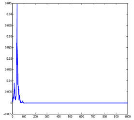 b
b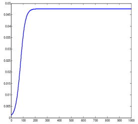
4.2 Two-dimensional maps
We next turn to the D case. To this effect, we consider
| (4.3) |
where is a deterministic matrix and
| (4.4) |
a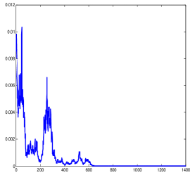 b
b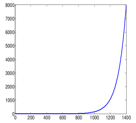
Example 4.3.
Example 4.4.
In this example, we consider a nonnormal matrix with multiple eigenvalues
Figure 4 shows the results of the stabilization by noise for this case. The experiments with the noise intensity in plots a and b show that stronger (albeit small) noise results in a more robust stabilization.
Acknowledgements. This work was supported in part by a grant from Simons Foundation (grant #208766 to PH) and by the NSF (grant DMS 1412066 to GM). GM has also benefitted from participating in a SQuaRe group ‘Stochastic stabilisation of limit-cycle dynamics in ecology and neuroscience’ sponsored by the American Institute of Mathematics.
a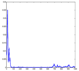 a
a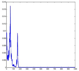 b
b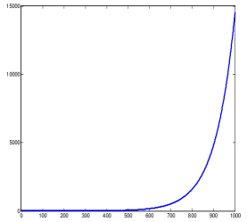
References
- [1] V.M. Afraĭmovich, N.N. Verichev, and M. I. Rabinovich, Stochastic synchronization of oscillations in dissipative systems, Izv. Vyssh. Uchebn. Zaved. Radiofiz. 29 (1986), no. 9, 1050–1060. MR 877439 (88g:58110)
- [2] J. Appleby, G. Berkolaiko, and A. Rodkina, On local stability for a nonlinear difference equation with a non-hyperbolic equilibrium and fading stochastic perturbations, J. Difference Equ. Appl. 14 (2008), no. 9, 923–951. MR 2439782 (2009g:39007)
- [3] J. Appleby, C. Kelly, X. Mao, and A. Rodkina, On the local dynamics of polynomial difference equations with fading stochastic perturbations, Dyn. Contin. Discrete Impuls. Syst. Ser. A Math. Anal. 17 (2010), no. 3, 401–430. MR 2656407 (2011d:39028)
- [4] J. Appleby, G. Berkolaiko, and A. Rodkina, Non-exponential stability and decay rates in nonlinear stochastic difference equations with unbounded noise, Stochastics 81 (2009), no. 2, 99–127. MR 2571683 (2010j:39028)
- [5] J. Appleby and X. Mao, Stochastic stabilisation of functional differential equations, Systems Control Lett. 54 (2005), no. 11, 1069–1081. MR 2170288 (2006d:34156)
- [6] J. Appleby, X. Mao, and A. Rodkina, On stochastic stabilization of difference equations, Discrete Contin. Dyn. Syst. 15 (2006), no. 3, 843–857. MR 2220752 (2007b:39031)
- [7] L. Arnold, Stabilization by noise revisited, Z. Angew. Math. Mech. 70 (1990), no. 7, 235–246. MR 1066866 (91j:93119)
- [8] N. Berglund and B. Gentz, Noise-induced phenomena in slow-fast dynamical systems, Probability and its Applications (New York), Springer-Verlag London, Ltd., London, 2006, A sample-paths approach. MR 2197663 (2007b:37115)
- [9] G. Berkolaiko and A. Rodkina, Almost sure convergence of solutions to nonhomogeneous stochastic difference equation, J. Difference Equ. Appl. 12 (2006), no. 6, 535–553. MR 2240374 (2007b:39002)
- [10] P. Billingsley, Probability and measure, 3rd ed., Wiley, 1995.
- [11] E. Braverman and A. Rodkina, On difference equations with asymptotically stable 2-cycles perturbed by a decaying noise, Comput. Math. Appl. 64 (2012), no. 7, 2224–2232. MR 2966858
- [12] E. Buckwar and C. Kelly, Towards a systematic linear stability analysis of numerical methods for systems of stochastic differential equations, SIAM J. Numer. Anal. 48 (2010), no. 1, 298–321. MR 2608371 (2011b:60271)
- [13] R.E.L. DeVille, E. Vanden-Eijnden, and C.B. Muratov, Two distinct mechanisms of coherence in randomly perturbed dynamical systems, Phys. Rev. E (3) 72 (2005), no. 3, 031105, 10. MR 2179903 (2006f:37074)
- [14] B. Doiron, J. Rinzel, and A. Reyes, Stochastic synchronization in finite size spiking networks, Phys. Rev. E (3) 74 (2006), no. 3, 030903, 4. MR 2282117 (2007k:92017)
- [15] M. Freidlin, On stochastic perturbations of dynamical systems with fast and slow components, Stoch. Dyn. 1 (2001), no. 2, 261–281. MR 1840196 (2003a:60032)
- [16] H. Furstenberg and H. Kesten, Products of random matrices, Ann. Math. Statist. 31 (1960), 457–469.
- [17] D.S. Goldobin and A. Pikovsky, Synchronization and desynchronization of self-sustained oscillators by common noise, Phys. Rev. E (3) 71 (2005), no. 4, 045201, 4. MR 2139983 (2005m:82085)
- [18] D.J. Higham, Mean-square and asymptotic stability of the stochastic theta method, SIAM J. Numer. Anal. 38 (2000), no. 3, 753–769 (electronic). MR 1781202
- [19] D.J. Higham, X. Mao, and C. Yuan, Almost sure and moment exponential stability in the numerical simulation of stochastic differential equations, SIAM J. Numer. Anal. 45 (2007), no. 2, 592–609 (electronic). MR 2300289 (2008c:60064)
- [20] P. Hitczenko and G.S. Medvedev, Bursting oscillations induced by small noise, SIAM J. Appl. Math. 69 (2009), no. 5, 1359–1392. MR 2487064 (2010f:60169)
- [21] , The Poincaré map of randomly perturbed periodic motion, J. Nonlinear Sci. 23 (2013), no. 5, 835–861. MR 3101836
- [22] R.A. Horn and C.R. Johnson, Matrix analysis, second ed., Cambridge University Press, Cambridge, 2013. MR 2978290
- [23] R. Khasminskii, Stochastic stability of differential equations, second ed., Stochastic Modelling and Applied Probability, vol. 66, Springer, Heidelberg, 2012, With contributions by G. N. Milstein and M. B. Nevelson. MR 2894052
- [24] H. Koçak and K.J. Palmer, Lyapunov exponents and sensitivity dependence, J. Dynam. Differential Equations 22 (2010), no. 3, 381–398. MR 2719912 (2012f:37075)
- [25] C. Laing and G.J. Lord (eds.), Stochastic methods in neuroscience, Oxford University Press, Oxford, 2010. MR 2640514 (2010m:60006)
- [26] A. Longtin, Neural coherence and stochastic resonance, Stochastic methods in neuroscience, Oxford Univ. Press, Oxford, 2010, pp. 94–123. MR 2642697
- [27] X. Mao, Stochastic stabilization and destabilization, Systems Control Lett. 23 (1994), no. 4, 279–290. MR 1298174 (95h:93089)
- [28] M. Porfiri and R. Pigliacampo, Master-slave global stochastic synchronization of chaotic oscillators, SIAM J. Appl. Dyn. Syst. 7 (2008), no. 3, 825–842. MR 2443024 (2009h:93117)
- [29] Y. Saito and T. Mitsui, Stability analysis of numerical schemes for stochastic differential equations, SIAM J. Numer. Anal. 33 (1996), no. 6, 2254–2267. MR 1427462 (98c:65138)
- [30] , Mean-square stability of numerical schemes for stochastic differential systems, Vietnam J. Math. 30 (2002), no. suppl., 551–560. MR 1964242 (2003m:65014)