Adiabatic hyperspherical analysis of realistic nuclear potentials

Abstract

Using the hyperspherical adiabatic method with the realistic nuclear potentials Argonne V14, Argonne V18, and Argonne V18 with the Urbana IX three-body potential, we calculate the adiabatic potentials and the triton bound state energies. We find that a discrete variable representation with the slow variable discretization method along the hyperradial degree of freedom results in energies consistent with the literature. However, using a Laguerre basis results in missing energy, even when extrapolated to an infinite number of basis functions and channels. We do not include the isospin $T=3/2$ contribution in our analysis.

1 Introduction

The hyperspherical adiabatic representation is well-established in atomic physics macek_properties_1968 ; lin_correlations_1974 . Few-nucleon problems have also taken advantage of this technique in solving simple model nuclear potentials garrido_integral_2012 . Though convergence with respect to the number of included channels is typically favorable in short-range low-energy atomic calculations wang_hyperspherical_2012 , we set out to check the convergence in the three-body nuclear problem. In particular, we test whether a typical orthogonal basis is flexible enough to handle the complicated nonadiabatic couplings.

The solution of the adiabatic Hamiltonian, eigenvalues (adiabatic potentials) and eigenvectors (channel functions) enters in the construction of a set of hyperradial equations that can be solved for bound or scattering states. This gives to the hyperspherical adiabatic representation a great flexibility. Most of the application of this technique has been done to determine bound state solutions, however in recent years several applications to determine scattering observables has been studied as well garrido_breakup_2014 .

In the present work, we use a hyperspherical harmonic basis to diagonalize the adiabatic Hamiltonian using the Argonne V14 (AV14) wiringa_nucleon-nucleon_1984 , Argonne V18 (AV18) wiringa_accurate_1995 , and AV18 with the Urbana IX (UIX) pieper_realistic_2001 three-body nuclear potentials. As a first step, to solve the adiabatic Hamiltonian we use a basis of symmetrized hyperspherical harmonics. In a second step, we solve the set of coupled hyperradial equations to determine the three-nucleon bound state using either a Laguerre polynomial basis or discrete variable representation (DVR). We compare the effectiveness of the two bases. This work can be seen as a first step in the application of the DVR technique, currently used in atomic physics, to the three-nucleon problem having in mind, as a final step, the treatment of the continuum spectrum.

Section 2 describes the hyperspherical coordinate description we use to solve the three-nucleon problem. Section 3 shows the solutions to the adiabatic Hamiltonian. Section 4 compares two methods in determining the three-body bound state and Sec. 5 concludes.

2 Theoretical background

We concern ourselves only with the relative Hamiltonian $H_{\rm rel}$. We recast $H_{\rm rel}$ in hyperspherical coordinates macek_properties_1968 ; lin_correlations_1974 in terms of five hyperangles denoted by $\vec{\Omega}$ and a single length, the hyperradius $R$. The relative Hamiltonian is then a sum of the hyperradial kinetic energy, the hyperangular kinetic energy, and the interaction potential,

$$H_{\rm rel}=-\frac{\hbar^{2}}{2m}\left(\frac{1}{R^{5}}\frac{\partial}{\partial R}R^{5}\frac{\partial}{\partial R}-\frac{\vec{\Lambda}^{2}}{R^{2}}\right)+V_{\rm int}(R,\vec{\Omega}).$$ (1)

Here, $m$ is the average nucleon mass and $\hbar$ is Planck’s constant. The exact form of the square of the grand angular momentum operator $\vec{\Lambda}^{2}$ depends on the choices of the Jacobi vectors and of the hyperangles and is not needed here.

The solution $\Psi_{E}(R,\vec{\Omega})$ to Eq. (1) is expanded in terms of the radial functions $R^{-5/2}F_{E\nu}(R)$ and the channel functions $\Phi_{\nu}(R;\vec{\Omega})$,

$$\Psi_{E}(R,\vec{\Omega})=R^{-5/2}\sum_{\nu}F_{E\nu}(R)\Phi_{\nu}(R;\vec{\Omega}).$$ (2)

The channel functions at a fixed hyperradius $R$ form a complete orthonormal set over the hyperangles,

$$\int\,d\vec{\Omega}\;\Phi^{*}_{\nu}(R;\vec{\Omega})\Phi_{\nu^{\prime}}(R;\vec{\Omega})=\delta_{\nu\nu^{\prime}},$$ (3)

and are the solutions to the adiabatic Hamiltonian $H_{\rm ad}(R,\vec{\Omega})$,

$$H_{\rm ad}(R,\vec{\Omega})\Phi_{\nu}(R;\vec{\Omega})=U_{\nu}(R)\Phi_{\nu}(R;\vec{\Omega}),$$ (4)

where

$$H_{\rm ad}= \frac{\hbar^{2}}{2m}\frac{\vec{\Lambda}^{2}+15/4}{R^{2}}+V_{\rm int}(R,\vec{\Omega}).$$ (5)

After applying Eq. (1) on the expansion Eq. (2) and projecting from the left onto the channel functions, the Schrödinger equation reads

$$\left(-\frac{\hbar^{2}}{2m}\frac{d^{2}}{dR^{2}}+U_{\nu}(R)-E\right)F_{E\nu}(R)$$ (6)

$$\qquad-\frac{\hbar^{2}}{2m}\sum_{\nu^{\prime}}\left(2P_{\nu\nu^{\prime}}(R)\frac{d}{dR}+Q_{\nu\nu^{\prime}}(R)\right)F_{E\nu^{\prime}}(R)=0.$$

The hyperspherical Schrödinger equation Eq. (6) is solved in a two step procedure. First, $H_{\rm ad}(R,\vec{\Omega})$ is solved parametrically in $R$ for the adiabatic potential curves $U_{\nu}(R)$. In a second step, the coupled set of one-dimensional equations in $R$ are solved. In Eq. (6), $P_{\nu\nu^{\prime}}$ and $Q_{\nu\nu^{\prime}}$ represent the coupling between channels, where

$$P_{\nu\nu^{\prime}}(R)=\bigg{\langle}\Phi_{\nu}\bigg{|}\frac{\partial\Phi_{\nu^{\prime}}}{\partial R}\bigg{\rangle}_{\vec{\Omega}}$$ (7)

and

$$Q_{\nu\nu^{\prime}}(R)=\bigg{\langle}\Phi_{\nu}\bigg{|}\frac{\partial^{2}\Phi_{\nu^{\prime}}}{\partial R^{2}}\bigg{\rangle}_{\vec{\Omega}}.$$ (8)

The brackets indicate that the integrals are taken only over the hyperangle $\vec{\Omega}$ with the hyperradius $R$ held fixed.

3 Adiabatic potential curves

We expand the channel functions, $\Phi_{\nu}(R;\vec{\Omega})$, using a basis of hyperspherical harmonics $\phi_{KM}(\vec{\Omega})$. Here, $K$ labels the grand angular momentum quantum number and $M$ labels the different degenerate states for a fixed $K$. The hyperspherical harmonics diagonalize the hyperangular kinetic energy operator, where $\vec{\Lambda}^{2}\phi_{KM}(\vec{\Omega})=K(K+4)\phi_{KM}(\vec{\Omega})$. The main challenge comes from calculating the potential matrix elements $\langle\phi_{KM}(\vec{\Omega})|V_{\rm int}|\phi_{KM}(\vec{\Omega})\rangle$ at a fixed hyperradius, which has been worked out by the second author using the technique of Ref. kievsky_high_1997 .

The hyperspherical harmonics are chosen to have certain symmetry properties. For example, subsets of basis functions are chosen to have orbital angular momenta $L_{12}$, $L_{12,3}$, and $L$. These correspond to the orbital angular momentum along the first Jacobi vector, the second Jacobi vector, and the total orbital angular momenta, respectively. Additionally, the spin $S_{12}$ and isospin $T_{12}$ along the first Jacobi vector, and the total spin $S$ and isospin $T$ are fixed. Other restrictions include that $L_{12}+S_{12}+T_{12}$ must be odd for antisymmetrization and $L$ and $S$ couple to $J=1/2$, the total angular momentum of the triton. In general, the sub-orbital angular momenta and spin are not good quantum numbers. Thus, the basis is not orthogonal and the adiabatic Hamiltonian, Eq. (5), is solved via a generalized eigenvalue problem at each hyperradius.

Table 1 shows an example of a set of basis functions.

Channel	$L_{12}$	$L_{12,3}$	$L$	$S_{12}$	$T_{12}$	$S$	$T$	$K_{min}$	$K_{\rm max}$
1	0	0	0	1	0	1/2	1/2	0	120
2	0	0	0	0	1	1/2	1/2	4	120
3	2	0	2	1	0	3/2	1/2	2	120
4	0	2	2	1	0	3/2	1/2	4	90
5	2	2	0	1	0	1/2	1/2	10	90
6	2	2	2	1	0	3/2	1/2	6	90
7	2	2	1	1	0	1/2	1/2	6	90
8	2	2	1	1	0	3/2	1/2	4	90
9	1	1	0	1	1	1/2	1/2	6	60
10	1	1	1	1	1	1/2	1/2	2	60
11	1	1	1	1	1	3/2	1/2	10	60
12	1	1	2	1	1	3/2	1/2	8	60
13	1	1	0	0	0	1/2	1/2	12	60
14	1	1	1	0	0	1/2	1/2	8	60
15	2	2	0	0	1	1/2	1/2	16	40
16	2	2	1	0	1	1/2	1/2	12	40
17	1	3	2	1	1	3/2	1/2	10	40
18	3	1	2	1	1	3/2	1/2	12	40

Table 1: Channel quantum numbers used in the hyperangular basis. $L_{12}$, $L_{12,3}$, and $L$, indicate the orbital angular momentum of the (12) pair, that of the third particle relative to the (12) pair, and the total. $S_{12}$ and $T_{12}$ indicate the spin and isospin of the (12) pair, while $S$ and $T$ are the total spin and isospin. $K_{min}$ ($K_{\rm max}$) is the minimum (maximum) grand hyperangular quantum number. The given values are used to generate data in Figs. 1(a), 2 and 3.

The different quantum numbers are listed in each column with a given set of channels labeled 1 through 18. The number of basis functions comes from the range of grand angular quantum numbers $K$ for each channel, where $K$ varies from $K_{min}$, to ensure linear independence, to $K_{\rm max}$ in steps of two to preserve parity. The total number of basis functions represented here is 617, where 227 have $L=0$, 185 have $L=1$, and 205 have $L=2$. This particular selection of channels and values of $K_{\rm max}$ describes the three-nucleon bound state with an accuracy of about $1$ keV kievsky_high_1997 .

The solid lines in Figure 1(a)

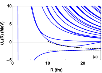
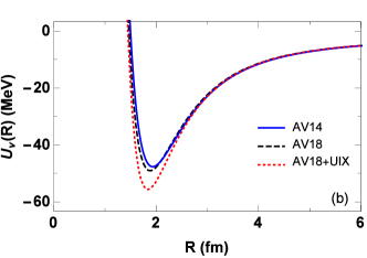
Figure 1: (Color online) Adiabatic potential curves. Panel (a) shows the adiabatic potential curves for the AV14 potential using the basis set in Table 1. The dashed lines show the known asymptotic limits for the two lowest potential curves, approaching the deuteron binding energy of -2.22MeV. Panel (b) shows the ground state adiabatic potential curves for three different nuclear potentials.

are the adiabatic potential curves generated from the basis in Table 1 for the AV14 nuclear potential. The full ground state potential curve can be seen in panel (b). There are a number of lines that asymptotically approach the zero energy threshold, indicating that these curves represent the fragmentation into three free particles. Two lines approach a negative energy threshold of -2.22MeV, such that these channels indicate the fragmentation into a deuteron and a free neutron. The two lowest potential curves are not converged, but the known asymptotic limits are indicated by dashed lines. In practice, the potentials are smoothly connected to their known asymptotic behavior. The lowest potential corresponds to an $s$-wave configuration between the deuteron and the neutron, where there is no angular momentum barrier. The second lowest potential corresponds to a $d$-wave configuration, where there is a significant angular momentum barrier.

It is known that the hyperspherical harmonic basis works well at small hyperradius, but requires a large number of basis functions to reach similar convergence at large hyperradius. We have seen that with the inclusion of more basis functions, e.g. going to 1052 basis functions with 362 at $L=0$, 335 at $L=1$, and 355 at $L=2$, that the lowest two potential curves in Fig. 1(a) are indistinguishable from their asymptotic behavior on the scale shown. Specifically, $K_{\rm max}$ is taken to be 150 for channels 1 to 6, 140 for channels 7 and 8, 110 for channels 9 to 14, and 90 for channels 15 to 18. Figure 1(b) uses this larger basis to show the lowest adiabatic potential curve for three different nuclear potentials. Solid, dashed, and dotted lines are for the AV14, AV18, and AV18 with UIX potentials, respectively. The difference between the different nuclear potentials is most clearly observed in the lowest adiabatic potential. The inclusion of the three-body potential, e.g., produces the lowest potential curve. On the scale shown in Fig. 1(a), there is no visible difference between the channels of the excited states. The next section describes the calculation of the bound state supported by the lowest adiabatic potentials.

4 Bound state energies

With the adiabatic potentials $U_{\nu}(R)$, we solve the hyperradial Schrödinger equation Eq. (6) to determine the bound state energy of the triton. As a first approach, we use a seven-point finite difference method to determine the $P$ and $Q$ matrix elements, together with a basis of Laguerre polynomials in the hyperradius $R$. There are two convergence criteria to consider. First, sufficiently many Laguerre polynomials must be used to describe the hyperradial wave functions. Second, sufficiently many channel functions must be included to reach convergence.

Figure 2(a)

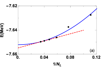
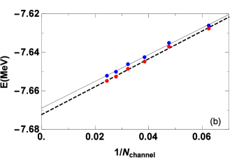
Figure 2: (Color online) Extrapolations used to estimate the triton energy for the AV14 potential using a Laguerre basis in the hyperradius. The upper panel shows the change in energy as a function of the number of Laguerre polynomials $N_{L}$ for 41 channel functions. The solid lines show strictly quadratic and linear fits to subsets of the data points. The lower panel shows the extrapolated values for different numbers of channel functions $N_{\rm channel}$. The upper and lower points (dashed and solid lines) correspond to the quadratic and linear fits, respectively. The lines show linear extrapolations to the infinite channel limit.

shows a convergence study for the AV14 potential as a function of the number of Laguerre basis functions $N_{L}$ with the lowest 41 channel functions included. The hyperangular basis used is that described in Table 1. The solid (dashed) line is a strictly quadratic (linear) fit to the data from $1/N_{L}=0.03$ to 0.12 (0.03 to 0.06). The two fits are used to estimate the energy assuming an infinite set of Laguerre basis functions. These extrapolations are calculated at different numbers of included channels $N_{\rm channel}$ and shown in Fig. 2(b). The upper (lower) points are from the quadratic (linear) extrapolations. Solid and dashed lines are linear fits to the data points of Fig. 2(b). Extrapolating to an infinite number of channels gives an estimate of $-7.671(2)$MeV for the triton binding energy.

This technique seems to miss about 10keV of binding energy when compared with other estimates perez_triton_2014 , or worse if estimating the energy by the last data point and not extrapolating to an infinite basis. We suggest that the error comes from the finite-difference method to calculate the $P$ and $Q$ matrix elements. The couplings show complicated behavior at small $R$ that may not be captured by this technique. We propose using a discrete variable representation light_generalized_1985 ; rescigno_numerical_2000 in $R$ together with the slow variable discretization method (SVD) tolstikhin_slow_1996 . Thus, the $P$ and $Q$ matrices are not needed since the hyperradial solution is solved in sectors that are exactly diagonalized. The only additional requirement is that the phase of each diagonalized sector must match between sector boundaries.

Figure 3

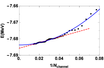
Figure 3: (Color online) Extrapolations used to estimate the triton energy for the AV14 potential using a DVR basis in the hyperradius with the SVD method. Solid and dashed lines show strictly quadratic and linear fits to the data points from $1/N_{\rm channel}$=[0,0.04].

shows the energy as a function of the number of included channels $N_{\rm channel}$. For this data, we use a total of 40 SVD sectors, with 20 ranging from $R=0.2$fm to 3fm and 20 ranging from $R=3$fm to 50fm. Each SVD sector consists of a DVR basis of five points. The hyperangular basis used is that described in Table 1. We find that the data changes in the fifth significant digit when we increase the number of DVR points to 10. Further, we find that the results are robust given changes in the number of sectors, so long as the potential minima is covered by enough points and the maximum range extends to the asymptotic limit at about 20fm. The solid (dashed) line of Fig. 3 is a strictly quadratic (linear) fit to the data including all points where $1/N_{\rm channel}<0.04$.

Compared to the Laguerre basis, we achieve a noticeably lower energy for the same number of included channels. Said differently, if we do not extrapolate to an infinite number of channels, the DVR energies would produce a better estimate than the Laguerre basis. The DVR basis is not a variational method, however, thus we include more channels in our DVR analysis (the left-most data point includes the 70 lowest channels). Regardless, the method shows a clear convergence and we estimate the triton binding energy to be $-7.685(1)$MeV.

The analysis is identical for the other nuclear potentials, with Fig. 3 being qualitatively similar for each. Using the larger hyperspherical basis described at the end of Sec. 3, we estimate the triton binding energy to be $-7.685(1)$MeV, $-7.619(2)$MeV, and $-8.475(2)$MeV for the AV14, AV18, and AV18 with UIX potentials, respectively. These results are in complete agreement with those given in the benchmark of Ref. nogga_three-nucleon_2003 showing the great flexibility of the SVD technique to treat the complexity of the adiabatic couplings.

5 Conclusion and Outlook

In this paper we calculated the adiabatic potentials curves for the three nucleon problem using realistic nuclear potentials in order to calculate the three-nucleon bound state. In calculating the triton binding energy, we find that the SVD method with a DVR basis gives results consistent with the literature nogga_three-nucleon_2003 , while using a naive finite-difference method leads to inconsistent results. This suggests that the channel couplings are handled well by the DVR basis.

Though the binding energy of three nucleons can be calculated by different techniques (see Ref. nogga_three-nucleon_2003 and references therein), this method may prove useful in calculating scattering data. As a preliminary study, we attempted to propagate the $R$ matrix in the SVD method, but the hyperspherical harmonic basis used does not produce convergence at large values of the hyperradius. This led to difficulties as we could not accurately connect the potentials and coupling matrix elements to their asymptotic behavior at large hyperradius in order to switch to a traditional $R$ matrix propagation method. To get around this limitation for scattering states below the three-nucleon breakup, we could use the method described in Ref. kievsky_theoretical_2012 , which only requires information from the bound state calculations in order to estimate the $S$ matrix elements. For determining the breakup amplitude a larger basis should be necessary in conjunction with the method described in Ref. garrido_breakup_2014 .

- (1) J. Macek, J. Phys. B: At. Mol. Opt. 1(5), 831 (1968).
- (2) C.D. Lin, Phys. Rev. A 10(6), 1986 (1974).
- (3) E. Garrido, C. Romero-Redondo, A. Kievsky, M. Viviani, Phys. Rev. A 86(5), 052709 (2012).
- (4) J. Wang, Hyperspherical approach to quantal three-body theory. Ph.D. thesis, University of Colorado, Boulder (2012)
- (5) E. Garrido, A. Kievsky, M. Viviani, Phys. Rev. C 90, 014607 (2014).
- (6) R.B. Wiringa, R.A. Smith, T.L. Ainsworth, Phys. Rev. C 29(4), 1207 (1984).
- (7) R.B. Wiringa, V.G.J. Stoks, R. Schiavilla, Phys. Rev. C 51(1), 38 (1995).
- (8) S. Pieper, Phys. Rev. C 64(1) (2001).
- (9) A. Kievsky, L.E. Marcucci, S. Rosati, M. Viviani, Few-Body Syst. 22(1), 1 (1997).
- (10) R.N. Pérez, E. Garrido, J.E. Amaro, E. Ruiz Arriola, Phys. Rev. C 90(4), 047001 (2014).
- (11) J.C. Light, I.P. Hamilton, J.V. Lill, J. Chem. Phys. 82(3), 1400 (1985).
- (12) T.N. Rescigno, C.W. McCurdy, Phys. Rev. A 62(3), 032706 (2000).
- (13) O.I. Tolstikhin, S. Watanabe, M. Matsuzawa, J. Phys. B: At., Mol. Opt. 29(11), L389 (1996).
- (14) A. Nogga, A. Kievsky, H. Kamada, W. Glöckle, L. Marcucci, S. Rosati, M. Viviani, Phys. Rev. C 67(3) (2003).
- (15) A. Kievsky, M. Viviani, L.E. Marcucci, Phys. Rev. C 85(1) (2012).