Curvatures and discrete Gauss-Codazzi equation in (2+1)-dimensional loop quantum gravity

Abstract

We derive the Gauss-Codazzi equation in the holonomy and plane-angle representations and we use the result to write a Gauss-Codazzi equation for a discrete (2+1)-dimensional manifold, triangulated by isosceles tetrahedra. This allows us to write operators acting on spin network states in (2+1)-dimensional loop quantum gravity, representing the 3-dimensional intrinsic, 2-dimensional intrinsic, and 2-dimensional extrinsic curvatures.

I Introduction

Three distinct notions of curvature are used in general relativity: the intrinsic curvature of the spacetime manifold, $M$, the intrinsic curvature of the spacial hypersurface $\Sigma$ embedded in $M$ which is utilised in the canonical framework, and the extrinsic curvature of $\Sigma$ key-1 . The three are related by the Gauss-Codazzi equation. On a discrete geometry, the definition of extrinsic curvature is not entirely clear key-2 . Even less so in loop quantum gravity (LQG), where the phase-space variables are derived from the first order formalism key-3 , which generically does not yield a direct interpretation as spacetime geometry. But a definition of these curvatures is important in LQG, because we expect a discrete (twisted) geometry to emerge from the theory in an appropriate semi-classical limit key-4 .

In $n$-dimensional discrete geometry, the manifold is formed by $n$-simplices key-2 ; key-5 . The intrinsics curvature sits on the $(n-2)$-simplices, called hinges, and can be defined by the angle of rotation: a vector parallel-transported around the hinge gets rotated by this angle. The rotation is in the hyperplane dual to the hinge.

In the canonical formulation of general relativity it is convenient to use the ADM formalism key-6 or a generalisation key-8 . The phase space variables are defined on an $n-1$ surface: the “initial time”, or, more generally, “boundary” surface $\Sigma$. At the core of the ADM formalism is the Gauss-Codazzi equation, relating the intrinsic curvature of the 4D spacetime with the intrinsic and extrinsic curvatures of $\Sigma$. In the context of a discrete geometry, $\Sigma$ is defined as an $(n-1)$-dimensional simplicial manifold formed by $(n-1)$-simplices. To develop a formalism analogous to the ADM one, we need an equation relating the intrinsic and extrinsic curvatures of $\Sigma$ and $M$, a ’discrete’ version of the Gauss-Codazzi equation.

In this paper, we explore a definition of extrinsic curvature for the discrete geometry which allows us to write an equation relating the extrinsic and intrinsics curvatures, which we refer as the Gauss-Codazzi equation for discrete geometry.

To get some insight into this problem, we first review the standard Gauss-Codazzi equation, both in second and first order formalism. In Section II we derive the holonomy (matrix) representation and plane-angle representation of the Gauss-Codazzi equation. We consider the discrete version of the Gauss-Codazzi equation in Section III, where we define all the curvatures. In Section IV, we move to the loop quantum gravity picture and study the operators corresponding to these curvatures into operators.

II Gauss-Codazzi equation

II.1 Standard Gauss-Codazzi equation

The Gauss-Codazzi equation relates the Riemann intrinsic curvatures of a manifold and its submanifold with the extrinsic curvature of the submanifold. We will briefly review the continuous (2+1)-dimensional Gauss-Codazzi equation in this section, but the formula will be valid in $(n+1)$-dimension.

II.1.1 Second order formulation

Consider a 3-dimensional manifold $M$ and a 2-dimensional surface $\Sigma$ embedded in $M$. In the second order formulation of general relativity key-7 , the Riemann intrinsic curvature of $M$ is a $\left(\begin{array}[]{c}1\\ 3\end{array}\right)$ tensor:

$$\,{}^{3}R=\,^{3}R_{\mu\nu\beta}^{\alpha}\partial_{\alpha}\wedge dx^{\beta}\otimes dx^{\mu}\wedge dx^{\nu},\qquad\alpha,\beta,\mu,\nu=0,1,2$$

which can be thought as a map that rotates a vector $v\in T_{p}M$ parallel-transported along an infinitesimal square loop defined by unit vectors $\left\{\partial_{\mu},\partial_{\nu}\right\}$. Next, we define the projection tensor as:

$$q_{\mu\nu}=g_{\mu\nu}-\left\langle n,n\right\rangle n_{\mu}n_{\nu},$$

with $n_{\mu}$ is the normal to hypersurface $\Sigma\subset M$. $\left\langle n,n\right\rangle=\pm 1$, depends on the signature of the metric. The projected Riemann curvature of $\,{}^{3}R$ on $\Sigma$ is defined as:

$$\left.\,{}^{3}R\right|_{\Sigma}=\,^{3}\widetilde{R}_{\mu\nu\beta}^{\alpha}\partial_{\alpha}\wedge dx^{\beta}\otimes dx^{\mu}\wedge dx^{\nu}=q_{\alpha^{\prime}}^{\alpha}q_{\mu}^{\mu^{\prime}}q_{\nu}^{\nu^{\prime}}q_{\beta}^{\beta^{\prime}}\,{}^{3}R_{\mu^{\prime}\nu^{\prime}\beta^{\prime}}^{\alpha^{\prime}}\partial_{\alpha}\wedge dx^{\beta}\otimes dx^{\mu}\wedge dx^{\nu}.$$

Taking the projected part $\left.\,{}^{3}R\right|_{\Sigma}$ from the full part $\,{}^{3}R$, we have relation as follow:

$$\,{}^{3}R=\left.\,{}^{3}R\right|_{\Sigma}+S,\qquad\left(\textrm{decomposition formula}\right),$$ (1)

$S$ is the ’residual’ part of $\,{}^{3}R.$ The projected part $\left.\,{}^{3}R\right|_{\Sigma}$ can be written as:

$$\left.\,{}^{3}R\right|_{\Sigma}=\,^{2}R+\left[K,K\right]\qquad\left(\textrm{Gauss equation}\right),$$ (2)

which can be written in terms of components:

$$\,{}^{3}\widetilde{R}_{\mu\nu\beta}^{\alpha}=\,^{2}R_{\mu\nu\beta}^{\alpha}+\left(K_{\mu}^{\alpha}K_{\beta\nu}-K_{\nu}^{\alpha}K_{\beta\mu}\right),\quad K_{\alpha\beta}=q_{\alpha}^{\mu}q_{\beta}^{\nu}\nabla_{\mu}n_{\nu}.$$ (3)

$\,{}^{2}R$ and $K$ are, respectively, the 2-dimensional Riemannian curvature and extrinsic curvature of hypersurface $\Sigma$. The residual part $S$ can be written as:

$$S_{\mu\nu\beta}^{\alpha}=n^{\alpha}\left(\,{}^{2}\nabla_{\nu}K_{\mu\beta}-\,^{2}\nabla_{\mu}K_{\nu\beta}\right)\qquad\left(\textrm{Codazzi equation}\right),$$

with $\,{}^{2}\nabla$ is the covariant derivative on the slice $\Sigma.$

Writing (1) and (2) together, we obtain:

$$\,{}^{3}R=\underset{\left.\,{}^{3}R\right|_{\Sigma}}{\underbrace{\,{}^{2}R+\left[K,K\right]}+S}.$$

II.1.2 First order formulation

The gravitational field is a gauge field and can be written in a form closer to Yang-Mills theory. This way of representing gravity is known as first order formulation of general relativity key-3 ; key-7 . Let manifold $M$ be a spacetime. Let $e$ be a local trivialization, a diffeomorphism map between the trivial vector bundle $M\times\mathbb{R}^{3}$ with the tangent bundle over $M$: $TM=\cup_{p}\left\{p\times T_{p}M\right\}$, and $A$ be the connection on $M\times\mathbb{R}^{3}$. The 3-dimensional intrinsic curvature of the connection is the curvature 2-form:

$$\,{}^{3}F=F_{\mu\nu J}^{I}\xi_{I}\wedge\xi^{J}\otimes dx^{\mu}\wedge dx^{\nu},\quad\mu,\nu,I,J=0,1,2.$$

which comes from the exterior covariant derivative of the connection:

$$F=d_{D}A.$$ (4)

$\left\{\partial_{\mu},dx^{\mu}\right\}$ and $\left\{\xi_{I},\xi^{I}\right\}$ are local coordinate basis on $M$ and $\mathbb{R}^{3},$ respectively. In terms of components:

$$F_{\mu\nu J}^{I}=\partial_{\mu}A_{\nu J}^{I}-\partial_{\nu}A_{\mu J}^{I}+A_{\mu K}^{I}A_{\nu J}^{K}-A_{\nu K}^{I}A_{\mu J.}^{K}$$ (5)

We use nice coordinates such that the time coordinate $\xi_{0}$ in fibre $\mathbb{R}^{3}$ is mapped by $e$ to the time coordinate $\partial_{0}$ in the basespace $M$, i.e., the map $e$ is fixed into:

$$e\left(\xi^{0}\right)=e^{0}=\delta_{\mu}^{0}dx^{\mu}=dx^{0}.$$

For the foliation, we use the time gauge, where the normal of the hypersurface $\Sigma$ is taken to be the time direction:

$$n=\partial_{0},\qquad e^{-1}\left(n\right)=\xi_{0}.$$

Then the $(2+1)$ split is simply carried by spliting the indices as $I=0,a,$ and $\mu=0,i,$ with $0$ as the temporal part:

$$\,{}^{3}F = \left(-F_{a0i0}+F_{00ia}+F_{ai00}-F_{0i0a}\right)\xi^{a}\wedge\xi^{0}\otimes dx^{i}\wedge dx^{0}+\left(F_{aij0}-F_{0ija}\right)\xi^{a}\wedge\xi^{0}\otimes dx^{i}\wedge dx^{j}+$$

$$+\left(F_{ai0b}-F_{a0ib}\right)\xi^{a}\wedge\xi^{b}\otimes dx^{i}\wedge dx^{0}+F_{aijb}\xi^{a}\wedge\xi^{b}\otimes dx^{i}\wedge dx^{j}$$

The projected part of the curvature 2-form on $\Sigma$ is:

$$\left.\,{}^{3}F\right|_{\Sigma}=F_{aijb}\xi^{a}\wedge\xi^{b}\otimes dx^{i}\wedge dx^{j},$$

and the residual part is:

$$S = \left(-F_{a0i0}+F_{00ia}+F_{ai00}-F_{0i0a}\right)\xi^{a}\wedge\xi^{0}\otimes dx^{i}\wedge dx^{0}+\left(F_{aij0}-F_{0ija}\right)\xi^{a}\wedge\xi^{0}\otimes dx^{i}\wedge dx^{j}$$

$$+\left(F_{ai0b}-F_{a0ib}\right)\xi^{a}\wedge\xi^{b}\otimes dx^{i}\wedge dx^{0}.$$

Therefore, the decomposition formula is clearly:

$$\,{}^{3}F=\left.\,{}^{3}F\right|_{\Sigma}+S.$$ (7)

Next, we take only the projected part:

$$\left.\,{}^{3}F\right|_{\Sigma}=F_{aijb}\xi^{a}\wedge\xi^{b}\otimes dx^{i}\wedge dx^{j},$$

which can be written in terms of components as follow:

$$F_{aijb}=\,^{2}F_{aijb}+A_{i0}^{a}A_{jb}^{0}-A_{j0}^{a}A_{ib}^{0}\qquad\textrm{(Gauss equation).}$$ (8)

The closed part of $\left.\,{}^{3}F\right|_{\Sigma}$ is clearly the 3D intrinsic curvature of connection in $\Sigma$ and the rest is the extrinsic curvature part:

$$\,{}^{2}F=\,^{2}F_{aijb}\xi^{a}\wedge\xi^{b}\otimes dx^{i}\wedge dx^{j}=\left(\partial_{i}A_{ajb}-\partial_{j}A_{aib}+A_{aic}A_{jb}^{c}-A_{ajc}A_{ib.}^{c}\right)\xi^{a}\wedge\xi^{b}\otimes dx^{i}\wedge dx^{j},$$

$$K=K_{i}^{a}\xi_{\alpha}\otimes dx^{i}=A_{i0}^{a}\xi_{\alpha}\wedge\xi^{0}\otimes dx^{i}.$$

The residual part $S,$ in this special coordinates and special gauge fixing satisfies:

$$F_{0ija}=\,^{2}D_{j}K_{ia}-\,^{2}D_{i}K_{ja}\qquad\textrm{(Codazzi equation),}$$

and the other temporal components are zero. It must be kept in mind that this is the Gauss-Codazzi equation for a special local coordinate and special choice of gauge fixing, for a general case, they are not this simple.

To conclude, we have the decomposition and Gauss-Codazzi equation for a fibre bundle of gravity:

$$\,{}^{3}F=\underset{\left.\,{}^{3}F\right|_{\Sigma}}{\underbrace{\,{}^{2}F+\left[\,{}^{2}K,\,^{2}K\right]}+S.}$$

II.2 Gauss-Codazzi equation in holonomy representation

II.2.1 Holonomy around a loop

In this section, we will write the Gauss-Codazzi equation in terms of holonomy. The holonomy is defined by the parallel transport of any section of a bundle, say, $s_{0}$, so that it satisfies the equation as follow:

$$D_{v}\left(s_{0}\right) =\partial s_{0}+A\left(s_{0}\right)= 0.$$ (9)

Solving (9) using recursive method key-3 ; key-7 ; key-8 , we obtain the solution:

$$s\left(t\right)=U\left(\gamma\left(t\right),D\right)s_{0},$$

$U\left(\gamma\left(t\right),D\right)$ is holonomy of connection $D$ along path $\gamma\left(t\right)$:

$$U\left(\gamma\left(t\right),D\right)=U_{\gamma}\equiv{P}\exp\int A,$$ (10)

with ${P}$ is the path-ordered operator (See key-3 ; key-8 for the details of the derivation).

Consider a square loop $\gamma$ embedded in $\Sigma$ which encloses a 2-dimensional area. The holonomy around the square loop can be written as a product of four holonomies, since holonomy is piecewise-linear:

$$U_{\gamma}=U_{\gamma_{4}}U_{\gamma_{3}}U_{\gamma_{2}}U_{\gamma_{1},}$$

Taylor expanding the holonomy in (10) up to the second order key-3 ; key-7 ; key-9 , we obtain:

$$U_{\gamma}=1+\frac{a^{\mu\nu}}{2}F_{\mu\nu}+\mathcal{O}^{4},$$

with $a^{\mu\nu}$ is an infinitesimal square area inside loop $\gamma.$ The formula:

$$\frac{a^{\mu\nu}}{2}F_{\mu\nu}=U_{\gamma}-1-\mathcal{O}^{4}$$ (11)

will be used to write the Gauss-Codazzi equation in terms of holonomies.

II.2.2 First order formulation in holonomy representation

Contracting (II.1.2) by an infinitesimal area $a^{\mu\nu}$, we obtain:

$$\frac{a^{\mu\nu}}{2}\,^{3}F_{I\mu\nu J} =\,^{3}U_{IJ}-\delta_{IJ}-\mathcal{O}^{4}= \frac{a^{i0}}{2}\left(-F_{a0i0}+F_{00ia}+F_{ai00}-F_{0i0a}\right)\xi^{a}\wedge\xi^{0}+\frac{a^{ij}}{2}\left(F_{aij0}-F_{0ija}\right)\xi^{a}\wedge\xi^{0}+$$

$$+\frac{a^{i0}}{2}\left(F_{ai0b}-F_{a0ib}\right)\xi^{a}\wedge\xi^{b}+\frac{a^{ij}}{2}F_{aijb}\xi^{a}\wedge\xi^{b},$$

where we have used the result in (11), relating the holonomy with the curvature of the connection. Taking the projected part (8) contracted with $a^{ij},$ and using the relation between holonomy with the curvature 2-form, we can write the projected part in terms of 2-dimensional holonomy and the contracted extrinsic curvature as follow:

$$\frac{a^{ij}}{2}F_{aijb} = \frac{a^{ij}}{2}\,^{2}F_{aijb}+\frac{a^{ij}}{2}\left(K_{ai}K_{jb}-K_{aj}K_{ib}\right)=\,^{2}U_{ab}-\delta_{ab}-\mathcal{O}^{4}+\frac{a^{ij}}{2}\left(K_{ai}K_{jb}-K_{aj}K_{ib}\right).$$

Finally, collecting all these result together, we obtain:

$$\underset{\left(\,{}^{3}U_{IJ}-\delta_{IJ}-\mathcal{O}^{4}\right)\xi^{I}\wedge\xi^{J}}{\underbrace{\frac{a^{\mu\nu}}{2}\,^{3}F_{I\mu\nu J}\xi^{I}\wedge\xi^{J}}} = \underset{\left(\,{}^{2}U_{ab}-\delta_{ab}-\mathcal{O}^{4}\right)\xi^{a}\wedge\xi^{b}}{\underbrace{\frac{a^{ij}}{2}\,^{2}F_{aijb}\xi^{a}\wedge\xi^{b}}}+\underset{\left[K,K\right]_{ab}\xi^{a}\wedge\xi^{b}}{\underbrace{\frac{a^{ij}}{2}\left(K_{ai}K_{jb}-K_{aj}K_{ib}\right)\xi^{a}\wedge\xi^{b}}}$$

$$\left.\begin{array}[]{c}+\frac{a^{i0}}{2}\left(\left(-F_{a0i0}+F_{00ia}+F_{ai00}-F_{0i0a}\right)\xi^{a}\wedge\xi^{0}+\left(F_{ai0b}-F_{a0ib}\right)\xi^{a}\wedge\xi^{b}\right)\\ +\frac{a^{ij}}{2}\left(F_{aij0}-F_{0ija}\right)\xi^{a}\wedge\xi^{0}\end{array}\right\}S,$$

or simply:

$$\,{}^{3}U=\,^{2}U+\underset{T}{\underbrace{\left[K,K\right]+S+\left(\,{}^{3}I-\,^{2}I\right)}},$$ (13)

where we have written the Gauss-Codazzi and the decomposition formula together, noting the residual terms as $S$. Remember that $U$ is the holonomy of the connection, which describes the curvature of the connection of fibre $F$, not the curvature of the basespace $M$.

II.2.3 Second order formulation in holonomy representation

In the same manner as above, for a tangent bundle $TM$, we obtain the relation

$$\underset{\left(\,{}^{3}H_{\alpha\beta}-\delta_{\alpha\beta}-\mathcal{O}^{4}\right)dx^{\alpha}\wedge dx^{\beta}}{\underbrace{\frac{a^{\mu\nu}}{2}\,^{3}R_{\alpha\mu\nu\beta}dx^{\alpha}\wedge dx^{\beta}}} = +\underset{\left(\,{}^{2}H_{kl}-\delta_{kl}-\mathcal{O}^{4}\right)dx^{k}\wedge dx^{l}}{\underbrace{\frac{a^{ij}}{2}\,^{2}R_{kijl}dx^{k}\wedge dx^{l}}}+\underset{\left[K,K\right]_{kl}dx^{k}\wedge dx^{l}}{\underbrace{\frac{a^{ij}}{2}\left(K_{ki}K_{jl}-K_{kj}K_{il}\right)dx^{k}\wedge dx^{l}}}$$

$$\left.\begin{array}[]{c}+\left(\frac{a^{i0}}{2}\left(-R_{j0i0}+R_{00ij}+R_{ji00}-R_{0i0j}\right)+\frac{a^{ij}}{2}\left(R_{jik0}-R_{0ikj}\right)\right)dx^{j}\wedge dx^{0}\\ +\frac{a^{i0}}{2}\left(R_{ji0k}-R_{j0ik}\right)dx^{j}\wedge dx^{k}\end{array}\right\}S,$$

or simply:

$$\,{}^{3}H=\,^{2}H+\underset{T}{\underbrace{\left[K,K\right]+S+\left(\,{}^{3}I-\,^{2}I\right)}},$$ (15)

with $H$ is the holonomy around any loop $\gamma$ embedded in $\Sigma\subseteq M$, coming from the Riemann tensor $R$.

II.3 Gauss-Codazzi equation in plane-angle representation

Rotations can be represented in two ways, using the holonomy (matrix) representation, or using the plane-angle representation. For a continuous theory, the holonomy representation provides a simpler way to do calculation concerning rotation. In a discrete theory, where we would like to get rid of coordinates, the plane-angle representation is a natural way to represent rotations and curvatures. The plane-angle representation is only a representation of the rotation group using its Lie algebra for the plane of rotation and one (real) parameter group times the norm of the algebra for the angle of rotation. There exist a bijective map sending the holonomy to the plane-angle representation, known as the exponential map key-10 .

In this section, we rewrite the Gauss-Codazzi equation using the plane-angle representation. We only do the calculation for the second order formalism, the first order formalism version can be obtained in a similar way. Firstly, let us define the variables; we have two equations: the decomposition formula and the Gauss-Codazzi equation written compactly in (15). Since we are working in (2+1)-dimension, it is natural to use matrix group $SO(3)$ to represents the 3-dimensional intrinsic curvature, and the subgroup $SO(2)$ to represents the 2-dimensional intrinsic curvature. But for simplicity of the calculation, we use the unitary group $SU(2)$ –the double cover of $SO(3)$– instead of $SO(3)$. Having information of $\,{}^{3}H\in SU(2)$ is equivalent with having information of the plane and angle of the 3-dimensional rotation, which are denoted, respectively, by $\left\{J\in\mathfrak{su(2)},\delta\theta\in\mathbb{R}\right\}$. The same way goes with $\,{}^{2}H\in SO(2)$, it contains same amount of information with the plane-angle of the 2-dimensional rotation $\left\{j\in\mathfrak{so(2)},\delta\phi\in\mathbb{R}\right\}$. Using the exponential map, we can write:

$${}^{2}H=\exp\left(j\delta\phi\right)=I_{2\times 2}\cos\delta\phi+j\sin\delta\phi,$$ (16)

with

$$j=\left[\begin{array}[]{cc}0&1\\ -1&0\end{array}\right],$$ (17)

is the generator of $SO(2).$ Doing the same way to the element of $SU(2)$, we obtain:

$${}^{3}H\sim\exp\left(J\delta\theta\right)=I_{2\times 2}\cos\frac{\delta\theta}{2}+J\sin\frac{\delta\theta}{2},$$ (18)

with $J\in\mathfrak{su(2)}$ is an element of the Lie algebra of SU(2), satisfying:

$$J=J^{a}\bar{\sigma}_{a},\quad J^{a}J_{a}=1.$$

$\bar{\sigma}_{a}$ are the basis of $\mathfrak{su(2),}$ namely, the generator of $SU(2)$:

$$\bar{\sigma}_{a}=i\sigma_{a},$$

satisfying the algebra structure relation as follow:

$$\left[\bar{\sigma}_{a},\bar{\sigma}_{b}\right]=-2\varepsilon_{ab}^{\>\,c}\bar{\sigma}_{c},$$ (19)

with $\sigma_{a}$ are the Pauli matrices:

$$\sigma_{x}=\left[\begin{array}[]{cc}0&1\\ 1&0\end{array}\right],\quad\sigma_{y}=\left[\begin{array}[]{cc}0&-i\\ i&0\end{array}\right],\quad\sigma_{z}=\left[\begin{array}[]{cc}1&0\\ 0&-1\end{array}\right]$$

The $\frac{1}{2}$ factor in (18) comes out from the normalization occuring when we write $SO(3)$ using $SU(2)$ representation, i.e., to reduce the factor 2 in relation (19)

Taking the trace of (15) gives the relation between 3-dimensional and 2-dimensional rotation angle:

$$\underset{2\cos\frac{\delta\theta}{2}}{\underbrace{\textrm{tr}\,^{3}H}}=\underset{2\cos\delta\phi}{\underbrace{\textrm{tr}\,^{2}H}}+\textrm{tr}T,$$ (20)

using the fact that the elements of the algebra are skew-symmetric. The other relation we need to have the full information contained by (15) is the planes of rotation. Since the embedded surface is 2-dimensional, the plane of rotation for $\delta\phi$ is trivial, which is (17). The plane of rotation $J$ for $\delta\theta$ can be obtained by solving complex $2\times 2$ matrix linear equation (18):

$$J=\frac{{}^{3}H-I_{2\times 2}\cos\frac{\delta\theta}{2}}{\sin\frac{\delta\theta}{2}}.$$ (21)

In conclusion, the contracted Gauss-Codazzi equation concerning the relation of curvatures of a manifold and its submanifold in (2+1) dimension can be written using holonomy representation (15) or using the plane-angle representation, i.e., the relation between rotation angles by (20) and the condition for the planes of rotation, by (17) and (21).

III Discrete (2+1) geometry

III.1 Geometrical setting

Using the Gauss-Codazzi equation in terms of holonomy and plane-angle representation obtained in the previous section, we can write the Gauss-Codazzi equation for discrete (2+1) geometry; this is the objective of this section. Let a portion of curved 3-dimensional manifold $M$ be discretized by flat tetrahedra, we call this discretized manifold $M_{\triangle}$. See FIG. 1.

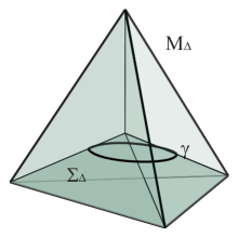
Figure 1: Suppose we have a 3-dimensional curved manifold $M_{\triangle}$ discretized by four tetrahedron in the figure above (in flat case it is known as 1-4 Pachner move). Then we take an embedded slice $\Sigma_{\triangle}$ as the surface of one tetrahedron (the dark blue surface discretized by three triangle). Embedded on $\Sigma_{\triangle},$ we take a loop $\gamma$ circling a point of a tetrahedron. Attached to $\gamma$, are the $SU(2)$ and $SO(2)$ holonomy, which are related to the 3D and 2D intrinsic curvature, respectively.

III.1.1 Angle relation

In this section we derive the Gauss-Codazzi equation purely from the angles between simplices, i.e, the relation between geometrical objects, without reference to coordinates (this is, indeed, the reason Tullio Regge developed his Regge calculus and discrete general relativity, in his famous paper titled ’General relativity without coordinates’ key-5 ). There are two kinds of relevant angles in a flat tetrahedron: the ’angle at a vertex’ between two segments of the tetrahedron meeting at a vertex, which we denote $\phi$; and the ’dihedral angle at a segment’, namely the angle between two triangles, which we denote $\theta$. These two types of angles are related by the ’angle formula of the tetrahedron’:

$$\cos\theta_{abac}=\frac{\cos\phi_{bc}-\cos\phi_{ab}\cos\phi_{ac}}{\sin\phi_{ab}\sin\phi_{ac}}.$$ (22)

See FIG. 2.

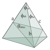
Figure 2: Given angles $\phi_{ab}$, $\phi_{bc}$, $\phi_{ca}$ at point $p$ of a tetrahedron, we could obtain the dihedral angle $\theta_{abac}$. In fact, $\theta_{abac}$ is only $\phi_{bc}$ projected on the plane normal to segment $a$.

III.1.2 Isosceles tetrahedron

For simplicity of the derivation in the next section, we consider isosceles tetrahedron. An isosceles tetrahedron is build by three isosceles triangles and one equilateral triangle. In this case, all angles around one point $p$ of the tetrahedron are equal, say $\phi_{i}=\phi$, and the dihedral angle relation (22) becomes:

$$\cos\theta = \frac{\cos\phi}{\left(1+\cos\phi\right)}.$$

This implies that the dihedral angles between two isosceles triangles are equal as well, say $\theta_{i}=\theta$. Another geometrical property of a tetrahedron which is useful for the derivation in this section is the volume. The volume of unit isosceles parallelepiped is:

$$\textrm{vol}=\left(\vec{n}_{1}\times\vec{n}_{2}\right)\cdot\vec{n}_{3}=\frac{1}{3}\left(1-\cos\phi\right)\sqrt{1+2\cos\phi}=\frac{1}{3}\left(\sin^{2}\frac{\phi}{2}\right)\sqrt{4\cos^{2}\frac{\phi}{2}-1}.$$ (23)

III.2 Curvatures in discrete geometry

In $n$-dimensional discrete geometry, the notion of curvature is represented using the plane-angle representation. The intrinsic curvature is represented by the angle of rotation, which in this case is called as deficit angle, and this deficit angle is located on the hinge, the $(n-2)$ form duals to the plane of rotation. The geometrical interpretation of deficit angle is illustrated by the FIG. 3.

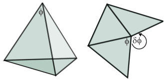
Figure 3: Suppose $\Sigma_{\Delta}$ is a 2D surface discretized by three triangles. Point $p$ is the hinge where the deficit angle $\delta\phi$ is located. $\delta\phi$ is the 2D intrinsic curvature of $\Sigma_{\Delta}$ at point $p$.

To obtain the 2-dimensional and 3-dimensional intrinsic curvatures in discrete geometry picture, firstly we need to define a discretized surface embedded in $M_{\Delta},$ say $\Sigma_{\Delta}.$ The simplest way is to take the surface of the tetrahedron as a slice (see FIG. 1). Having $\Sigma_{\Delta}$ embedded on $M_{\Delta}$, we consider a loop $\gamma$ on $\Sigma_{\Delta}.$ We consider the holonomy related to the 2D and 3D curvatures defined by this loop. The 3D curvature is defined by the 3D holonomy ${}^{3}H\in SO(3)\sim SU(2)$ around loop $\gamma$, which describes the intrinsic curvature of $M_{\Delta},$ while the 2D curvature is the 2D holonomy ${}^{2}H\in SO(2),$ describing the intrinsic curvature of slice $\Sigma_{\Delta}$, still along the same loop. Taking trace of the holonomies, we obtain the angles of rotation, i.e., the amount of a components of a vector parallel to the plane of rotation get rotated when parallel transported along loop $\gamma$. In discrete geometry, this rotation angle is the same as the deficit angle on the hinges.

III.2.1 2D intrinsic curvature $(SO(2))$

Using FIG. 4 as the simplest case, we take loop $\gamma$ circling point $p$ on the surface $\Sigma$, therefore the 2D curvature is the deficit angle on $p$:

$${}^{2}R=\delta\phi=2\pi-\sum_{i}\phi_{i},$$ (24)

or in terms of the cosine function:

$$\cos\delta\phi=\prod_{i=1}^{3}\cos\phi_{i}-\sum_{i=1,i\neq j,k,j<k}^{3}\cos\phi_{i}\sin\phi_{j}\sin\phi_{k}.$$ (25)

For the isosceles tetrahedron case, (24)-(25) become:

$${}^{2}R=\delta\phi=2\pi-3\phi,$$

$$\cos\delta\phi=\cos^{3}\phi-3\cos\phi\sin^{2}\phi=\cos\phi\left(4\cos^{2}\phi-3\right).$$

We could obtain the holonomy by the exponential map (16), using the $SO(2)$ algebra (17).

III.2.2 3D intrinsic curvature $(SU(2))$

We could write 3D curvature by the holonomy of SU(2) using (18), but the 3-dimensional holonomy along loop $\gamma$ circling point $p$ is a product of three holonomies on the three hinges, because the loop crosses three hinges. See FIG. 4.

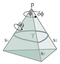
Figure 4: A portion of a discretized curved manifold $M_{\Delta}$ with an embedded discretized hypersurface $\Sigma_{\Delta}$. It is clear that the loop $\gamma$ circles point $p$, where the 2D deficit angle $\delta\phi$ is located. $\delta\phi$ represents 2D intrinsic curvature since it is located on a point. The loop also crosses 3 segments which are $s_{1}$, $s_{2}$, $s_{3}.$ Each segments contains its own 3D deficit angle $\delta\theta,$ which represent 3D intrinsic curvature since it is located on a line. Using the exponential map, we can obtain holonomies on each line corresponding to the deficit angles. From these holonomies, we can obtain the 3D total holonomy along loop $\gamma$, which is the product of holonomies on the 3 segments.

$${}^{3}H=\prod_{i=1}^{3}{}^{3}H_{i}$$ (26)

Using (18), we obtain:

$${}^{3}H = \prod_{i=1}^{3}\left(I\cos\frac{\delta\theta_{i}}{2}+J_{i}\sin\frac{\delta\theta_{i}}{2}\right)$$

$$= I\prod_{i=1}^{3}\cos\frac{\delta\theta_{i}}{2}+\sum_{i=1,i\neq j,k,j<k}^{3}J_{i}\sin\frac{\delta\theta_{i}}{2}\cos\frac{\delta\theta_{j}}{2}\cos\frac{\delta\theta_{k}}{2}+\sum_{i=1,i<j,i,j\neq k}^{3}J_{i}\sin\frac{\delta\theta_{i}}{2}J_{j}\sin\frac{\delta\theta_{j}}{2}\cos\frac{\delta\theta_{k}}{2}+\prod_{i=1}^{3}J_{i}\sin\frac{\delta\theta_{i}}{2},$$

where each hinge (segment) $i$ is dual to plane $J_{i}=\vec{J}_{i}\cdot\hat{\bar{\sigma}}$ and is attached by a deficit angle $\delta\theta_{i}$. Taking trace of the equation above gives:

$$\underset{2\cos\frac{\delta\Theta}{2}}{\underbrace{\textrm{tr}{}^{3}H}} =\underset{2}{\underbrace{\textrm{tr}I}}\prod_{i=1}^{3}\cos\frac{\delta\theta_{i}}{2}+\sum_{i=1,i\neq j,k,j<k}^{3}\underset{0}{\underbrace{\textrm{tr}J_{i}}}\sin\frac{\delta\theta_{i}}{2}\cos\frac{\delta\theta_{j}}{2}\cos\frac{\delta\theta_{k}}{2}+\sum_{i=1,i<j,i,j\neq k}^{3}\underset{-2\left(\vec{J}_{i}\cdot\vec{J}_{j}\right)}{\underbrace{\textrm{tr}\left(J_{i}J_{j}\right)}}\sin\frac{\delta\theta_{i}}{2}\sin\frac{\delta\theta_{j}}{2}\cos\frac{\delta\theta_{k}}{2}$$

$$+\underset{+2\left(\vec{J}_{1}\times\vec{J}_{2}\right)\cdot\vec{J}_{3}}{\underbrace{\textrm{tr}\left(\prod_{i=1}^{3}J_{i}\right)}}\prod_{i=1}^{3}\sin\frac{\delta\theta_{i}}{2},$$

or simply:

$$\cos\frac{\delta\Theta}{2}=\prod_{i=1}^{3}\cos\frac{\delta\theta_{i}}{2}-\sum_{i=1,i<j,i,j\neq k}^{3}\left(\vec{J}_{i}\cdot\vec{J}_{j}\right)\sin\frac{\delta\theta_{i}}{2}\sin\frac{\delta\theta_{j}}{2}\cos\frac{\delta\theta_{k}}{2}+\left(\vec{J}_{1}\times\vec{J}_{2}\right)\cdot\vec{J}_{3}\sin\frac{\delta\theta_{i}}{2},$$

But $\left(\vec{J}_{i}\cdot\vec{J}_{j}\right)=\cos\phi_{i}$, and $\left(\vec{J}_{1}\times\vec{J}_{2}\right)\cdot\vec{J}_{3}$ is just the volume of the parallelepiped defined by $\left\{\vec{J}_{1},\vec{J}_{2},\vec{J}_{3}\right\}$. (Remember that $\vec{J}=\star J$, or 1-form $\vec{J}$ is the Hodge dual of the 2-form $J$ in 3-dimensional vector space. The direction of $\vec{J}$ is normal to the plane discribed by $J$). Therefore, the 3D intrinsic curvature is:

$$\cos\frac{\delta\Theta}{2}=\prod_{i=1}^{3}\cos\frac{\delta\theta_{i}}{2}-\sum_{i=1,i<j,i,j\neq k}^{3}\cos\phi_{i}\sin\frac{\delta\theta_{i}}{2}\sin\frac{\delta\theta_{j}}{2}\cos\frac{\delta\theta_{k}}{2}+\left(\textrm{vol}\right)\prod_{i=1}^{3}\sin\frac{\delta\theta_{i}}{2},$$ (27)

or

$${}^{3}R=\delta\Theta=2\arccos\left(\prod_{i=1}^{3}\cos\frac{\delta\theta_{i}}{2}-\sum_{i=1,i<j,i,j\neq k}^{3}\cos\phi_{i}\sin\frac{\delta\theta_{i}}{2}\sin\frac{\delta\theta_{j}}{2}\cos\frac{\delta\theta_{k}}{2}+\left(\textrm{vol}\right)\prod_{i=1}^{3}\sin\frac{\delta\theta_{i}}{2}\right),$$

with vol is the volume form described in (23). For isosceles tetrahedron case, we have $\phi_{i}=\phi$ and $\delta\theta_{i}=\delta\theta,$ so the holonomy is:

$${}^{3}H = I\cos^{3}\frac{\delta\theta}{2}+\left(\cos^{2}\frac{\delta\theta}{2}\,\sin\frac{\delta\theta}{2}\right)\left(\sum_{i=1}^{3}\vec{J}_{i}\right)\cdot\hat{\bar{\sigma}}+\left(\cos\frac{\delta\theta}{2}\,\sin^{2}\frac{\delta\theta}{2}\right)\sum_{i,j=1,i\neq j}^{3}\left(\vec{J}_{i}\cdot\hat{\bar{\sigma}}\right)\left(\vec{J}_{j}\cdot\hat{\bar{\sigma}}\right)+\sin^{3}\frac{\delta\theta}{2}\prod_{i=1}^{3}\left(\vec{J}_{i}\cdot\hat{\bar{\sigma}}\right),$$

Therefore, the 3D intrinsic curvature for isosceles tetrahedra case is:

$${}^{3}R=\delta\Theta=2\arccos\left(\cos^{3}\frac{\delta\theta}{2}-3\cos\phi\,\cos\frac{\delta\theta}{2}\,\sin^{2}\frac{\delta\theta}{2}+\left(\textrm{vol}\right)\sin^{3}\frac{\delta\theta}{2}\right).$$

III.2.3 2D extrinsic curvature

Equation (20) is a linear relation between the trace of 3D holonomy with the 2D holonomy and its ’residual’ part $T.$ Inserting (25) and (27) to (20), we could obtain $\textrm{tr}T,$ but this is not the extrinsic curvature, since $T=S+\left[K,K\right]+\left(I_{3}-I_{2}\right).$ Next, we would like to obtain an angle describing the extrinsic curvature $K$. We do not expect the relation between this angle with ${}^{3}R$ and ${}^{2}R$ to be linear, since linearity is held on the holonomy representation of Gauss-Codazzi (15), while the relation between their rotation angle ${}^{3}R$ and ${}^{2}R$ does not need to be linear.

Consider the isosceles tetrahedron case. On each segment of the tetrahedron, lies the 3D deficit angle $\delta\theta.$ This deficit angle is defined as:

$$\delta\theta=2\pi-\left(\theta+\alpha\right),$$

where $\theta$ is the internal dihedral angle, and $\alpha$ is the external dihedral angle coming from the dihedral angles of other tetrahedra (remember that the full discretized $(2+1)$ picture is the 1-4 Pachner moves). Let’s introduce the quantity

$$\theta^{{}^{\prime}}=\alpha-\pi.$$ (28)

For the case where $M_{\Delta}$ is flat, $\delta\theta=0$. This causes $\theta+\alpha=2\pi,$ and using definition (28), we obtain:

$$\theta+\theta^{\prime}=\pi.$$

In this flat case, it is clear that $\theta^{\prime}$ is the angle between the normals of two triangles, see FIG. 5.

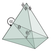
Figure 5: From the dihedral angle relation, we could obtain the internal dihedral angle $\theta$ on a segment. $\alpha$ is the external dihedral angle, while $\theta^{\prime}$ is the angle between normals of the two triangles.

Therefore, $\theta^{\prime}$ is in accordance with the definition of extrinsic curvature in (3), where $K$ is defined as the covariant derivative of the normal $n$ to the hypersurface $\Sigma$. Because of this reason, we define $\theta^{{}^{\prime}}$ as the 2D extrinsic curvature, since in a general curved case, it will inherit the curvature of the 3D manifold.

III.3 Discrete Gauss-Codazzi equation in (2+1) dimension

A simpler but equivalent way to obtain the 3D instrinsic curvature is to use the purely geometrical picture of the discretized manifold. See FIG. 6.

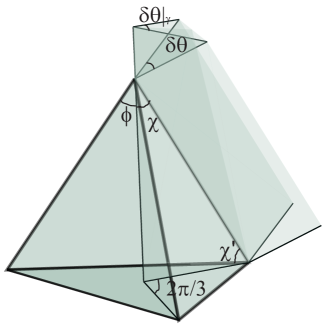
Figure 6: The 3D deficit angle on each segment can be thought as a ’piece of space’ inserted along the hinge. The ’size’ of this ’piece of space’ is described by the deficit angle $\delta\theta,$ which is located on the plane normal to the hinge. The total deficit angle $\delta\Theta$ obtained by adding three rotation in (26), is located in the plane normal to an ’artificial’ hinge in the direction $\hat{k}$, since we use isosceles tetrahedron. Therefore, projecting $\delta\theta$ to this plane, we obtain $\left.\delta\theta\right|_{\gamma}$.

From Figure 6, we obtain the projected 3D intrinsic curvature of each segment on the ’artificial’ segment dual to the total plane of rotation as:

$$\cos^{2}\frac{\left.\delta\theta\right|_{\gamma}}{2}=\frac{\sin^{2}\chi^{\prime}\cos^{2}\frac{\delta\theta}{2}}{1-\cos^{2}\chi^{\prime}\cos^{2}\frac{\delta\theta}{2}}.$$ (29)

Using

$$\vec{J}_{i}=\sin\chi^{\prime}\hat{k}+\cos\chi\hat{r}_{i},$$

we obtain:

$$\left\langle\vec{J}_{i},\vec{J}_{j}\right\rangle=\cos\phi=\sin^{2}\chi^{\prime}+\cos^{2}\chi^{\prime}\cos^{2}\frac{2\pi}{3},$$

or:

$$\cos^{2}\chi^{\prime} = \frac{2}{3}\left(1-\cos\phi\right),$$ (30)

$$\sin^{2}\chi^{\prime} = \frac{1}{3}\left(1+2\cos\phi\right),$$ (31)

since we use isosceles tetrahedron. All the curvatures: 3D intrinsic, 2D intrinsic, and 2D extrinsic curvatures are contained in (29), through:

$$\left.\delta\theta\right|_{\gamma}=\frac{\delta\Theta}{3}=\frac{{}^{3}R}{3},$$ (32)

$$\phi=\frac{2\pi-\delta\phi}{3}=\frac{2\pi-{}^{2}R}{3}$$ (33)

$$\delta\theta=\pi-\left(\theta+\theta^{\prime}\right)=\pi-\left(\arccos\left(\frac{\cos\phi}{1+\cos\phi}\right)+K\right).$$ (34)

Using the half-angle formula and inserting (30)-(34) to (29), we obtain the relation between angles of the discrete Gauss-Codazzi equation for a special discretization using isosceles tetrahedra:

$$1-\cos\left(K+\arccos\left(\frac{\cos\frac{2\pi-{}^{2}R}{3}}{1+\cos\frac{2\pi-{}^{2}R}{3}}\right)\right)=\frac{1+\cos\frac{{}^{3}R}{3}}{1-\frac{1}{3}\left(1-\cos\frac{{}^{3}R}{3}\right)\left(1-\cos\frac{2\pi-{}^{2}R}{3}\right)}.$$ (35)

Together with their planes of rotation: $j$ in (17) for ${}^{2}R$ and $\hat{k}\cdot\bar{\sigma}$ for ${}^{3}R$ (since we use isosceles tetrahedron), (35) is the Gauss-Codazzi equation in plane-angle representation, which contains same amount of information provided by the linear Gauss-Codazzi equation in holonomy representation in (15).

IV Spin network states and 3D loop quantum gravity

IV.1 2-complex and its slice

In this section, we apply the results obtained above to loop quantum gravity (LQG). We will briefly review the quantization of gravity in first order formalism using the loop representation. From the real space representation, we move to the (Hodge) dual space key-8 . (The dual space is introduced in analogy to what is usually done in higher dimension.) In LQG, the fundamental geometrical object is the 2-complex. A 2-complex is a 2-dimensional geometrical object dual to the discrete manifold $M_{\triangle}.$ Let us call the 2-complex as $\star M_{\triangle}$. We can take a slice on a 2-complex, which is a 1-complex called as $\star\Sigma_{\triangle}$, dual to the discrete hypersurface $\Sigma_{\triangle}$ of $M_{\triangle}.$ A 1-complex is a graph consisting oriented lines called links $l$ and points called nodes $n$. The variables attached to the graphs are the variables coming from first order formalism: the holonomy $U_{l}\in SU(2)$ and algebra $J_{l}\in\mathfrak{su(2)}^{*}$ on each links $l$ of the graph. A graph with elements of $SU(2)\times\mathfrak{su(2)}^{*}$ is called a spin network. In the canonical quantization, we promote $\left\{U_{l},J_{l}\right\}$ to operators $\left\{\hat{U}_{l},\hat{J}_{l}\right\}$. The space $SU(2)\times\mathfrak{su(2)}^{*}$ is the phase-space of LQG, and the pair $\left\{\hat{U}_{l},\hat{J}_{l}\right\}$ are the pair conjugate to each other, satisfying a quantized-algebra structure as follow key-3 ; key-8 ; key-11 :

$$\left[\hat{U}_{l},\hat{U}_{l^{\prime}}\right] = 0$$

$$\left[\hat{U}_{l},\hat{J}_{l^{\prime}}^{i}\right] = -\delta_{ll^{\prime}}\bar{\sigma}^{i}\hat{U}_{l}$$

$$\left[\hat{J}_{l}^{i},\hat{J}_{l^{\prime}}^{j}\right] = -\delta_{ll^{\prime}}\varepsilon_{\;k}^{ij}\hat{J}_{l}^{k}.$$

On each node, the gauge invariant condition must be satisfied:

$$\hat{\mathcal{G}}\left|\psi\right\rangle=\sum_{l\in n}\hat{J}_{l}\left|\psi\right\rangle=0.$$

This condition selects an invariant Hilbert space $\mathcal{K}=L_{2}\left[SU(2)^{l}/SU(2)^{n}\right]\ni\left|\psi\right\rangle$ of a closed triangle formed by $\left\{\hat{J}_{1},\hat{J}_{2},\hat{J}_{3}\right\}$ key-3 ; key-8 ; key-11 . As an example for our case, see FIG. 7.

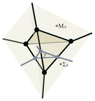
Figure 7: The figure above is a 2-complex dual to the geometric figure in FIG. 1. Suppose we have a 3-dimensional curved manifold $M_{\Delta}$ discretized by four tetrahedron as the first figure above (in flat case it is known as 1-4 Pachner move). Then we take an embedded slice $\Sigma_{\triangle}$ as the surface of one tetrahedron (the dark blue surface discretized by three triangle). Going to the dual space picture, $M_{\Delta}$ is dual to a 2-complex $\star M_{\Delta}$ called as the 3D bubble key-8 (its geometry is defined by black lines and black points), while $\Sigma_{\triangle}$ is dual to a 1-complex $\star\Sigma_{\triangle}$ called as 2D bubble (defined by purple lines and point). Clearly, the 2D bubble $\star\Sigma_{\triangle}$ is embedded on the 3D bubble $\star M_{\Delta}$. The bubble graph define complete curvature of the portion of space.

IV.2 Curvature operators

Given a 2D bubble graph with a phase space variable on each link, we can construct the operators of 3D, 2D intrinsics and 2D extrinsic curvature from these variables.

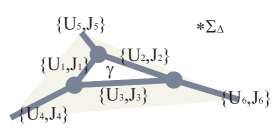
Figure 8: Taking only the slice on the dual space representation, we obtain the spin network $\star\Sigma_{\triangle}.$ $\gamma$ is the loop chosen. Inside $\gamma$ is where the point $p$ located in the real space representation.

We construct these operators using the basic phase-space operators, for example, the angle operator from the phase-space variables key-12 :

$$\hat{\phi}_{i}=\arccos\left(\frac{\left|\hat{J}_{j}\right|^{2}+\left|\hat{J}_{k}\right|^{2}-\left|\hat{J}_{i}\right|^{2}}{2\left|\hat{J}_{j}\right|\left|\hat{J}_{k}\right|}\right),\quad i,j,k\in n.$$

From this angle operator, we obtain the 2D intrinsic curvature along loop $\gamma$ as:

$${}^{2}\hat{R}=2\pi-\sum_{i\subseteq\gamma}\hat{\phi}_{i},$$

which is clearly the deficit angle on a point in the real space representation. See FIG. 8.

The 3D intrinsic curvature can be obtained from the holonomy around a loop. Remember that the direct geometrical interpretation of spacetime can only be obtained from second order formalism, while in LQG, the fundamental variables comes from first order formalism: the holonomy $U$ comes from the curvature 2-form $F$, instead of the Riemannian curvature $R$ (see Section 1). The relation between $F$ and $R$, subjected to the torsionless condition is:

$$R=e\left(F\right),$$ (36)

with $e$ is the local trivialization map between them. Contracting (36) with an infinitesimal area inside the loop (carried by the derivation in Section 1) gives:

$$H=e\left(U\right),\quad U=e^{-1}\left(H\right),$$

since $e$ is a diffeomorphism and must have inverse.

The 3D intrinsic curvature is ${}^{3}R\sim\textrm{tr}H$, with $H$ is the holonomy coming from the contraction of Riemanian curvature $R$ with an infinitesimal area. But since $e$ is a diffeomorphism and trace of the holonomy is invariant under diffeomorphism and gauge transformation, we obtain $\textrm{tr}H=\textrm{tr}U.$ Therefore, we can write the 3D intrinsic curvature operator as:

$${}^{3}\hat{R}=2\arccos\frac{\textrm{tr}\hat{U}_{1}\hat{U}_{2}\hat{U}_{3}}{2}.$$ (37)

The extrinsic curvature operator can be obtained directly from the discrete Gauss-Codazzi equation (35):

$$\hat{K}=\arccos\left(1-\frac{1+\cos\frac{{}^{3}\hat{R}}{3}}{1-\frac{1}{3}\left(1-\cos\frac{{}^{3}\hat{R}}{3}\right)\left(1-\cos\frac{2\pi-{}^{2}\hat{R}}{3}\right)}\right)-\arccos\left(\frac{\cos\frac{2\pi-{}^{2}\hat{R}}{3}}{1+\cos\frac{2\pi-{}^{2}\hat{R}}{3}}\right).$$

IV.3 The semi-classical limit

In this section, we show that the linearity of the relation between $\textrm{tr}\,^{3}H$ and $\textrm{tr}\,^{2}H$ in equation (20) is recovered from the spin network calculation in the semi-classical limit, by dropping the Maslov phase. Let us take a simple spin network illustrated in FIG. 9.

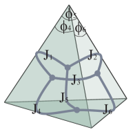
Figure 9: A simple spin network $\star\Sigma_{\Delta}$ (the graph in purple), which will give a geometrical interpretation of a ’fuzzy’ quantum tetrahedron in the semi-classical limit. This spin network can be obtained from the spin network in FIG. 8, by identifying their open links together. In 3D theory, the nodes (purple points) are dual to triangles, and the links (purple lines) are dual to segments.

For simplicity in our calculation, we use a closed graph as an example, but the result is valid for any spin network graph. The vector and covector state of the spin network $\star\Sigma_{\Delta}$ in the algebra representation are:

$$\left|\psi\right\rangle=\sum_{\binom{m_{1}\ldots m_{6}}{n_{1}..n_{6}}}i^{m_{6}m_{3}n_{2}}i^{m_{5}m_{2}n_{1}}i^{m_{4}m_{1}n_{3}}i^{n_{6}n_{5}n_{4}}\left|j_{1}m_{1}n_{1}\ldots j_{6}m_{6}n_{6}\right\rangle,$$ (38)

$$\left\langle\psi\right|=\sum_{\binom{m_{1^{\prime}}\ldots m_{6^{\prime}}}{n_{1^{\prime}}..n_{6^{\prime}}}}i^{m_{6}^{\prime}m_{3}^{\prime}n_{2}^{\prime}}i^{m_{5}^{\prime}m_{2}^{\prime}n_{1}^{\prime}}i^{m_{4}^{\prime}m_{1}^{\prime}n_{3}^{\prime}}i^{n_{6}^{\prime}n_{5}^{\prime}n_{4}^{\prime}}\left\langle j_{1}^{\prime}m_{1}^{\prime}n_{1}^{\prime}\ldots j_{6}^{\prime}m_{6}^{\prime}n_{6}^{\prime}\right|,$$ (39)

with $i$ is the intertwinner attached on the node. See key-8 ; key-11 ; key-13 for a detail explanation about the spin network state. Changing the representation basis using:

$$\left.\left\langle U\right|jmn\right\rangle=D_{mn}^{j}\left(U\right),$$

with $D_{mn}^{j}\left(U\right)$ is the matrix representation of $U\in SU(2)$ in $(2j+1)$-dimension, we can write the vector and covector states in the group representation basis:

$$\left|\psi\right\rangle=\sum_{\binom{m_{1}\ldots m_{6}}{n_{1}..n_{6}}}i^{m_{6}m_{3}n_{2}}i^{m_{5}m_{2}n_{1}}i^{m_{4}m_{1}n_{3}}i^{n_{6}n_{5}n_{4}}\intop dU_{1}..dU_{6}\prod_{i=1}^{6}D_{m_{i}n_{i}}^{j_{i}}\left(U_{i}\right)\left|U_{1}..U_{6}\right\rangle,$$

$$\left\langle\psi\right|=\sum_{\binom{m_{1^{\prime}}\ldots m_{6^{\prime}}}{n_{4^{\prime}}..n_{6^{\prime}}}}i^{m_{6}^{\prime}m_{3}^{\prime}n_{2}^{\prime}}i^{m_{5}^{\prime}m_{2}^{\prime}n_{1}^{\prime}}i^{m_{4}^{\prime}m_{1}^{\prime}n_{3}^{\prime}}i^{n_{6}^{\prime}n_{5}^{\prime}n_{4}^{\prime}}\intop dU_{1}^{\prime}..dU_{6}^{\prime}\prod_{i=1}^{6}D_{m_{i}^{\prime}n_{i}^{\prime}}^{j_{i}^{\prime}}\left(U_{i}^{\prime}\right)\left\langle U_{1}^{\prime}..U_{6}^{\prime}\right|.$$

We choose a specific closed path on spin network $\star\Sigma_{\Delta}$, say, loop $\gamma$, defined by links $\left\{1-2-3\right\}$ (See FIG. 9). The holonomy $U=U_{1}U_{2}U_{3}$ are attached along $\gamma$, therefore we have a well-defined operator related to the 3D intrinsic curvature operator (37) on the loop:

$$\textrm{tr}\,^{3}H=\underset{2\cos\frac{{}^{3}\hat{R}}{2}}{\underbrace{\textrm{tr}U}}=\textrm{tr}\left(U_{1}U_{2}U_{3}\right)=\sum_{m,n}\delta_{mn}D_{mn}^{j}\left(U_{1}U_{2}U_{3}\right).$$ (40)

Since the matrix representation satisfies:

$$\left\langle j,m\right|\hat{D}\left(U_{1}U_{2}U_{3}\right)\left|j,n\right\rangle=D_{mn}^{j}\left(U_{1}U_{2}U_{3}\right)=\sum_{k,l}D_{mk}^{j}\left(U_{1}\right)D_{kl}^{j}\left(U_{2}\right)D_{ln}^{j}\left(U_{3}\right),$$ (41)

we can write

$$\textrm{tr}\,^{3}H=\sum_{k,l,m,n}\delta_{mn}D_{mk}^{j}\left(U_{1}\right)D_{kl}^{j}\left(U_{2}\right)D_{ln}^{j}\left(U_{3}\right).$$ (42)

The geometrical interpretation of the spin-$j$ in (40)-(42) is the measure on the ’artificial’ hinge dual to the plane of rotation inside loop $\gamma.$ See FIG. 6 and Section III C.

Acting $\textrm{tr}\,^{3}H$ with the spin network states gives:

$$\left\langle\psi\right|\textrm{tr}\,^{3}H\left|\psi\right\rangle= \left(\sum_{m_{6},l,m_{3},n_{2},m_{3^{\prime}},n_{2^{\prime}}}i^{m_{6}m_{3}n_{2}}i^{m_{6}m_{3}^{\prime}n_{2}^{\prime}}i^{m_{3}lm_{3}^{\prime}}i^{n_{2}ln_{2}^{\prime}}\right)\left(\sum_{m_{5},k,m_{2},n_{1},m_{2^{\prime}},n_{5^{\prime}}}i^{m_{5}m_{2}n_{1}}i^{m_{5}m_{2}^{\prime}n_{1}^{\prime}}i^{m_{2}km_{2}^{\prime}}i^{n_{1}kn_{1}^{\prime}}\right)\times..$$

$$\;...\times\left(\sum_{m_{4},m,m_{1},n_{3},m_{1^{\prime}},n_{3^{\prime}}}i^{m_{4}m_{1}n_{3}}i^{m_{4}m_{1}^{\prime}n_{3}^{\prime}}i^{n_{3}mn_{3}^{\prime}}i^{m_{1}mm_{1}^{\prime}}\right)\left(\sum_{n_{4}..n_{6}}i^{n_{6}n_{5}n_{4}}i^{n_{6}n_{5}n_{4}}\right),$$

but the first three-terms in the parantheses are only the Wigner 6j-symbols:

$$\left\langle\psi\right|\textrm{tr}\,^{3}H\left|\psi\right\rangle=\underset{\prod_{i=1}^{3}\left\{6j\right\}_{i}}{\underbrace{\left\{\begin{array}[]{ccc}j_{6}&j_{3}&j_{2}\\ j_{3}^{\prime}&j_{2}^{\prime}&j\end{array}\right\}\left\{\begin{array}[]{ccc}j_{5}&j_{2}&j_{1}\\ j_{2}^{\prime}&j_{1}^{\prime}&j\end{array}\right\}\left\{\begin{array}[]{ccc}j_{4}&j_{1}&j_{3}\\ j_{1}^{\prime}&j_{3}^{\prime}&j\end{array}\right\}}}\left(\sum_{n_{4}..n_{6}}i^{n_{6}n_{5}n_{4}}i^{n_{6}n_{5}n_{4}}\right).$$ (43)

We are ready to take the semi-classical limit by setting all the $j_{i}$’s to be large. Using the result proved by Roberts key-14 ; key-15 , for large spin $j,$ the 6j-symbol can be approximated as follow:

$$\left\{6j\right\}=\left\{\begin{array}[]{ccc}j_{1}&j_{2}&j_{3}\\ j_{4}&j_{5}&j_{6}\end{array}\right\}\approx\frac{1}{\sqrt{12\pi\left|V\right|}}\cos\left(\sum_{i=1}^{6}j_{i}\theta_{i}-\frac{\pi}{4}\right),$$

where the six $j_{i}$ constructs a tetrahedron, $\theta_{i}$ are the internal dihedral angle on segment $j_{i},$ and $\left|V\right|$ is the volume of the tetrahedron. The $\frac{\pi}{4}$ term is known as the Maslov phase. Using this result to our case, we obtain:

$$\left\{\begin{array}[]{ccc}j_{6}&j_{3}&j_{2}\\ j_{3}^{\prime}&j_{2}^{\prime}&j\end{array}\right\} \approx\frac{1}{\sqrt{12\pi\left|V\right|}}\cos\left(j_{6}\theta_{6}+j_{3}\theta_{3}+j_{2}\theta_{2}+j_{3}^{\prime}\theta_{3}^{\prime}+j_{2}^{\prime}\theta_{2}^{\prime}+j\theta_{l}-\frac{\pi}{4}\right)$$ (46)

$$\approx\frac{1}{\sqrt{12\pi\left|V\right|}}\cos\left(j_{6}\theta_{6}+2j_{3}\theta_{3}+2j_{2}\theta_{2}+j\theta_{l}-\frac{\pi}{4}\right).$$ (47)

where the last step we use the fact that $j_{i}=j_{i}^{\prime},$ noting that $j_{i}^{\prime}$ comes from the covector state (39). This fact also cause $\theta_{i}=\theta_{i}^{\prime}$. See FIG. 10.

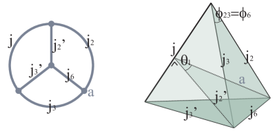
Figure 10: The 6j-symbol $\left\{\begin{array}[]{ccc}j_{6}&j_{3}&j_{2}\\ j_{3}^{\prime}&j_{2}^{\prime}&j\end{array}\right\}$ can be represented using a graph (left), where it can be translated into its dual (right) which is a tetrahedron. Node $a$ on the graph is the triangle $a$ on the tetrahedron. $\theta_{l}$ is the dihedral angle on $j.$

Remember that $j$ is the measure on the ’artificial’ hinge inside loop $\gamma$, in other words, the spin number $j$ is the ’length’ of the artificial hinge. Along this artificial hinge, there is a point $p$ where the 2D deficit angle is located. Taking $j_{i}\ggg j,$ we have:

$$\theta_{6}\approx 0,\>\theta_{3}\approx\frac{\pi}{2},\>\theta_{2}\approx\frac{\pi}{2},\>\theta_{l}\approx\phi_{23}=\phi_{6},$$

See FIG. 10. Using this approximation, (47) becomes:

$$\left\{\begin{array}[]{ccc}j_{6}&j_{3}&j_{2}\\ j_{3}^{\prime}&j_{2}^{\prime}&j\end{array}\right\}\approx\frac{1}{\sqrt{12\pi\left|V_{1}\left(j_{6},j_{3},j_{2},j\right)\right|}}\cos\left(\left(j_{3}+j_{2}\right)\pi+j\phi_{6}-\frac{\pi}{4}\right).$$

Doing the same way for the other two 6j-symbols, we obtain:

$$\left\{\begin{array}[]{ccc}j_{5}&j_{2}&j_{1}\\ j_{2}^{\prime}&j_{1}^{\prime}&j\end{array}\right\}\approx\frac{1}{\sqrt{12\pi\left|V_{2}\left(j_{5},j_{2},j_{1},j\right)\right|}}\cos\left(\left(j_{2}+j_{1}\right)\pi+j\phi_{5}-\frac{\pi}{4}\right),$$

$$\left\{\begin{array}[]{ccc}j_{4}&j_{1}&j_{3}\\ j_{1}^{\prime}&j_{3}^{\prime}&j\end{array}\right\}\approx\frac{1}{\sqrt{12\pi\left|V_{3}\left(j_{4},j_{1},j_{3},j\right)\right|}}\cos\left(\left(j_{1}+j_{3}\right)\pi+j\phi_{4}-\frac{\pi}{4}\right).$$

By writing the cosine function using the Euler formula:

$$\cos x = \frac{1}{2}\left(\exp ix+\exp-ix\right),$$

we can write the products of the three 6j-symbols as:

$$\prod_{i=1}^{3}\left\{6j\right\}_{i} \approx \frac{1}{4}\frac{1}{12\pi\sqrt{12\pi\left|V_{1}\right|\left|V_{2}\right|\left|V_{3}\right|}}\times\left(\>\cos\left(2\left(j_{1}+j_{2}+j_{3}\right)\pi+j\left(\phi_{4}+\phi_{5}+\phi_{6}\right)-\frac{3\pi}{4}\right)+...\right.$$ (48)

$$\qquad...+\cos\left(2j_{3}\pi+j\left(\phi_{4}-\phi_{5}+\phi_{6}\right)-\frac{\pi}{4}\right)+\cos\left(2j_{2}\pi+j\left(-\phi_{4}+\phi_{5}+\phi_{6}\right)-\frac{\pi}{4}\right)+...$$

$$\qquad...+\left.\cos\left(2j_{1}\pi+j\left(\phi_{4}+\phi_{5}-\phi_{6}\right)-\frac{\pi}{4}\right)\,\right).$$

From this point, we take the sum of $j_{1}+j_{2}+j_{3}$ to be an integer/natural number (we discard the half-integer possibility) and choose the spin number $j=1,$ then we could write:

$$\prod_{i=1}^{3}\left\{6j\right\}_{i} \approx\frac{1}{4}\frac{1}{12\pi\sqrt{12\pi\left|V_{1}\right|\left|V_{2}\right|\left|V_{3}\right|}}\>\cos\left(\delta\phi-\frac{3\pi}{4}\right)+\mathcal{O},$$ (49)

where we denoted the remaining terms by $\mathcal{O}$ and using $\phi_{4}+\phi_{5}+\phi_{6}=2\pi-\delta\phi$ (see FIG. 9). Inserting (49) to (43), we obtain:

$$\left\langle\cos\frac{{}^{3}\hat{R}}{2}\right\rangle \sim\left\langle\cos\left({}^{2}\hat{R}-\frac{3\pi}{4}\right)\right\rangle.$$

The linearity relation (20) can be recovered by dropping the Maslov phase:

$$\left\langle\textrm{tr}\,^{3}H\right\rangle \sim\left\langle\textrm{tr}\,^{2}H\right\rangle.$$

An important point is we have a freedom to choose the spin number $j,$ since this spin number comes from (40), which is the dimension of the $SU(2)$ representation. If we set $j=0,$ then, the volume of the 6j tetrahedra $\left|V_{i}\right|$ will be zero and relation (48) will diverge, given any $j_{i}^{\prime}$s. But since the range of spin $j$ is $j\geq\frac{1}{2}$, with $j$ multiple of half, then the spin number $j$ acts as an ultraviolet cut-off which prevents relation (48) from divergence.

V Conclusion

We have obtained the Gauss-Codazzi equation for a discrete (2+1)-dimensional manifold, discretized by isosceles tetrahedra. We have studied the definition of extrinsic curvature in the discretized context. With definitions of the 3-dimensional intrinsic, 2-dimensional intrinsic, and 2-dimensional extrinsic curvature in the discrete picture, we have promoted them to curvature operators, acting on the spin network states of (2+1)-dimensional loop quantum gravity. In the semi classical limit, we have shown that the linearity between $\textrm{tr}\,^{3}H$ and $\textrm{tr}\,^{2}H$ in equation (20) is recovered in the spin network calculation, by dropping the Maslov phase. There exist a natural ultraviolet cut-off which prevents the discrete Gauss-Codazzi equation from divergences in the semi-classical limit.

References

- (1) S. M. Carroll. Spacetime and geometry: An introduction to general relativity. San Francisco, CA, USA. Addison-Wesley. ISBN 0-8053-8732-3. 2004.
- (2) T. Regge, R. M. Williams. Discrete structures in gravity. J. Math. Phys. 41, 3964 (2000). arXiv:gr-qc/0012035v1.
- (3) P. Don, S. Speziale. Introductory lectures to loop quantum gravity. (2010). arXiv:gr-qc/1007.0402.
- (4) J. W. Barrett and I. Naish-Guzman. The Ponzano-Regge model. Class. Quant. Grav. 26: 155014 (2009). arXiv:gr-qc/0803.3319.
- (5) T. Regge. General relativity without coordinates. Nuovo Cim. 19 (1961) 558. http://www.signalscience.net/files/Regge.pdf.
- (6) R. Arnowitt, S. Deser, C. Misner. Dynamical Structure and Definition of Energy in General Relativity. Phys. Rev. 116 (5): 1322-1330. (1959).
- (7) C. Rovelli, F. Vidotto. Covariant Loop Quantum Gravity: An Elementary Introduction to Quantum Gravity and Spinfoam Theory. UK. Cambridge University Press. ISBN 978-1-107-06962-6. 2015.
- (8) J. C. Baez, J. P. Muniain. Gauge Fields, Knots, and Gravity. Series on Knots and Everything: vol 4. World Scientific Pub Co Ltd. ISBN 9789810220341. 1994.
- (9) H. W. Hamber. Quantum Gravitation: The Feynman Path Integral Approach. Springer-Verlag. ISBN 978-3-540-85292-6. 2009.
- (10) B. C. Hall. An Elementary Introduction to Groups and Representations. Graduate Texts in Mathematics 222 (2003). Springer-Verlag. arXiv:math-ph/0005032v1.
- (11) C. Rovelli. Zakopane lectures on loop gravity. (2011). arXiv:gr-qc/1102.3660.
- (12) M. Seifert. Angle and Volume Studies in Quantized Space. arXiv:gr-qc/0108047.
- (13) S. A. Major. A Spin Network Primer. Am. J. Phys. 67 (1999) 972-980. arXiv:gr-qc/9905020.
- (14) J. Roberts. Classical 6j-symbols and the tetrahedron. Geom. Topol. 3 (1999). arXiv:math-ph/9812013.
- (15) G. Ponzano and T. Regge. Semiclassical Limit of Racah Coefficients. Spectroscopy and Group Theoretical Methods in Physics. Amsterdam. pp. 1-58 (1968).