The Infrared Massive Stellar Content of M83 ,

Abstract

Aims. We present an analysis of archival Spitzer images and new ground-based and Hubble Space Telescope (HST) near-infrared (IR) and optical images of the field of M83 with the goal of identifying rare, dusty, evolved massive stars.

Methods. We present point source catalogs consisting of 3778 objects from Spitzer Infrared Array Camera (IRAC) Band 1 (3.6 $\mu$m) and Band 2 (4.5 $\mu$m), and 975 objects identified in Magellan 6.5m FourStar near-IR $J$ and $K_{\rm s}$ images. A combined catalog of coordinate matched near- and mid-IR point sources yields 221 objects in the field of M83.

Results. We find 49 strong candidates for massive stars which are very promising objects for spectroscopic follow-up. Based on their location in a $B-V$ versus $V-I$ diagram, we expect at least 24, or roughly 50%, to be confirmed as red supergiants.

1 Introduction

Massive stars are of prime importance in astrophysics. The consequences of their birth and evolution have profound ramifications for galaxy evolution. Throughout their lives, their physical characteristics shape and mold their immediate environment via intense radiation fields and strong winds. Many massive stars expire as supernovae (SNe), thus affecting subsequent star formation and the chemical enrichment of galaxies, their interstellar media, and the intergalactic medium. Predicting the evolution of a massive star relies heavily upon the mass loss experienced by a star over the course of its life.

Mass loss in massive stars ($M\gtrsim 8M_{\odot}$), particularly in the late stages of evolution, is poorly understood (see the recent review by Smith 2014). Wind mass loss rates of massive stars on the main sequence, once thought to be a major contributor to massive star mass loss, are now being revised to be 2 to 3 times lower than previous estimates based on observations in the ultraviolet and optical (see Crowther et al. 2002; Repolust et al. 2004; Puls et al. 2006, for example) as well as in the X-ray (Cohen et al. 2011). Episodic and eruptive mass loss in evolved massive stars must therefore be more important than previously thought.

Understanding mass loss via observations of Galactic massive stars is difficult. Massive stars are rare and are formed in regions along the Galactic plane where extinction can be patchy and very high. For example, Ramírez Alegría et al. (2012) estimate visual extinctions up to 21.5 mag for members of the young massive stellar cluster Masgomas-1 at a distance of $\sim$3.5 kpc. In order to observe massive stars at large distances in the Milky Way, it becomes necessary to observe them in the infrared (IR). By far the best efforts to discover new Galactic massive stars exhibiting heavy mass loss have been most successful using Spitzer 24 $\mu$m observations that revealed circumstellar shells of ejected material surrounding massive evolved stars (e.g. Gvaramadze et al. 2010; Wachter et al. 2010). In order to form a more complete census, however, we must look outside our own Galaxy.

The consequences of late evolutionary stage mass loss for lower mass stars may be seen in the progenitors of some supernovae. One specific example is SN 2012aw, a type IIP event in the galaxy M95 (Fagotti et al. 2012). Pre-explosion mass loss is likely responsible for the dusty circumstellar material (CSM) seen as a significant visual extinction around the red supergiant (RSG) progenitor that has a mass at the high end of the range for type IIP SN progenitors (Fraser et al. 2012; Van Dyk et al. 2012).

The situation concerning mass loss in more massive stars is uncertain. SN 2009ip was initially mistakenly identified as a SN (Maza et al. 2009) based on its initial rise in brightness. However, it never reached typical SNe magnitudes, and was eventually understood to be an object undergoing a luminous blue variable (LBV) eruption (Berger et al. 2009; Miller et al. 2009). SN 2009ip also experienced a similar outburst in 2010, followed by a brighter event in 2012. The jury is still out concerning whether SN 2009ip is a true SN (Mauerhan et al. 2013; Smith 2014; Mauerhan et al. 2014; Graham et al. 2014) or an imposter (Pastorello et al. 2013; Margutti et al. 2014; Fraser et al. 2015), but poorly understood mass loss events have clearly played a vital role in shaping the late stages of evolution for this $50-80M_{\odot}$ star. The specifics of episodic and eruptive mass loss mechanisms in both the higher mass ($\gtrsim 30M_{\odot}$, Humphreys & Davidson 1994; Humphreys et al. 2014) and lower mass regimes (RSGs with masses $\lesssim 30M_{\odot}$, Smith 2014) remain unknown. While the case of SN 2009ip is rare, discovering and cataloging all massive stars with mass loss is a tractable investigation.

Mass loss in massive stars can reveal itself via an IR excess in different ways depending on the type and mass of the star. In a recent study of luminous and variable stars in M31 and M33, Humphreys et al. (2014) found that LBVs had no hot or warm dust evident in the IR. Fe ii emission stars have an IR excess attributed to circumstellar dust and nebulosity, both of which are indicative of mass loss. Meanwhile, only some A-F spectral type supergiants show IR evidence of mass loss, possibly because some are post-RSG objects, while others are still evolving to the red on the Hertzsprung-Russel (HR) diagram. For redder objects (RSGs), mass loss is seen as thermal-IR excess from hot dust and molecular emission (Smith 2014), and masers in the extreme cases (Habing 1996).

Work categorizing the massive stellar content of nearby galaxies in the IR with Spitzer began with the Large Magellanic Cloud (LMC; Blum et al. 2006; Bonanos et al. 2009), Small Magellanic Cloud (SMC; Bonanos et al. 2010) and M33 (Thompson et al. 2009). Bonanos et al. (2009, 2010) laid the foundation for differentiating the types of massive stars by looking at objects with previously known spectral classifications in the LMC and SMC. Thompson et al. (2009) focused on the dust-enshrouded massive stars in M33 identifying several candidates as extreme asymptotic giant branch (EAGB) stars that exhibited very red colors from Spitzer InfraRed Array Camera (IRAC) Band 1 3.6 $\mu$m and Band 2 4.5 $\mu$m observations, and are likely similar to the progenitor of transients like SN 2008S (Prieto et al. 2008). Khan et al. (2010) extended this effort to the nearby galaxies NGC 6946, M33, NGC 300, and M81. Of particular interest was the identification of the brightest mid-IR point source in M33, dubbed Object X (Khan et al. 2011), a likely binary system composed of a massive O star and a dust enshrouded red supergiant (Mikołajewska et al. 2015). A similar search was also applied to look for $\eta$ Car-like objects in NGC 6822, M33, NGC 300, NGC 2403, M81, NGC 247 and NGC 7793 (Khan et al. 2013). Britavskiy et al. (2014) used Spitzer photometry to select bright candidates in the Local Group dIrr galaxies IC 1613 and Sextans A, and their follow-up spectroscopy discovered five new RSGs and one yellow hypergiant candidate.

We aim to continue to characterize the massive stellar content of nearby galaxies with high star formation rates starting with M83. M83 lies outside of the Local Group at a distance of $\sim$4.8 Mpc ($\mu\sim 28.4$ mag, Herrmann et al. 2008; Radburn-Smith et al. 2011). It is a face-on galaxy classified as SAB(s)c (de Vaucouleurs et al. 1991) with the fifth-highest H$\alpha$ luminosity in the local 11 Mpc³ volume (log $L_{\rm H\alpha}$ = 41.25, Kennicutt et al. 2008). The star formation rate for a galaxy is directly proportional to its H$\alpha$ luminosity (Murphy et al. 2011). M83 has also been host to six historical SNe, five of which have been identified as massive star or core-collapse: the Type IIP SN 1923A (Lampland 1923; Rosa & Richter 1988), the unclassified SN 1945B (Liller 1990), the Type II SN 1950B (Haro & Shapley 1950; Weiler et al. 1986), another Type II SN1957D (Kowal & Sargent 1971; Weiler et al. 1986), the Type IIP SN 1968L (Bennett 1968; Barbon et al. 1979), and the Type Ib SN 1983N (Thompson et al. 1983; Porter & Filippenko 1987). The high H$\alpha$ luminosity coupled with the copious amount of historical SNe and SN remnants (Blair et al. 2012, 2014) imply that M83 has a large population of massive young stars. These stars evolve relatively quickly, meaning there may also be a large number of dusty evolved massive stars that are prominent in the high-quality Spitzer archival images. We also supplement Spitzer data with ground-based near-IR and Hubble Space Telescope (HST) Wide Field Camera 3 (WFC3) observations in order to investigate the massive stellar content of M83.

Kim et al. (2012) studied the stellar content of select regions of M83 with a subset of the WFC3 data used here and came to the conclusion that young stars are more likely to be found in concentrated aggregates along spiral arms. Larsen (1999) reached a similar conclusion, noting that highly crowded clusters are less than 10 Myr old, roughly the expected age for RSGs of masses similar to that of the progenitor of SN 2012aw. Also, Chandar et al. (2010), using HST observations, noted that M83 contained a large number of clusters with $M>10^{3}M_{\odot}$ and $\tau<10^{7}\leavevmode\nobreak\ yr$. We therefore focus on methods attempting to find massive star candidates that are demonstrably separate in the data from cluster candidates. We also target the spiral arm regions of M83, in order to investigate the youngest stellar populations.

Section 2 describes the observations and data reduction, with some initial analysis. Section 3 describes the combined catalog between data sets from section 2, and our methods for selecting massive stars from the data. In section 4, we compare our method of selecting evolved massive stars to other methods of photometric selection and present conclusions in section 5.

2 Observations and Data Reduction

2.1 Spitzer Observations

We extracted the mosaic image of M83 from the Local Volume Legacy Survey (LVL, Dale et al. 2009) in all four of the IRAC bands. The final image analyzed here covers an area of 15$\arcmin$ $\times$ 15$\arcmin$ with a pixel scale of $0\aas@@fstack{\prime\prime}75$ pix^-1 centered on the nucleus of M83 (J2000.0: $\alpha=$13:37:00.9, $\delta=-$29:51:56).

Initial point source lists in Spitzer IRAC 3.6 $\mu$m (Band 1) and 4.5 $\mu$m (Band 2) bands were extracted using the IRAF implementations of the DAOPHOT (Stetson 1987, 1992) suite of programs. A point-spread function (PSF) was built for each bandpass from bright, isolated stars. Aperture photometry of the PSF stars was converted to the Vega system using the aperture corrections and zero-point fluxes given in the IRAC Instrument Handbook. PSF magnitudes for the entire set of point sources were then calibrated by applying the offset between PSF magnitudes and corrected aperture magnitudes for the PSF stars. The coordinates for point sources in the 3.6 $\mu$m list were checked against those in the 4.5 $\mu$m list using J. D. Smith’s IDL code match_2d.pro with a half pixel search radius ($0\aas@@fstack{\prime\prime}375$). Positional coordinates were derived from the World Coordinate System (WCS) information contained in the header of the archival LVL image for the 3.6 $\mu$m frame.

To eliminate the possibility of including foreground or other previously identified objects, we checked the positions of candidates in our list against a number of catalogs. Mimicking the method used to match sources between the 3.6 $\mu$m and 4.5 $\mu$m bands, we compared our candidate positions to those in the PPMXL catalog (Roeser et al. 2010), discarding 73 candidates having both a position match, and a proper motion in either right ascension or declination of $>15$ mas yr^-1 (uncertainties in proper motion measurements were on the order of 10 mas). Larsen (1999) studied young massive star clusters in M83, publishing a catalog of 149 clusters. Using the same half pixel search criteria, we found matches to 5 of the Larsen (1999) clusters, and removed them from further analysis. We also checked the cluster list from a study of the central region of M83 by Harris et al. (2001), but found no matches. Herrmann & Ciardullo (2009) list 241 photometrically identified planetary nebulae in M83 from their investigation into the mass-to-light ratio of spiral galaxy disks. A coordinate check against this list resulted in no matches with our candidates. In a reanalysis of European Southern Observatory (ESO) Very Large Telescope (VLT) imaging data covering one $6\aas@@fstack{\prime}8$ $\times$ $6\aas@@fstack{\prime}8$ field in M83, Bonanos & Stanek (2003) discovered 112 Cepheid variables, none of which matched the coordinates of any of our candidates. The supernova remnant population of M83 has been studied in some detail. We compared Spitzer candidates against the object lists in Blair et al. (2012), rejecting 3 objects, and the list of new objects in Blair et al. (2014), finding no matches.

The final 3778 objects in M83 are included in Table 1. The positions of sources in RA and Dec are given in degrees in the first two columns of the table. Based on comparison with positions of 2MASS stars in the observed field, we estimate the astrometry to be accurate to about $0\aas@@fstack{\prime\prime}3$. The remaining columns are made of pairs: the source’s photometry in a bandpass followed by the uncertainty in the measurement. The columns start at the lowest wavelength, with $J$, and continue with $K_{\rm s}$ (described in §2.2 for the near-IR), 3.6 $\mu$m, 4.5 $\mu$m, 5.8 $\mu$m, and 8.0 $\mu$m (described in §3.1). Sources with no detection in a particular bandpass are left with a blank entry. Some sources were only detected in the near-IR or mid-IR and thus only have measurements in $J$ and $K_{\rm s}$ or 3.6 $\mu$m and 4.5 $\mu$m.

We estimated the photometric completeness of the list in a method similar to Bibby & Crowther (2012). We placed detected sources in 0.25 mag bins and fit a power law to the bright end of this distribution. A completeness level limit of 100% is assumed to be where this distribution begins to drop from this power law. The 100% completeness magnitudes are therefore estimated to be $[3.6]\approx 18.3$ mag and $[4.5]\approx 17.5$ mag. These limits correspond to absolute magnitudes of M${}_{[3.6]}\approx$ –10.1 mag and M${}_{[4.5]}\approx$ –10.9 mag using our assumed distance modulus of $\mu\approx 28.4$ mag. Therefore, we are only able to completely sample the most luminous massive stars in these bands.

2.2 FourStar Observations

Observations of M83 were made in $J$ and $K_{\rm s}$ with the FourStar instrument (Persson et al. 2013) attached to the 6.5m Baade Magellan Telescope at Las Campanas Observatory, on UT date 2014 Jan 2. Data reduction was performed with the FSRED package courtesy of A. Monson. The resulting $J$-band mosaic (MJD=56659.31938) was constructed from 7 dithered exposures yielding a maximum exposure time of 335 seconds, while the corresponding $K_{\rm s}$ mosaic (MJD=56659.33165) was the combination of 10 frames giving a maximum exposure time of 582 seconds. Astrometric calibration employed SWarp (Bertin et al. 2002) software and stars from the 2MASS (Skrutskie et al. 2006) catalog. The final images have a field of view of 11$\arcmin$ $\times$ 11$\arcmin$ centered on the nucleus of M83 with a pixel scale of $0\aas@@fstack{\prime\prime}16$ pix^-1.

Photometry for the $J$ and $K_{\rm s}$ bands was conducted in the same fashion as for the Spitzer data. The PSF varied across the four CCDs making up the FourStar instrument, so several PSF stars in each quadrant of the final mosaic were selected. The PSF stars were chosen from the 2MASS catalog and used for both aperture correction and photometric calibration. Because the photometric standard stars were on the same frame as the candidate objects, the transformation equations simplified to a zero-point for each band and color term between the two bands. The computation of transformed magnitudes thus required a source to have a measurement in both the $J$ and $K_{\rm s}$ bands within a matching radius of 2 pixels corresponding to $\sim 0\aas@@fstack{\prime\prime}32$. The 2MASS stars in each bandpass were also subjected to the same transformation, and the comparison of our measured values and those published in the 2MASS catalog are shown in Table 2. The average difference in the $J$-band is $0.047\pm 0.039$ mag, while the average difference for the $(J-K_{\rm s})$ color is $0.056\pm 0.045$ mag. The average difference in $J$ is nearly insignificant, however, the similar difference in the $(J-K_{\rm s})$ color may indicate some systematics with the $J$-band measurements.

Artificial star tests were used to estimate the photometric uncertainty of a measurement similar to the method employed by Grammer & Humphreys (2013). Using the PSF constructed for each bandpass image, we added one thousand artificial stars (a number roughly equal to the total number of point source detections matched between bands) to each frame via the ADDSTAR routine in the DAOPHOT package. We then performed photometry on these targets in the same manner used on the point source candidate list and repeated this process three times. We computed the root-mean-square (rms) of the differences between input and output magnitudes for 0.2 mag bins. This rms difference was then added in quadrature with measurement uncertainties from ALLSTAR falling into that particular bin, to make the final estimate of measurement uncertainty. It should be noted that this rms difference was typically very close in value to the uncertainty estimates from ALLSTAR. The final point source list of 975 objects are included in Table 1. Sources detected in the near-IR are sorted by RA in column 1, with column 2 listing the declination, both in degrees. Again, from comparison with 2MASS sources, we estimate that the FourStar astrometry is accurate to roughly $0\aas@@fstack{\prime\prime}3$. Columns 4 through 7 correspond to $J$ magnitude and measurement uncertainty, and $K_{\rm s}$ magnitude and measurement uncertainty for sources detected in the near-IR. For sources with no $J$ and $K_{\rm s}$ measurements these columns are left blank. We did not correct the point source photometry for foreground Galactic extinction. However, for completeness, the current best estimate using the Schlafly & Finkbeiner (2011) infrared-based dust map gives 0.047 and 0.020 mag in $J$ and $K_{\rm s}$, respectively.

Using the same method as described in §2.1, we found the 100% completeness levels to be 18.0 mag (M${}_{J}\approx$ –10.4) in $J$ and 16.6 mag (M${}_{K_{\rm s}}\approx$ –11.8) in $K_{\rm s}$.

2.3 $HST$ WFC3 Observations

Blair et al. (2014) studied supernova remnants in M83 with seven fields of Hubble Space Telescope (HST) Wide Field Camera 3 (WFC3) observations in multiple bandpasses. Two fields come from the Early Release Science Program (ID 11360; R. O’Connell, PI) with the remaining five coming from the cycle 19 HST General Observer program 12513 (W. Blair, PI). These seven fields cover the majority of the bright disk region of M83. For the reduction and discussions concerning the photometry of these data, we direct the reader to Blair et al. (2014, and references therein). We specifically used the imaging and photometry in the F336W (Johnson $U$), F438W (Johnson $B$), F555W (Johnson $V$) or F547M (Strömgren $y$, easily converted to Johnson $V$), and F814W (Johnson $I$) bands. The quality of the astrometry for the $HST$ data are better than $0\aas@@fstack{\prime\prime}1$ (Blair et al. 2014).

3 Results

3.1 Combined Catalog of Point Sources

In order to characterize the point sources, sources detected in both the near-IR and mid-IR were matched by position as described above. Final coordinates were adopted from the shortest wavelength, $J$, owing to the band having the better spatial resolution compared to longer wavelength bands. To supplement these measurements, aperture photometry using the IRAF task APPHOT/PHOT was performed on the remaining IRAC bands, 5.8 $\mu$m and 8.0 $\mu$m at the pixel positions of sources having $J$, $K_{\rm s}$, 3.6 $\mu$m and 4.5 $\mu$m photometry. The aperture photometry in these two bands was calibrated in the same way as described for the PSF stars in the 3.6 $\mu$m and 4.5 $\mu$m bands in the previous section, with appropriate constants applied from the IRAC instrument handbook.

This near- and mid-IR combined catalog of 221 point sources in M83 is presented in Table 1.

3.2 Candidate Massive Star Collection

Identifying massive star candidates among our point source catalog presents several challenges. For example, the average FWHM of objects in the 3.6 $\mu$m band is $\sim 1\aas@@fstack{\prime\prime}7$, which corresponds to 40 pc at the 4.8 Mpc distance to M83. Thus, virtually all the clusters identified in Larsen (1999) will be unresolved on ground-based images, leaving open the possibility of confusing massive stars with compact clusters or unresolved associations. We also expect contamination from foreground Milky Way halo objects like M-dwarfs, and background galaxies. One way to overcome this limitation is to compare the location of objects on various color-magnitude diagrams (CMDs) and other photometric diagnostic plots. Another way to address this issue is to use higher resolution Hubble images, as employed in the current paper.

3.2.1 Mid-IR Selection Criteria

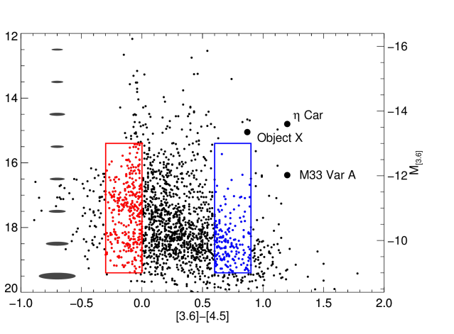
Figure 2: Color-magnitude diagram (CMD) for M83 based on Spitzer IRAC Bands 1 and 2 photometry. Regions empirically known to contain red supergiants (RSGs) and supergiant Be stars (sgB[e]) in Bonanos et al. (2009, 2010) are outlined with red and blue boxes, respectively. Objects that lie within those regions are plotted with red and blue points. On the left side of the plot are shown the average 1$\sigma$ uncertainty ellipses for stars in 1 mag bins for the [3.6] photometry and the [3.6]–[4.5] color. For reference, also plotted are the locations of the prominent evolved massive stars $\eta$ Car (Humphreys & Davidson 1994), M33 Variable A (Humphreys et al. 2006), and Object X (Khan et al. 2010) when placed at the distance ($\sim$4.8 Mpc) of M83.

We applied mid-IR criteria to select massive stars from our sample following the Spitzer Space Telescope Legacy Survey known as “Surveying the Agents of a Galaxy’s Evolution” (SAGE) studied both the LMC (Meixner et al. 2006) and SMC (SAGE-SMC; Gordon et al. 2011) allowing a characterization of the IR properties of the massive stellar content of both galaxies (Bonanos et al. 2009, 2010). In both the LMC (Bonanos et al. 2009) and SMC (Bonanos et al. 2010), massive, evolved stars with previously known spectral types were shown to group in certain regions of the [3.6] versus [3.6]–[4.5] CMD, thanks to the well-studied nature of the brightest stars of these nearby galaxies. Specifically, looking at Figure 2 of both Bonanos et al. (2009) and Bonanos et al. (2010), RSGs are clumped in a region where $-0.3<[3.6]-[4.5]<0.0$ and $-13.0<M_{[3.6]}<-9$, while supergiant Be (sgB[e]) stars are located in a band further to the red, with [3.6]$-$[4.5] between 0.6 and 0.9 and $-13<M_{[3.6]}<-9$. RSGs appear “blue” owing to the suppression of flux in [4.5] from the CO and CO₂ molecular bandheads (Verhoelst et al. 2009). LBVs occupy the [3.6]$-$[4.5] color space between these two groups. There are always exceptions to these generalizations, and one concern may be that the cuts for RSGs may not include stars with dusty envelopes. There is evidence that these photometric cuts are leaving out RSG. For example, in Britavskiy et al. (2014), the RSG IC 1613 1 was originally thought to be an LBV based on its color: [3.6]$-$[4.5]$=0.67$. Follow up spectroscopy, however, revealed it to be an early M supergiant.

Figure 2 shows the [3.6] versus [3.6]$-$[4.5] CMD of point sources from Table 1. Sources are plotted as black dots except for the two regions empirically shown to contain RSGs and sgB[e] stars as discussed above. The RSG region is outlined in a red box, and point sources are shown with red dots, while the sgB[e] region follows the same prescription, but with the color blue. Applying these regional criteria for massive star candidates yields 638 RSGs and 363 sgB[e] candidate stars. Also plotted in Figure 2 are prominent massive stars from the literature: $\eta$ Car (Humphreys & Davidson 1994), M33 Variable A (Humphreys et al. 2006), and Object X (Khan et al. 2011). To represent the accuracy of the photometry, we have plotted ellipses on the left side showing the typical uncertainties in [3.6] and [3.6]$-$[4.5] for each one magnitude bin.

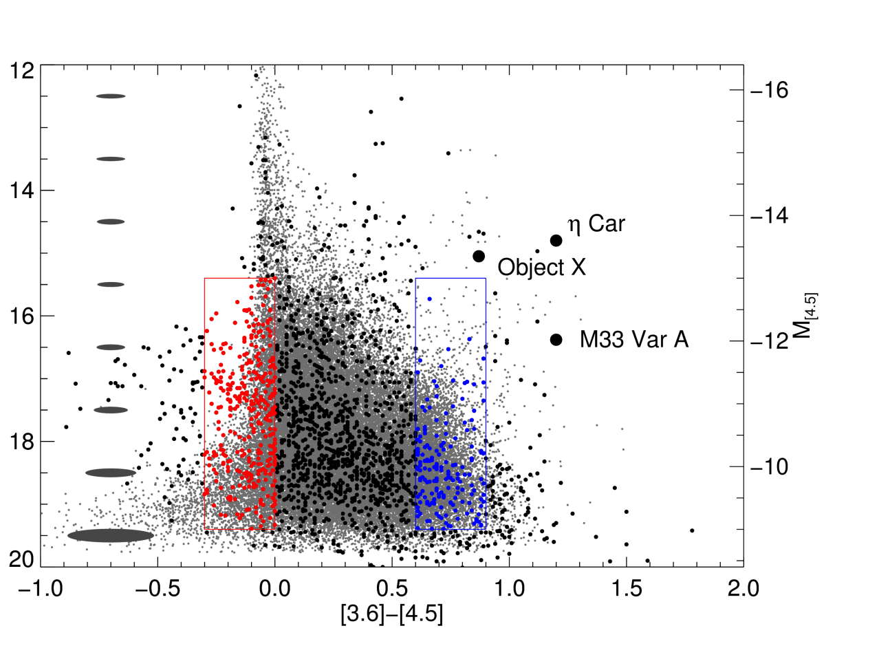
Figure 3: This figure is the same as Figure 2 but includes grey points from the Spitzer Deep Wide Field Survey representing the expected regions of contamination from non-M83 sources. Note that only the more luminous and bluer RSG candidates lie distinctly outside the contaminated region. For reference, also plotted are the locations of the prominent evolved massive stars $\eta$ Car (Humphreys & Davidson 1994), M33 Variable A (Humphreys et al. 2006), Object X (Khan et al. 2011), when placed at the distance ($\sim$4.8 Mpc) of M83.

One major difference between the LMC and SMC versus M83 is that background extragalactic sources become more numerous in the mid-IR CMD at the distance of M83. Ashby et al. (2009) showed that for the Spitzer Deep, Wide-Field Survey (SDWFS), galaxies make up most of their detections. This is especially true past $[3.6]>16$ mag, where many of our massive star candidates exist. We determined the approximate contamination by extracting 42,465 sources from the final version of the SDWFS catalog (Kozłowski et al. 2010) from a randomly selected one square degree area. These are plotted in Figure 3 as small grey dots. Figure 3 is the same as Figure 2 except it also shows the possible regions of contamination by background sources from the SDWFS catalog. This is not entirely representative of the expected contamination in the field of M83, as it contains all objects within a one square degree region while the analyzed M83 Spitzer image covers only 15$\arcmin$ $\times$ 15$\arcmin$.

To further explore the background contamination, the same selection criteria used to find massive star candidates in M83 were applied to the sample from the SDWFS, yielding 4309 objects in the RSG area and 5348 objects in the sgB[e] region. We then scaled these numbers for the area encompassed by the extracted Spitzer image of M83, 15$\arcmin$ $\times$ 15$\arcmin$ or 0.0625 square degrees. The final estimates for contamination are 270 (42%) in the RSG region, leaving 368 RSG candidates and 335 (92%) in the sgB[e] region, with only 28 objects not likely to be background contaminants. Khan et al. (2013) used similar methods to estimate their contamination, finding it to be much less for galaxies closer to the Milky Way. In a study of the asymptotic giant branch (AGB) and super-AGB (SAGB) population of the LMC, Dell’Agli et al. (2014) showed that the most massive ($6-8M_{\odot}$) AGBs, the OH/IR stars, exist at luminosities above the classic limit for AGBs of $L\sim 5\times 10^{4}L_{\odot}$ or $M_{bol}=-7.1$ mag. The AGB region outlined in Khan et al. (2010) lies in a slightly reddened part of the CMD, redward of [3.6]$-$[4.5]$=$0.1 mag and where $M_{\rm[3.6]}<-10$ mag. However, given the photometric uncertainties at the distance of M83, there is the possibility that some photometrically identified evolved massive star candidates may actually be the most massive and most luminous AGB/SAGB stars.

The strongest massive star candidates from the Spitzer photometry are those objects that lie outside the background contaminated region shown in Figure 3. These include a number of objects that may be very red objects [3.6]$-$[4.5] $>1.5$ mag or objects with colors bluer than RSGs. The strongest RSG candidates lie in the region bounded by $-0.3<$ [3.6]$-$[4.5] $<-0.1$ mag for 15.4 $<$ [3.6] $<$ 16.5 mag and in the bounding box above the line connecting the two points of [3.6] = 16.5 mag and [3.6]$-$[4.5]$=-0.1$ mag with [3.6] = 18.0 mag and [3.6]$-$[4.5]$=-0.3$ mag. It should be noted that photometric uncertainties may shift some candidates into and other objects out of this region. Regardless, these criteria resulted in the identification of 118 candidates from the Spitzer photometry. Further refinement was made via plotting the positions of these candidates over an image of the galaxy. The extent of the images used in this analysis (15$\arcmin$ $\times$ 15$\arcmin$) goes well beyond the disk light of M83. While massive stars exist in the outer regions of M83, they will be more numerous particularly compared to background galaxies in the regions of disk light of M83. Because we want to maximize our potential for selecting massive star candidates for spectroscopic follow-up, we therefore removed detected sources lying outside of a square region centered on the nucleus of M83 of 800 pixels or 10′. This region is selected based on the extent of the disk of M83 as seen in the 3.6 $\mu$m image. The remaining RSG candidates within this region are 68 point sources selected only from Spitzer 3.6 $\mu$m and 4.5 $\mu$m observations and denoted by “Spitzer RSG Candidate” in column 15 of Table 1.

3.2.2 Near-IR Selection Criteria

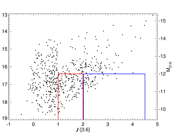
Figure 6: Color-magnitude diagram of [3.6] vs. $J-$[3.6] for targets in the Spitzer and near IR combined catalog. Regions of specific classes of stars as seen in Figure 3 of Bonanos et al. (2009, 2010) are outlined by a red box for RSGs, and a blue box for sgB[e] stars.

In order to expand the massive evolved candidate star list, we used the FourStar data in $J$-band along with the Spitzer 3.6 $\mu$m measurements to construct a plot of [3.6] versus $J-$[3.6] similar to Figure 3 in Bonanos et al. (2009). Figure 6 shows our version of the plot. We have regions of interest outlined in red for the location of spectroscopically known red supergiants in the LMC (Bonanos et al. 2009), 1.0 $<$ $J-$[3.6] $<$ 2.0 and fainter than $M_{\rm[3.6]}=-12$, while the blue outline shows the location of known sgB[e] stars, 2.0 $<$ $J-$[3.6] $<$ 4.5 and fainter than $M_{\rm[3.6]}=-12$. A total of 148 candidates were found in these regions. At the risk of removing possible interesting massive star candidates (massive stars outside of this region due to binary interactions or SN kicks), but increasing our chances of selecting individual massive stars, we again chose to exclude any objects lying outside a box of 10′ centered on the nucleus of M83. When combined with those selected from our analysis of Spitzer observations 31 sources were selected using both sets of criteria, leaving 185 massive star candidates.

3.2.3 High Angular Resolution HST/WFC3 Optical Selection Criteria

Cross referencing coordinates of the 185 candidates selected from near- and mid-IR photometric criteria with positions in the WFC3 images, we visually inspected the area surrounding each candidate and classified it based on its appearance. We ranked each candidate based on the probability of confirming their massive nature via spectroscopic follow up of the target. Rank 1 is used for objects that are the most isolated, with few nearby stars of comparable brightness. Those objects with slightly more crowded fields, but maintaining the appearance of a single star are put into rank 2. In rank 3, fields get more crowded, making identification of the individual objects more difficult. Some objects classified as rank 3 show a diffuse nature. For objects in rank 4, crowding was worse than in rank 3 or objects are even more difficult to recover. Rank 5 is reserved for the worst cases of crowding, diffuse nature of the primary candidate, or a complete lack of recovered object at the position.

The WFC3 fields do not cover all of the disk of M83. Because of this only 112 of the 185 massive star candidates may be checked by visual inspection. This resulted in the identification of 55 ($49\%$) candidates with ranks 1 and 2 for best suited for spectroscopic follow-up observations.

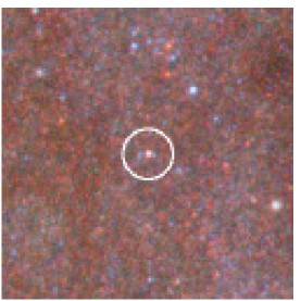
(a)

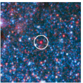
(b)

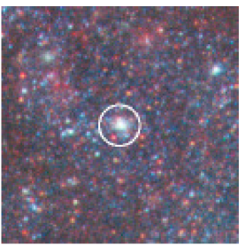
(c)

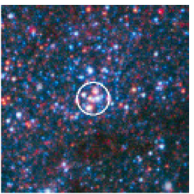
(d)

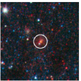
(e)

Figure 7: Composite HST images (from F336W $U$, F438W $B$, F547M $y$, F555W $V$, F657N H$\alpha$, F814W $I$) of objects from Table 3 demonstrating the “Quality” ranks listed in column 15. Both the F336W and F438W filter images make up the blue colors, F547M or F555W images are shown as green, while red colors are from F657N H$\alpha$ and F814W. Each image is 10″ on a side. Over-plotted is the 1$\aas@@fstack{\prime\prime}$7 Spitzer point spread function. The quality ranks are: (a) an isolated, excellent red candidate, rank 1, (b) an extremely red candidate, rank 2, (c) an unresolved cluster or other non-point source, rank 3, (d) a compact association, rank 4, (e) a likely background galaxy, rank 5. In these images, North is up and East is left.

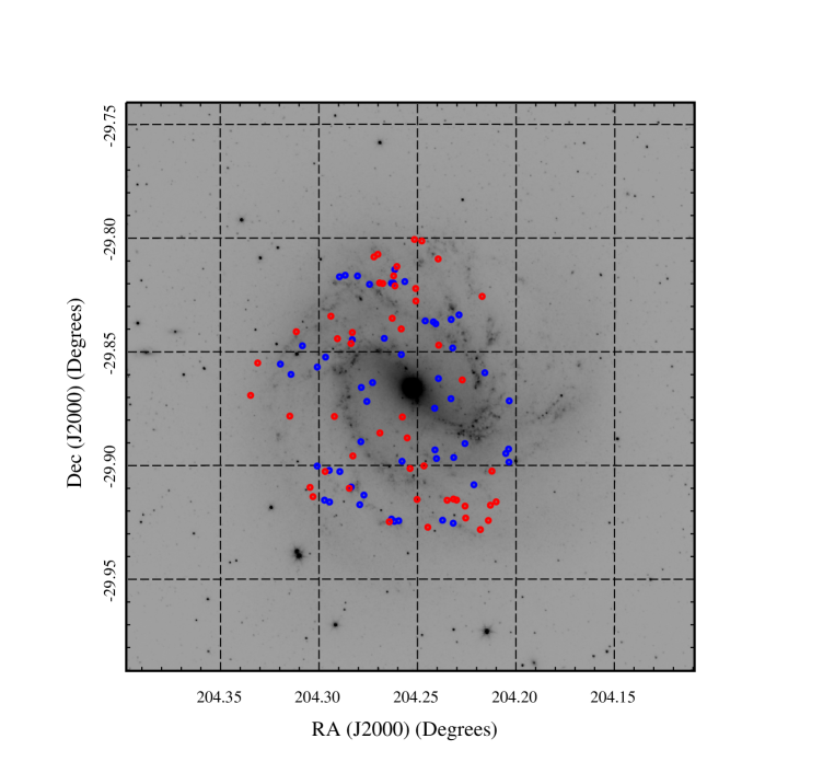
Figure 8: A 15$\arcmin$ $\times$ 15$\arcmin$ Spitzer 3.6 $\mu$m Band 1 image of M83, depicting objects with rank 1 and 2 as red circles, and rank 3 and higher shown as blue circles. All candidates lie within the HST coverage and are in the spiral arms, where massive star candidates are most likely to reside.

Figure 7 shows examples of each rank, 1 through 5, while the online figure set shows a postage stamp for each of the 112 candidates grouped by rank. These ranks, as well as a short comment to explain the rank for each candidate, are given in Table 3 for all 185 candidates selected from IR data. Objects not in the HST field of view have a comment stating as much. Also listed are broadband photometric measurements and uncertainties in Johnson $U,B,V$ and $I$ as well as the available near- and mid-IR photometric measurements. The uncertainties of the HST optical measurements are merely the output from DAOPHOT and have not been more closely checked. They are listed here to give the reader a general idea of the accuracy of the HST photometry. The magnitudes listed in Table 3 are not corrected for either Galactic extinction, nor reddening internal to M83. However, for reference, Galactic extinction is $A_{U}=0.288$, $A_{B}=0.241$, $A_{V}=0.182$, $A_{I}=0.1$ mag from the Schlafly & Finkbeiner (2011) IR-based dust map, and the average M83 internal extinctions from Kim et al. (2012) based on HST observations of the central region are $A_{U}=0.696$, $A_{B}=0.559$, $A_{V}=0.441$, $A_{I}=0.256$ mag. To illustrate the locations of these candidate RSGs, Figure 8 shows the greyscale IRAC Band 1 3.6 $\mu$m image used in the analysis with the sky positions of the candidates overplotted. Candidates of the best rank (ranks 1 and 2) are plotted as red circles, while those of lower quality (ranks 3 through 5) are represented by blue circles.

4 Discussion

There have been several surveys for massive stars that have used broadband optical photometry (e.g. Massey 1998; Levesque & Massey 2012; Grammer & Humphreys 2013) as a principal means to find red, blue, and yellow supergiants. Thus, a comparison of optical versus IR selection techniques is worthy of a brief discussion.

The primary reason to utilize mid-IR observations to explore the massive stellar content of a galaxy is that evolved massive stars, with substantial dust or circumstellar material, will be more easily detectable in the IR as opposed to the optical. Deep optical photometry of galaxies has not been conducted in a systematic fashion beyond the Local Group Galaxy Survey effort of Massey et al. (2006). Plus, mid-IR selection criteria have been shown successful in the Local Group after spectroscopic follow up (Britavskiy et al. 2014).

One drawback with the current mid-IR surveys is the difference in resolution compared to near-IR and optical images. Massive stars are born, and mostly die, in clusters or associations, meaning spatial resolution at the distance of M83 is a prominent concern. The PSF of the near-IR observations is just below 1^′′ corresponding to a size of 23 pc at M83’s distance. This size is smaller than the 40 pc size of the Spitzer PSF, but may still easily include clusters, associations or several stars. OB associations can have half-light radii of a few parsecs and extend over several tens of parsecs, while young massive clusters can exist in a volume less than one cubic parsec (Clark et al. 2005). One such example is the cluster Stephenson 2, which contains roughly 30 RSGs in a radius between 3.2 and 4.2 pc (Negueruela et al. 2012). The regions of M83 covered by the seven HST fields have an order of magnitude better resolution than the FourStar observations. This PSF corresponds to $\sim$0$\aas@@fstack{\prime\prime}$1 or just over 2 pc. While some objects may still be compact clusters, we can eliminate many objects that are larger than 2 pc in size, increasing our odds of observing only individual stars with follow-up spectroscopy.

The second issue with using mid-IR data concerns the limiting magnitude attainable. We found absolute magnitude limits of M${}_{[3.6]}\simeq-10.1$ mag for the completeness of the survey, meaning we are completely sensitive to only the brightest RSGs at the distance of M83. Similarly, Khan et al. (2010) noted that for NGC 6946 at a distance of 5.6 Mpc, the 3$\sigma$ detection limit in the 4.5 $\mu$m band corresponded to an absolute magnitude of close to $-10$. Therefore, given the limits in both photometry and resolution, mid-IR studies intended to study the stellar content of galaxies beyond $\sim$5 Mpc with current archival data from Spitzer will be severely limited.

Ideal candidates are those that are isolated and meet photometric criteria in the IR that have been previously successfully used to identify massive stars. Because we have deep optical photometry (from the HST images) for our IR selected candidates, we can explore the differences and similarities in selecting candidates using IR photometry versus selecting candidates using optical photometry.

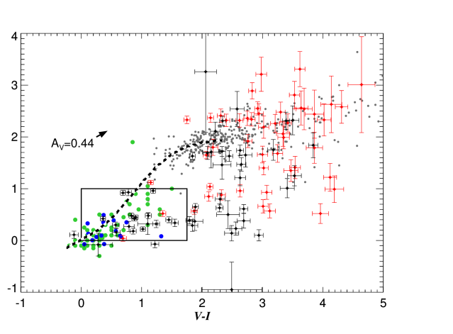
Figure 9: Color-color diagram for M83 stars with HST photometry. Objects determined to be good candidates for follow-up spectroscopy with rank 1 and 2 are shown in red, while objects with ranks 3 and higher are shown in black. Also plotted is a “typical” $V$-band reddening for stars in M83’s central region as reported by Kim et al. (2012). Spectroscopically confirmed RSGs in the Local Group are collectively shown as grey points. The dashed line represents the theoretical supergiant sequence from Bertelli et al. (1994) as used in Grammer & Humphreys (2013). The box outlines the region where cluster candidates are known to exist (Barmby et al. 2006). The blue points are sgB[e] stars from the LMC and SMC (Bonanos et al. 2009, 2010), while the green points are blue supergiants from M31 and M33 (Humphreys et al. 2014).

In pioneering the effort to find red supergiants in nearby galaxies, Massey (1998) showed that while both the $V-R$ and $B-V$ photometric colors change with effective temperature, $B-V$ also changes with surface gravity, and can therefore be used to uniquely identify RSGs from foreground, Milky Way red halo stars. A similar approach was implemented by Grammer & Humphreys (2013) with $B-V$ and $V-I$ colors. Grammer & Humphreys (2013) extracted a theoretical supergiant sequence from the stellar models of Bertelli et al. (1994) to further illustrate the usefulness of such a color-color diagram in selecting massive star candidates. Ten of the 112 candidates visually inspected in the HST images were not recovered in one or more of the filters needed for plotting on this color-color diagram. Figure 9 shows the 102 (of 112) candidates listed in Table 3 with $B$, $V$, and $I$ magnitudes on a color-color diagram of $B-V$ versus $V-I$. In total, there are 49 candidates with rank 2 or lower plotted in red in Figure 9 and 53 candidates with a rank higher than 2 plotted in black. Of the 49 highly ranked visually inspected candidates, 24 (49%) lie in the region of the color-color diagram similar to the RSG candidates of Grammer & Humphreys (2013). Within uncertainties, another four strong candidates also lie within this region. Based on the location of our candidates on the similar plot of $B-V$ versus $V-I$, we expect that $\sim$50% of the strong (49 red points in Figure 9) candidates we selected via near- and mid-IR photometry are truly RSGs. To be certain, we need follow-up spectroscopy to confirm this hypothesis. For comparison, Massey (1998) applied a photometric cutoff in the $B-V$ versus $V-R$ colors, then performed spectroscopic follow-up observations in order to confirm the objects as RSGs and found that for the faintest candidates, the success rate of the optical photometric criteria in selecting RSGs was 82%. To compare our expected success rate of recovering RSGs with that from optical surveys, we must note a few caveats. First, the optical photometry used by Massey et al. (2009), for example, is much more accurate than the photometry from the HST data. This is simply due to the much greater distance to the stars in M83 than to the studied stars in Local Group galaxies. The second caveat relates also to the accuracy of the photometry, this time from Spitzer. Selection criteria are only as good as the accuracy of the photometry, and as can be seen in Figures 2 and 3, within uncertainties, some RSG candidates may move in and out of the region encompassed by our selection criteria. Because of these caveats, our predicted RSG success rate is lower than that from optical observations.

To aid in illustrating where confirmed RSGs reside, in Figure 9 we have plotted spectroscopically confirmed RSGs (grey dots) from the Local Group that have $B$, $V$, and $I$-band measurements: 119 from M31 that are not labeled as “crowded” objects (Massey et al. 2009), 46 from M33 that are not “multiple” (Massey et al. 2006), 73 from the Milky Way (Ducati 2002; Levesque et al. 2005, and references therein), 41 from the LMC (Bonanos et al. 2009), 19 from the SMC (Bonanos et al. 2010), and 30 from the Dwarf Irregular galaxies (dIrrs) in the Local Group (Levesque & Massey 2012; Britavskiy et al. 2014; Britavskiy et al. in prep.). The box outlines the region described in Grammer & Humphreys (2013) where Barmby et al. (2006) show that cluster candidates exist. Interestingly, this region also is predominantly the locus of the massive stars such as sgB[e] from Bonanos et al. (2009, 2010) (blue dots), and the list of LBVs, LBV candidates, Fe ii emission line stars, and other (blue) supergiants in M31 and M33 from Humphreys et al. (2014) shown as green dots. Comparing our candidates with the locations of the spectroscopically classified massive stars from the literature, objects in the upper right of the plot are most likely RSGs, while those in the lower left are their bluer massive star counterparts. The average reddening (Kim et al. 2012) is shown as an arrow, meaning some candidates outside the described regions are simply reddened RSGs in the upper part of the plot, or reddened sgB[e] stars (for example) in the lower central part of the plot. The strong candidates (red dots) in the lower right part of the plot are not very red in $B-V$ while being quite red in $V-I$. Grammer & Humphreys (2013) put forth the explanation that objects in the bottom right of the color-color diagram may contain blended objects or compact H ii regions. Indeed, at the limit of the HST resolution, ultra compact H ii regions, which are typically connected to small clusters of stars (Conti et al. 2008), may be contaminants. In a study of the clusters in the central fields of the HST data for M83, Chandar et al. (2010) show that reddening may cause the $V-I$ values of candidate LBVs to move out of where they are expected in the same way as seen in our plot. Whitmore & the WFC3 Science Oversight Committee (2011) and Kim et al. (2012) bring up the possibility that these objects may be the chance superposition of a red and a blue star. Spectroscopic follow-up is the only way to definitively determine the nature of these objects as either reddened LBVs, a superposition of two different kinds of stars or simply clusters of stars. It should also be mentioned that Massey et al. (2009) discussed that 5 of 19 spectroscopically confirmed RSGs in M31 from Massey (1998) would not have met their photometric criteria. They stressed that RSGs may exist in other regions of the color-color diagram, but reiterated the point that their optically photometric criteria have a superb success rate of $>82$% (Massey 1998) at selecting RSGs based on confirmation from follow-up spectroscopy. Again, this is higher than our expected $\sim$50% success rate based on IR photometry.

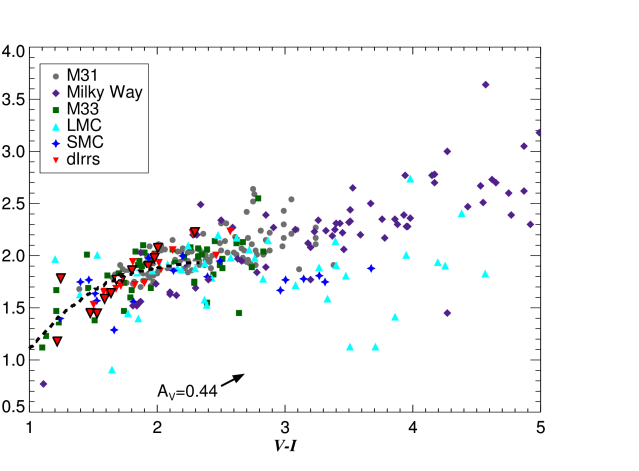
Figure 10: A color-color diagram showing the locations of spectroscopically confirmed RSGs broken down by galaxy in the Local Group. Over-plotted is the theoretical supergiant sequence from Grammer & Humphreys (2013) and Bertelli et al. (1994), as well as an arrow showing the typical reddening in M83 as determined by Kim et al. (2012).

How does selecting evolved massive stars via IR photometry compare with the Massey (1998) optical selection method? Plotted in Figure 10 by color and galaxy are the spectroscopically confirmed RSGs shown in grey in Figure 9. Also plotted is the supergiant sequence from Grammer & Humphreys (2013) and Bertelli et al. (1994) for reference. Because optical surveys were performed first and are thus more numerous and typically have better resolution, a very small number of confirmed RSGs come from the IR-selected candidates in dIrrs (Britavskiy et al. 2014; Britavskiy et al. in prep.), which are shown as red triangles outlined in black. The spectroscopically confirmed IR-selected candidates in the dIrrs in the Local Group lie in exactly the same region as those spectroscopically confirmed RSGs selected via optical photometry, and are represented by downward pointing red triangles that are not outlined in black. Clearly, there are too few RSGs selected via the IR to draw strong conclusions, but these first few attest to the usefulness of selecting RSGs from IR observations. Looking further at the plot, there are a few interesting possibilities that will be confirmed or rejected with more observations. For the confirmed RSGs in the SMC in Figure 10, are the six RSGs with lower $B-V$ representative of a metallicity effect? These RSGs are all K-type, and the trend of earlier average spectral type of RSGs with decreasing metallicity of the host galaxy has been shown by Levesque & Massey (2012). More observations of RSGs in metal-poor galaxies are needed to confirm or refute this possible trend. The Local Group dIrr RSGs do not yet have deep enough photometry to indicate if this trend is real. Another question raised by this plot is why do the LMC RSGs, Milky Way RSGs, and M83 RSGs suffer from so much scatter on this plot?

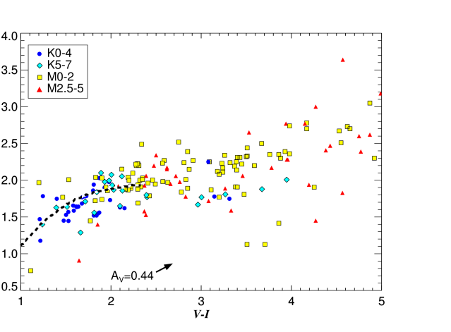
Figure 11: A color-color diagram showing the locations of spectroscopically confirmed RSGs in the Local Group broken down by spectral type. Over-plotted is the theoretical supergiant sequence from Grammer & Humphreys (2013) and Bertelli et al. (1994).

In Figure 11 we plot RSGs grouped by four spectral types: early K, late K, early M, and late M. The K spectral type RSGs appear less reddened, and show less scatter. This follows from the intrinsic bluer colors of K-type RSGs compared to M-types. However, K-type RSGs also appear to have less reddening than their later-type companions. This is likely due to the fact they come from, on average, lower metallicity galaxies. One interesting possibility for this scatter for the later-type RSGs may be related to the behavior of HV 11423 in the SMC. Massey et al. (2007) tracked HV 11423 through changes in its spectral type from K0 I to M5 I. The star changed by 2 mag in $V$, with changes in spectral type attributed to both the change in effective temperature, and the creation and dissipation of dust (Massey et al. 2007). HV 11423 is an exceptional case, but it would be interesting to investigate via long term observations whether the scatter of later spectral types in Figure 11 is connected with a cycle of production and destruction of dust.

What kind of RSGs do we expect to find in M83? The average spectral type for RSGs in the Milky Way is M2 (Levesque & Massey 2012). The disk metallicity of M83 was shown to be 1.9$\times$ Solar by Gazak et al. (2014). Thus, we may expect the average spectral type of an M83 disk RSG to be M2 or later. In addition, we may expect the typical M83 RSG to experience greater mass loss rates, as mass loss rates tend to increase with later spectral type.

5 Conclusions

We present point source catalogs for a 15$\arcmin$ $\times$ 15$\arcmin$ region centered on M83 based on Spitzer mid-IR and near-IR photometry. From these catalogs, we have selected candidate massive stars based on their mid- and near-IR photometric properties. These candidates have been culled by checking against catalogs of known objects, and also by inspection on high resolution HST images. The remaining 49 objects are strong candidates for evolved massive stars, and await follow-up spectroscopy to further determine their nature and quantify the success rate of this technique in detecting evolved massive stars.

We make the full catalog of point sources available to the community in order, for example, for future researchers to characterize the progenitors of core-collapse SNe. The methodology used in this paper may be readily applied to other nearby ($\leq 5$ Mpc) galaxies to investigate their evolved massive stellar populations. High quality archival Spitzer images exist for all nearby ($\leq 10$ Mpc) galaxies courtesy of the SINGS and LVL surveys (Kennicutt et al. 2003; Dale et al. 2009). Archival HST images also exist for many of the nearby galaxies. Analysis of follow-up spectroscopy of candidates discussed here for M83 will be needed to further test this methodology. However, studies starting merely with Spitzer photometry have already proved to be successful in discovering evolved massive stars (Britavskiy et al. 2014; Britavskiy et al. in prep.). The validation of the usefulness of this IR method of determining massive star candidates is important, especially because in many cases, deep optical photometry simply does not exist. This method may also provide an alternative to the previously employed optical methods to investigate the massive stellar content of the Local Universe.

Table 1: Infrared Photometry of 4528 Point Sources in the field of M83

RA(J2000)	Dec(J2000)	$J$	$\sigma_{J}$	$K_{\rm s}$	$\sigma_{K_{\rm s}}$	[3.6]	$\sigma_{3.6}$	[4.5]	$\sigma_{4.5}$	[5.8]	$\sigma_{5.8}$	…
(deg)	(deg)	(mag)	(mag)	(mag)	(mag)	(mag)	(mag)	(mag)	(mag)	(mag)	(mag)	…
204.16129	–29.85840	16.40	0.02	16.01	0.03	15.91	0.03	16.03	0.07	14.90	0.07	…
204.16831	–29.90027	17.42	0.03	16.52	0.03	17.02	0.04	17.27	0.11	17.09	0.28	…
204.17050	–29.81191	16.64	0.02	16.27	0.05	16.47	0.05	16.60	0.06	16.21	0.11	…
204.17440	–29.86086	18.31	0.05	16.65	0.06	16.73	0.06	16.99	0.08	13.31	0.01	…
204.18935	–29.91848	16.28	0.01	15.86	0.02	15.91	0.04	16.07	0.05	15.01	0.04	…
204.20567	–29.92462	17.81	0.04	16.80	0.05	16.77	0.05	17.01	0.07	16.31	0.25	…
204.21006	–29.91604	18.40	0.05	16.71	0.05	16.85	0.05	17.08	0.07	13.79	0.03	…
204.21704	–29.83906	17.41	0.03	16.40	0.04	16.70	0.05	16.84	0.05	13.46	0.17	…
204.22253	–29.82444	17.43	0.05	15.97	0.06	15.55	0.04	15.66	0.06	15.92	0.76	…
204.23417	–29.94974	19.66	0.15	16.94	0.10	16.37	0.03	16.50	0.06	15.82	0.11	…

This table is available in its entirety in a machine-readable form in the online journal. A portion is shown here for guidance regarding its form and content.

Table 2: FourStar Photometry Compared to 2MASS Photometry

2MASS ID	$J_{\rm PSF}$	$J_{\rm 2MASS}$	Difference	$(J-K_{\rm{s}})_{\rm FourStar}$	$(J-K_{\rm{s}})_{\rm 2MASS}$	Difference
	(mag)	(mag)	(mag)	(mag)	(mag)	(mag)
13372193–2947529	15.761(10)	15.694(58)	0.067	0.889(23)	0.888(141)	0.001
13371693–2947174	16.105(8)	16.067(88)	0.038	0.896(21)	0.850(188)	0.046
13371216–2948184	16.235(15)	16.192(99)	0.043	1.027(37)	0.923(195)	0.104
13364314–2947289	15.781(12)	15.872(77)	–0.091	0.981(46)	0.947(145)	0.034
13364385–2949437	15.427(11)	15.448(63)	–0.020	0.767(42)	0.634(130)	0.133
13363909–2949390	15.696(7)	15.729(77)	–0.033	0.284(28)	0.242(226)	0.042
13363400–2949388	16.011(12)	16.000(82)	0.011	0.708(41)	0.852(164)	–0.144
13363098–2950437	15.155(10)	15.194(48)	–0.039	0.850(36)	0.806(91)	0.044
13363542–2953303	16.219(10)	16.366(130)	–0.147	0.993(24)	0.950(250)	0.043
13370045–2957177	15.670(7)	15.712(65)	–0.042	0.487(25)	0.463(178)	0.024
13370527–2956231	15.962(10)	15.939(80)	0.023	1.076(26)	1.057(146)	0.019
13372091–2949532	15.234(9)	15.249(47)	–0.015	0.844(19)	0.884(89)	–0.040

Table 3: Massive Evolved Star Candidates in M83 from $HST$, Near-IR, and $Spitzer$ Photometry

RA(J2000)	Dec(J2000)	$U$	$\sigma_{U}$	$B$	$\sigma_{B}$	$V$	$\sigma_{V}$	$I$	$\sigma_{I}$	$J$	…
(deg)	(deg)	(mag)	(mag)	(mag)	(mag)	(mag)	(mag)	(mag)	(mag)	(mag)	…
204.27068	–29.78285	. . .	. . .	. . .	. . .	. . .	. . .	. . .	. . .	18.07	…
204.27253	–29.78501	. . .	. . .	. . .	. . .	. . .	. . .	. . .	. . .	. . .	…
204.17782	–29.78529	. . .	. . .	. . .	. . .	. . .	. . .	. . .	. . .	. . .	…
204.33232	–29.78565	. . .	. . .	. . .	. . .	. . .	. . .	. . .	. . .	. . .	…
204.25152	–29.80064	26.67	0.37	26.56	0.18	24.08	0.07	20.78	0.03	18.74	…
204.24779	–29.80129	26.90	0.42	25.79	0.13	23.43	0.05	20.68	0.03	18.46	…
204.27008	–29.80718	25.25	0.19	24.72	0.08	22.35	0.04	20.21	0.03	18.28	…
204.31808	–29.80785	. . .	. . .	. . .	. . .	. . .	. . .	. . .	. . .	. . .	…
204.27208	–29.80829	. . .	. . .	29.69	0.90	26.68	0.22	22.04	0.04	18.94	…
204.23951	–29.80921	26.16	0.30	27.44	0.27	25.65	0.13	21.79	0.04	18.66	…

This table is available in its entirety in a machine-readable form in the online journal. A portion is shown here for guidance regarding its form and content.

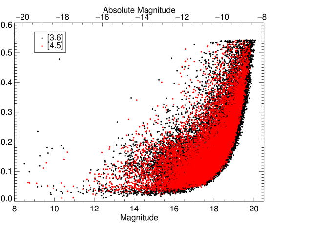
Figure 1: Magnitude versus uncertainty for the Spitzer [3.6] and [4.5] point sources. The [4.5] values are in red and show both the higher uncertainties and brighter limiting magnitude limit for this bandpass.

Figure 4: Comparison of the $J$ magnitude from FourStar PSF measurements to the $J$ magnitude from 2MASS. Note the much smaller uncertainties for data from FourStar as compared to data from 2MASS.

Figure 5: Comparison of the $(J-K_{\rm s})$ from FourStar PSF measurements to the $(J-K_{\rm s})$ from 2MASS. Again, FourStar measurements have much smaller uncertainties.

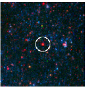
(a)

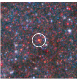
(b)

(c)

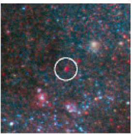
(d)

(e)

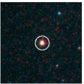
(f)

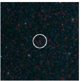
(g)

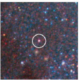
(h)

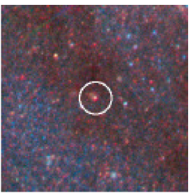
(i)

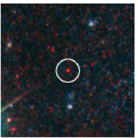
(j)

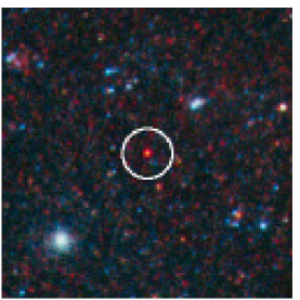
(k)

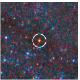
(l)

Figure 12: Objects from Table 3 with a rank of 1, thus excellent candidates for a massive star. The color scheme for these images is the same as for Figure 7. Each image is 10″ on a side, with the Spitzer point spread function of 1$\aas@@fstack{\prime\prime}$7 shown as a white circle. North is up and East is left.

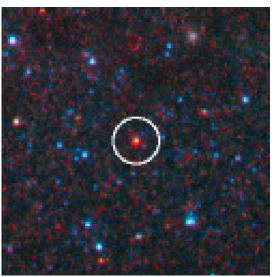
(a)

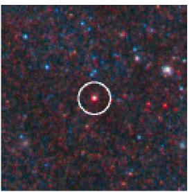
(b)

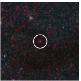
(c)

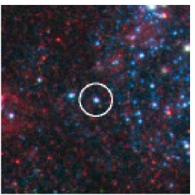
(d)

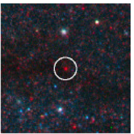
(e)

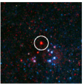
(f)

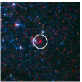
(g)

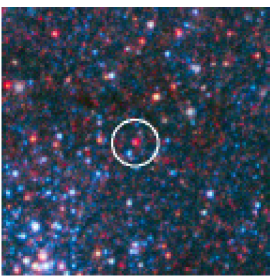
(h)

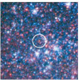
(i)

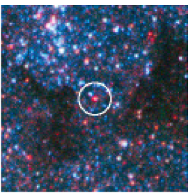
(j)

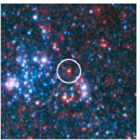
(k)

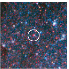
(l)

Figure 13: More objects from Table 3 with a rank of 1, thus excellent candidates for a massive star. The color scheme for these images is the same as for Figure 7. Each image is 10″ on a side, with the Spitzer point spread function of 1$\aas@@fstack{\prime\prime}$7 shown as a white circle. North is up and East is left.

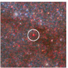
(a)

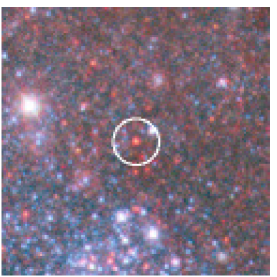
(b)

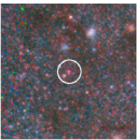
(c)

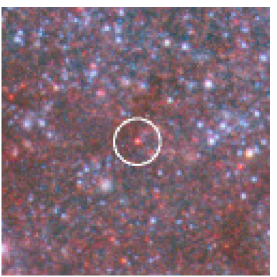
(d)

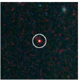
(e)

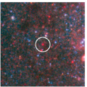
(f)

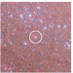
(g)

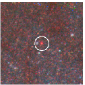
(h)

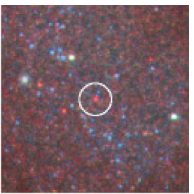
(i)

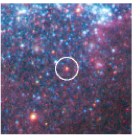
(j)

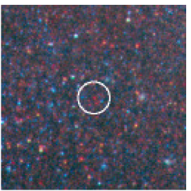
(k)

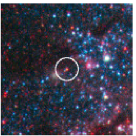
(l)

Figure 14: More objects from Table 3 with a rank of 1, thus excellent candidates for a massive star. The color scheme for these images is the same as for Figure 7. Each image is 10″ on a side, with the Spitzer point spread function of 1$\aas@@fstack{\prime\prime}$7 shown as a white circle. North is up and East is left.

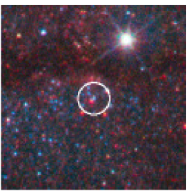
(a)

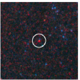
(b)

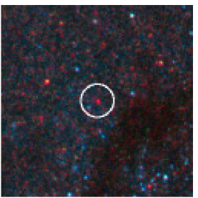
(c)

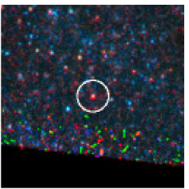
(d)

Figure 15: More objects from Table 3 with a rank of 1, thus excellent candidates for a massive star. The color scheme for these images is the same as for Figure 7. Each image is 10″ on a side, with the Spitzer point spread function of 1$\aas@@fstack{\prime\prime}$7 shown as a white circle. North is up and East is left.

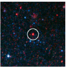
(a)

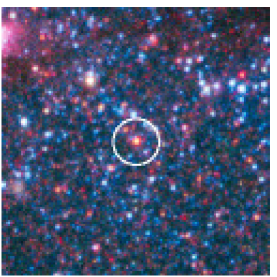
(b)

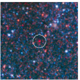
(c)

(d)

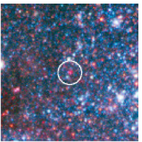
(e)

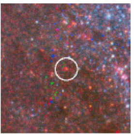
(f)

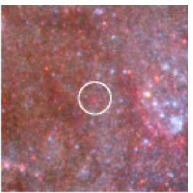
(g)

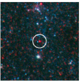
(h)

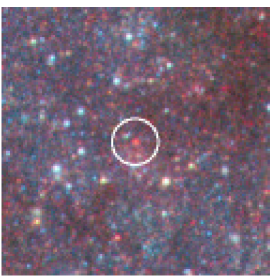
(i)

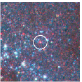
(j)

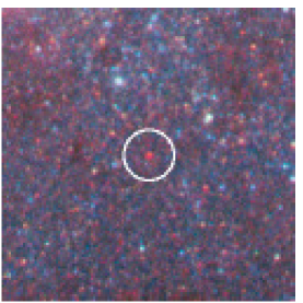
(k)

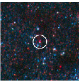
(l)

Figure 16: Objects from Table 3 with a rank of 2, thus decent candidates for a massive star. The color scheme for these images is the same as for Figure 7. Each image is 10″ on a side, with the Spitzer point spread function of 1$\aas@@fstack{\prime\prime}$7 shown as a white circle. North is up and East is left.

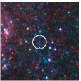
(a)

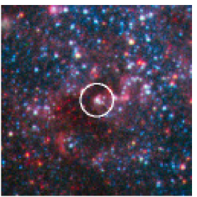
(b)

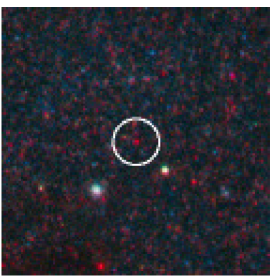
(c)

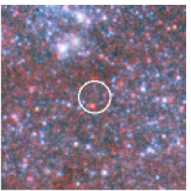
(d)

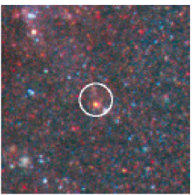
(e)

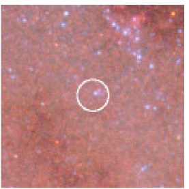
(f)

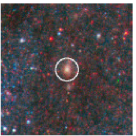
(g)

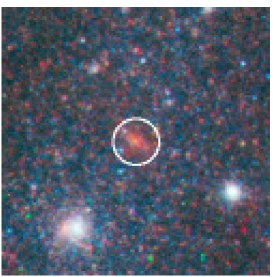
(h)

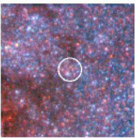
(i)

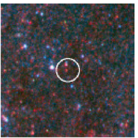
(j)

Figure 17: More objects from Table 3 with a rank of 2, thus decent candidates for a massive star. The color scheme for these images is the same as for Figure 7. Each image is 10″ on a side, with the Spitzer point spread function of 1$\aas@@fstack{\prime\prime}$7 shown as a white circle. North is up and East is left.

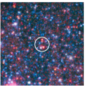
(a)

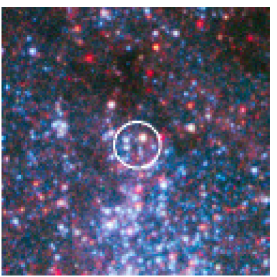
(b)

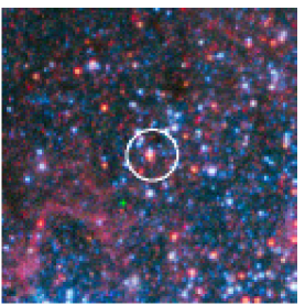
(c)

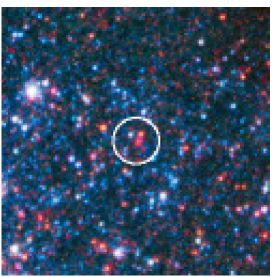
(d)

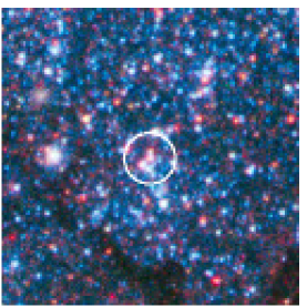
(e)

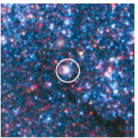
(f)

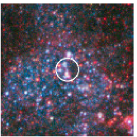
(g)

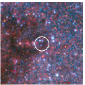
(h)

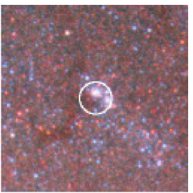
(i)

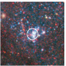
(j)

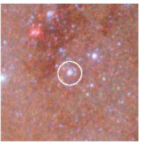
(k)

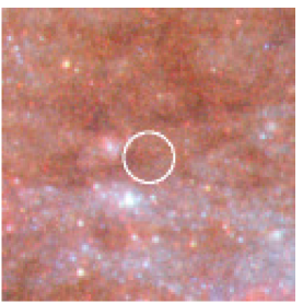
(l)

Figure 18: Objects from Table 3 with a rank of 3, thus not good candidates for a massive star. The color scheme for these images is the same as for Figure 7. Each image is 10″ on a side, with the Spitzer point spread function of 1$\aas@@fstack{\prime\prime}$7 shown as a white circle. North is up and East is left.

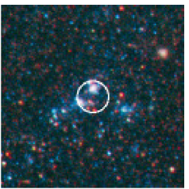
(a)

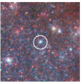
(b)

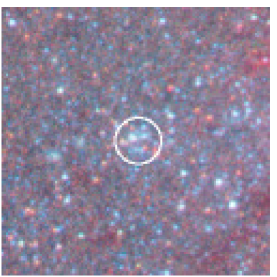
(c)

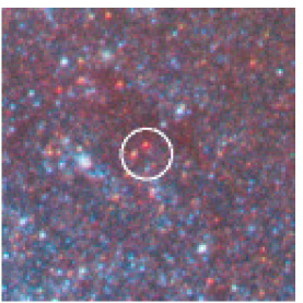
(d)

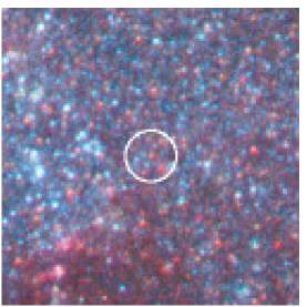
(e)

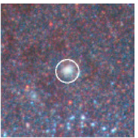
(f)

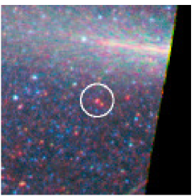
(g)

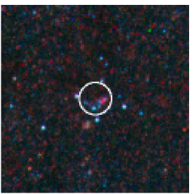
(h)

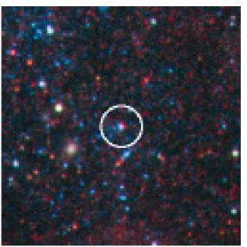
(i)

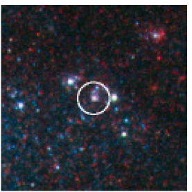
(j)

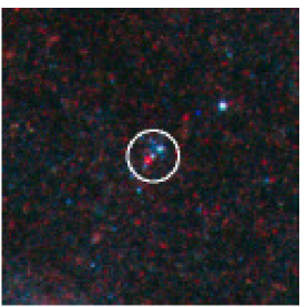
(k)

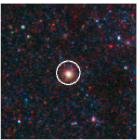
(l)

Figure 19: More objects from Table 3 with a rank of 3, thus not good candidates for a massive star. The color scheme for these images is the same as for Figure 7. Each image is 10″ on a side, with the Spitzer point spread function of 1$\aas@@fstack{\prime\prime}$7 shown as a white circle. North is up and East is left.

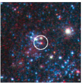
(a)

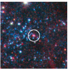
(b)

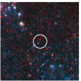
(c)

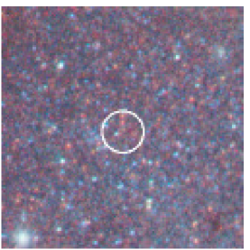
(d)

Figure 20: More objects from Table 3 with a rank of 3, thus not good candidates for a massive star. The color scheme for these images is the same as for Figure 7. Each image is 10″ on a side, with the Spitzer point spread function of 1$\aas@@fstack{\prime\prime}$7 shown as a white circle. North is up and East is left.

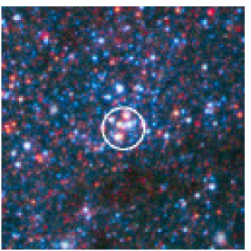
(a)

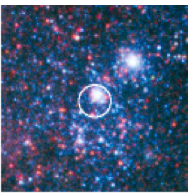
(b)

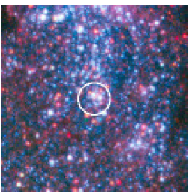
(c)

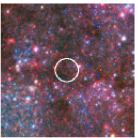
(d)

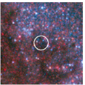
(e)

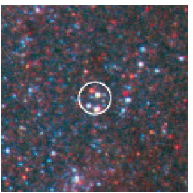
(f)

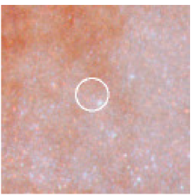
(g)

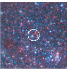
(h)

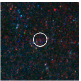
(i)

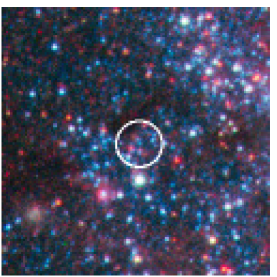
(j)

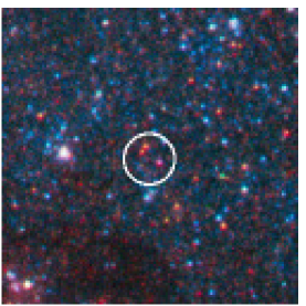
(k)

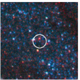
(l)

Figure 21: Objects from Table 3 with a rank of 4, thus very poor candidates for a massive star. The color scheme for these images is the same as for Figure 7. Each image is 10″ on a side, with the Spitzer point spread function of 1$\aas@@fstack{\prime\prime}$7 shown as a white circle. North is up and East is left.

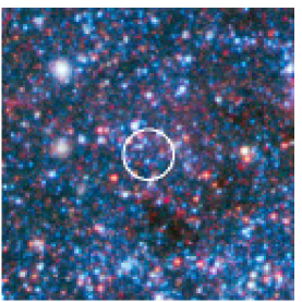
(a)

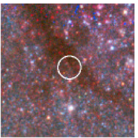
(b)

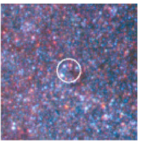
(c)

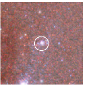
(d)

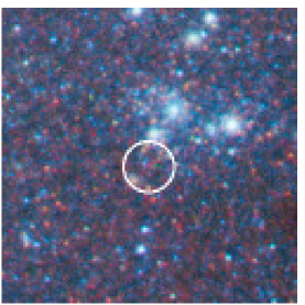
(e)

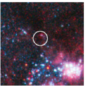
(f)

Figure 22: More objects from Table 3 with a rank of 4, thus very poor candidates for a massive star. The color scheme for these images is the same as for Figure 7. Each image is 10″ on a side, with the Spitzer point spread function of 1$\aas@@fstack{\prime\prime}$7 shown as a white circle. North is up and East is left.

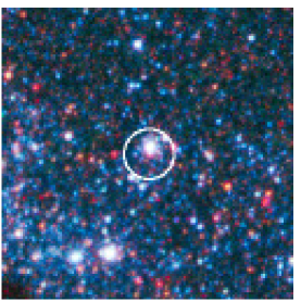
(a)

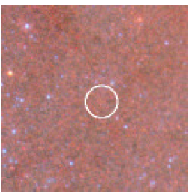
(b)

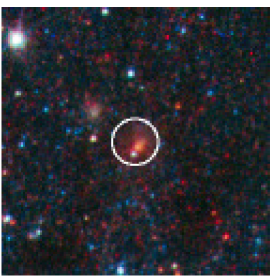
(c)

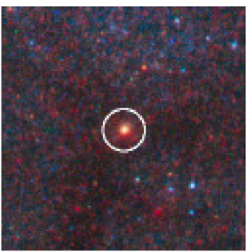
(d)

Figure 23: Objects from Table 3 with a rank of 5, thus extremely poor candidates for a massive star. The color scheme for these images is the same as for Figure 7. Each image is 10″ on a side, with the Spitzer point spread function of 1$\aas@@fstack{\prime\prime}$7 shown as a white circle. North is up and East is left.