Bootstrapping dielectronic recombination from second-row elements and the Orion Nebula

Abstract

Dielectronic recombination (DR) is the dominant recombination process for most heavy elements in photoionized clouds. Accurate DR rates for a species can be predicted when the positions of autoionizing states are known. Unfortunately such data are not available for most third and higher-row elements. This introduces an uncertainty that is especially acute for photoionized clouds, where the low temperatures mean that DR occurs energetically through very low-lying autoionizing states. This paper discusses S${}^{2+}\rightarrow$ S⁺ DR, the process that is largely responsible for establishing the [S III]/[S II] ratio in nebulae. We derive an empirical rate coefficient using a novel method for second-row ions, which do have accurate data. Photoionization models are used to reproduce the [O III] / [O II] / [O I] / [Ne III] intensity ratios in central regions of the Orion Nebula. O and Ne have accurate atomic data and can be used to derive an empirical S${}^{2+}\rightarrow$ S⁺ DR rate coefficient at $\sim 10^{4}$ K. We present new calculations of the DR rate coefficient for S${}^{2+}\rightarrow$ S⁺ and quantify how uncertainties in the autoionizing level positions affect it. The empirical and theoretical results are combined and we derive a simple fit to the resulting rate coefficient at all temperatures for incorporation into spectral synthesis codes. This method can be used to derive empirical DR rates for other ions, provided that good observations of several stages of ionization of O and Ne are available.

1 Introduction

Although numerical simulations are the best way to understand the message in astronomical spectroscopic observations, they can be no better than the underlying atomic and molecular data. Theoretical predictions of cross sections and rate coefficients provide the vast majority of the data now used. There are, however, still significant gaps in the database. Given the amount of effort that has been expended in the past it is inevitable that today’s outstanding needs are also the most challenging ones. Dielectronic recombination (DR), the subject of this paper, is usually the dominant recombination process for heavy elements in photoionized nebulae. The graduate text Osterbrock & Ferland (2006) gives an overall introduction to the physics of photoionized clouds, while Ferland & Savin (2001), Ferland (2003), Savin et al. (2012), and Badnell et al. (2003) review the data needs and the DR process. Nikolić et al. (2013) show how zero-density total DR rate coefficients can be modified to take account of its suppression at finite densities. Ferland (2003) identifies DR and charge exchange as the two most uncertain processes affecting the spectroscopy of photoionized clouds. Here we consider the rates for S${}^{2+}\rightarrow$S⁺ radiative and dielectronic recombination.

Low-temperature DR occurs through low-lying autoionizing resonances (Nussbaumer & Storey, 1983) and is particularly sensitive to their position via the exponent of the Maxwellian distribution. However, it is inherently difficult to calculate their energy position relative to threshold accurately enough and, indeed, whether they reside above or below threshold in the first place. As a result of this “threshold straddling” effect, ab initio theory cannot predict the near threshold DR resonance strength precisely enough and, ideally, theoretical efforts should be guided by experimentally observed positions of autoionizing states in order to produce accurate DR rate coefficients at all temperatures (Schippers et al., 2004). This is especially important for photoionized clouds because the gas kinetic temperature is low and so the rate is strongly affected by the position of any such low-lying resonances. Such experimental energies are not available for S⁺ so uncertainties in the positions of the resonances are a source of error, although estimates have been made (Badnell, 1991; Nahar, 1995). Although these uncertainties are widely understood, we know of no calculations which demonstrate them in detail. We present such calculations in Section 3 below.

Simulations of nebulae can be used to infer the existence of overlooked processes, and estimate rates for dominant reactions. For example, Pequignot et al. (1978) inferred the existence of fast charge-exchange reactions between atomic hydrogen and doubly ionized oxygen from models of a planetary nebula. In the next section we use the Baldwin et al. (1991) model of the Orion Nebula, together with today’s advanced stellar atmosphere spectral energy distributions (SEDs) and atomic data, to derive an improved photoionization model. We reproduce the observed [O I], [O II], [O III], and [Ne III] spectra, produced by ions for which accurate atomic data is available, and derive an empirical S${}^{2+}\rightarrow$S⁺ DR rate coefficient at $T\sim 10^{4}$ K. Section 3 presents new calculations of the S${}^{2+}\rightarrow$ S⁺ radiative and dielectronic recombination rate coefficients, examines the sensitivity of the DR rate coefficient to the detailed atomic structure, obtains a theoretical rate coefficient which agrees with the empirical rate coefficient at $10^{4}$ K, and investigates its uncertainty over a broader temperature range. This bootstrap approach can be used to derive DR rate coefficients for other species using observations of [O I], [O II], [O III], and [Ne III].

2 Bootstrapping S DR from second-row elements in the Orion H II region

Baldwin et al. (1991) (hereafter BFM) used Cloudy to construct a photoionization model of the Orion Nebula. They reproduced the observed intensities of roughly two dozen emission lines that form in the H⁺ layer, including lines of [O II] $\lambda$3727, [O III] $\lambda\lambda$4363, 5007, [S II] $\lambda$6725 and [S III] $\lambda$9532 We improve upon this model here.

2.1 Improved atomic and grain physics

We use the most recent stellar SEDs and atomic data, as described below. The BFM model, and differences between today’s assumptions and those used in 1991, are described here. We use version 13.03 of Cloudy, last described by Ferland et al. (2013). This has a nearly complete revision of the atomic database in the 20+ years since BFM was completed. Some details are given in Ferland et al. (1998) and Ferland et al. (2013). Nearly all aspects of the database have changed, but improvements in the physics of dielectronic recombination have been substantial, as outlined below.

BFM included a self-consistent treatment of grains, including gas heating by photoejection of electrons, grain heating by both the stellar continuum and internally generated radiation, and collisions between grains and the surrounding plasma. The grain emission was predicted and found to be in good agreement with observations, showing that most of the warm dust emission originates in the H⁺ region. Our grain treatment has been updated, as described in van Hoof et al. (2004) and Ferland et al. (2013). As discussed in the first reference, these changes predict less photoelectric heating than was found with the older theory used by BFM. In our current calculation each grain population is resolved into ten sized bins. Two grain types, an astronomical silicate and graphitic material, are included. The size distribution is altered as described by BFM to reproduce the relatively grey opacities observed in Orion.

2.2 Geometry

The BFM model was of a hydrostatic plane-parallel layer on the surface of the background molecular cloud. The ionized gas was assumed to be in hydrostatic equilibrium (termed “constant pressure” in that paper, since all forces balanced) with the outward momentum of the absorbed stellar continuum being balanced by the sum of gas and line radiation pressure. We also assume hydrostatic equilibrium here. A detailed model of the geometry of the H II region was derived by Wen & O’Dell (1995).

BFM worked in terms of the flux of ionizing photons striking the plane-parallel layer, using Cloudy in its so-called “intensity case”, in which only the flux of photons is specified. The distance of the stars can be derived from this flux and an assumed calibration of the O-star luminosity function. We adopt the stellar parameters and SED described below, which are significantly different from those assumed in BFM, and reflect advances in our understanding of O stars. For these parameters, the physical separation between the Trapezium stars and the illuminated face of the H⁺ layer ($3.15\times 10^{17}$ cm) is not large compared with the thickness of the layer ($6\times 10^{16}$ cm) so the stellar radiation field will suffer some spherical dilution as it passes across the layer. This is taken into account by using Cloudy’s “luminosity case”, in which the stellar luminosity and star-cloud separation are specified. This affects the intensities of low-ionization lines.

2.3 Stellar SED

The use of modern stellar SEDs is the largest source of differences between the calculations presented here and those of BFM. The SED of the central star cluster is fundamental because it is the source of heating and ionization in the H⁺ layer. BFM used the Kurucz (1979) plane parallel LTE SEDs, the most extensive grids of stellar atmosphere calculations available at that time. These are now known to produce too soft a radiation field (Sellmaier et al., 1996). Several modern stellar atmosphere grids, including TLUSTY (Lanz & Hubeny, 2003) and WMBasic (Pauldrach et al., 2001), are now available. These are thought to give a better representation of the SED at ionizing energies (Simón-Díaz & Stasińska, 2008). The spectral classes given by Simón-Díaz et al. (2006) are used.

Figure 1 compares the Atlas (used by BFM), WMBasic, and TLUSTY SEDs for the same stellar temperature and luminosity. The major differences are at photon energies $h\nu\geq 35$ eV, with the modern calculations $\sim 1$ dex brighter than Atlas. This solves a puzzle found by BFM. They required a high Ne abundance to reproduce the optical [Ne III] lines. [Ne III] is the highest ionization species seen in the spectrum of an H II region. For reference, Figure 1 also shows the ionization potentials of the ions discussed in this paper. O stars have little radiation with h$\nu>54$ eV. The high Ne abundance derived by BFM compensated for the deficiency of photons at energies capable of producing Ne²⁺ in the Atlas SED. A cosmic Ne abundance is obtained when the modern SED is used, as discussed below.

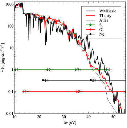
Figure 1: Stellar SED and ions of interest. The Atlas SED was used by BFM while this work employs WMBasic predictions. The SED predicted by TLUSTY is also shown. The horizontal lines indicate ionization potentials for the O, Ne, and S ions discussed in this paper.

We adopted the WMBasic grid of SEDs. These include NLTE and the effects of mass loss and winds (Pauldrach et al., 1998). All are important in OB stars. Simón-Díaz & Stasińska (2008) compare various SEDs and find that WMBasic reproduces the ionization of H II regions, and that it is preferred above 35 eV for supergiants with effective temperatures $\sim 40$ kK, which have parameters similar to the stars in Orion.

2.4 Final model parameters

Wagle et al (in preparation) describe the updated Orion Nebula model in detail. Most aspects of the improved model are similar to BFM. Table 1 summarizes model parameters. The first entry gives the temperature of $\theta^{1}$ Ori C, the brightest star in the Trapezium cluster. The flux of hydrogen-ionizing photons striking the nebula is denoted by $\phi$(H). The abundances for the interstellar medium (ISM) described in Jenkins (2009) were used as a reference. The abundances are similar, as expected for a newly formed H II region. Table 2 gives some predictions, derived using the DR rate coefficients determined below. Most lines are well fitted by the model. The Table also illustrates some problems with astronomical observations. The model fits the [O III] $\lambda 5007$Å  and [O II] $\lambda 7325$Å lines quite well, and fits [O II] $\lambda 3727$Å within 2$\sigma$. The UV line is especially uncertain because it lies on the extreme short wavelength edge of the spectrum observed by BFM.

Table 1: Model parameters for the Orion Nebula.

Parameter value $T_{*}(\theta^{1}{\rm OriC})$ 38,950 K Radius 3.15$\times 10^{17}$ cm $\phi$(H) 5.9$\times 10^{12}$ cm^-2 O/H 3.66$\times 10^{-4}$ Ne/H 1.29$\times 10^{-4}$ S/H 1.36$\times 10^{-4}$

Table 2: Model predictions for the Orion Nebula.

Line Observed Predicted / Observed S(H$\beta$)  erg  cm^-2 s^-1 arcsec^-2 4.63$\times 10^{-12}$ $\pm$0.4 1.02 $[$O II$]$ 3727/H$\beta$ 0.94$\pm$0.2 0.64 $[$Ne III$]$ 3869/H$\beta$ 0.2$\pm$0.03 0.85 $[$O III$]$ 5007/H$\beta$ 3.43$\pm$0.17 1.06 $[$S II$]$ 6720/H$\beta$ 0.051$\pm$0.003 1.01 $[$O II$]$ 7325/H$\beta$ 0.1191$\pm$0.006 0.88 $[$S III$]$ 9530/H$\beta$ 1.445$\pm$0.285 1.00

2.5 The [Ne III]/[O III]/[O II]/[O I] bootstrap

Figure 1 suggests that oxygen / neon spectra can be used to infer rates for S${}^{2+}\rightarrow$S⁺ recombination. Second-row elements have relatively complete spectroscopic data, accurate recombination rate coefficients, and are readily available (e.g. http://amdpp.phys.strath.ac.uk/tamoc/DR/). The observed oxygen ions are produced by the stellar SED between 13.5 eV and 54 eV, while [Ne III] is produced by photons between 40 eV and 54 eV. The relative distribution of these four ions depends on the shape of the stellar SED (Figure 1) and on the intensity of ionizing radiation striking the layer, as described in the text Osterbrock & Ferland (2006).

The problem is overdetermined — we have two variables and three ionization ratios, counting only second-row ions with good atomic data. This would guarantee that the [S III] / [S II] ratio is properly reproduced since, as shown by Figure 1, the S ions lie within the range covered by the O and Ne ions. In effect, the S ionization interpolates on the observed and reproduced O & Ne ionization. The S DR rate is poorly constrained, but the O and Ne ions, with their good recombination rates, can be used to bootstrap one.

Figure 2 illustrates this idea. The right panel shows the ratio of [Ne III] to [O III]. Ne²⁺ has the highest ionization potential of any ion in an H II region, so this ratio is mainly sensitive to the stellar temperature, with little dependence on stellar luminosity. The ratio then, in effect, sets the stellar temperature.

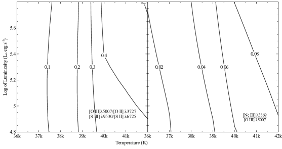
Figure 2: Predicted O, S, and Ne spectra are shown as a function of the two free parameters in the model, the stellar temperature, which sets the SED shape, and the stellar luminosity, which sets the intensity of starlight falling upon the H⁺ layer. The [Ne III]/[O III] ratio shown in the right panel sets the stellar temperature, which then sets the [O III]/[O II] / [S III]/[S II] shown in the left panel. The S²⁺ recombination rate is the only additional parameter affecting the left panel.

The left panel shows the ratio of ratios, [O III]/[O II] / [S III]/[S II]. The ratio of ratios depends mainly on stellar temperature because the O²⁺ – O⁺ and S²⁺ – S⁺ ionization potentials do not match exactly, so, the fractional abundance ratios change asynchronously. The stellar temperature is set to good precision by the [Ne III]/[O III]. The only degree of freedom that can change the left panel is the total S${}^{2+}\rightarrow$S⁺ recombination rate.

The total S${}^{2+}\rightarrow$S⁺ recombination rate is the sum of a well-determined radiative recombination (RR) rate, an uncertain dielectronic recombination rate, and possibly charge exchange (CX) recombination. Kingdon & Ferland (1996) find that S${}^{2+}\rightarrow$S⁺ CX does not have an open channel so most likely occurs by very slow radiative CX, with a rate coefficient $\sim 10^{-17}$ cm³ s^-1. We adopt the RR rate coefficient given below, which is in good agreement with that found by Aldrovandi & Pequignot (1973). We adjusted the DR rate coefficient to reproduce the observed ratio of ratios to make Figure 2. The resulting best-fit DR rate coefficient is $3\times 10^{-12}$ cm³ s${}^{-1}\pm 0.2$ dex at $10^{4}$ K, which we refer to as our empirical value. This kinetic temperature is measured using ratios of [O III] forbidden lines, as outlined in Chapter 5 of Osterbrock & Ferland (2006). In this way the well-understood atomic physics of O and Ne can be used to bootstrap a rate for species lacking the required spectroscopic data.

We experimented with other SEDs during the course of this work. We initially used the TLUSTY grid, which is somewhat harder than Atlas but softer than WMBasic (Figure 1). We were able to reproduce the oxygen spectrum using TLUSTY, and simultaneously, the S${}^{2+}-$S⁺ balance, with a DR rate of $6\times 10^{-12}$ cm³ s^-1. However, a neon abundance significantly above the cosmic value was needed to offset the softness of the SED, the same problem that forced a high neon abundance in BFM. We prefer to take the neon abundance as a prior, which then drives the selection of the SED and the DR rate.

We adopt the solar Ne/H ratio recommended by Asplund et al. (2009). This is based on spectroscopic observations of nearby B stars and should reflect the composition of the local ISM. Ne is an inert gas and so should not form chemical compounds which then form grains, so its depletion should be low. The gas-phase neon abundance of the Orion H II region should be close to the values obtained from early-type stars.

Having obtained a best fit DR rate coefficient we can then vary it to quantify how the line spectrum depends on it. Strong forbidden lines arising from low-lying levels are predominantly formed by impact excitation with thermal electrons. Because of this, changes in the DR rate change the spectrum mainly through changes in the fraction of S that is doubly ionized. This is shown in Figure 3. The main effect of increasing the DR rate coefficient is to increase the intensity of the [S II] lines. S²⁺ is the dominant stage of ionization in the H⁺ region, with only $\sim 3$% of S being singly ionized (BFM). Increasing the DR rate increases the fraction of S⁺ significantly while having a more modest effect on the S²⁺ fraction. The O lines are hardly affected by changes in the S DR rate. There are small changes in [O II] intensities caused by changes in the gas kinetic temperature as a result of the changing intensities of the [S II] lines.

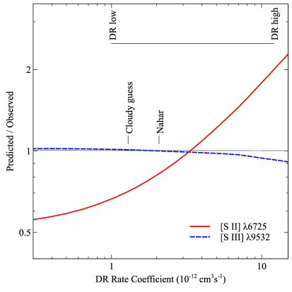
Figure 3: The ratio of predicted to observed line intensities of S lines are shown as a function of the S${}^{2+}\rightarrow$S⁺ DR rate coefficient. A DR rate coefficient of $3\times 10^{-12}$ cm³ s${}^{-1}\pm 0.2$ dex is indicated.

Figure 3 also shows other estimates of the DR rate coefficient. Nahar (1995) gives the sum of the RR and DR rate coefficients. We subtracted the Aldrovandi & Pequignot (1973) RR rate coefficient to obtain a Nahar “DR rate coefficient” of 2.1$\times 10^{-12}$ cm³ s^-1 at 10⁴ K. Cloudy uses mean DR rate coefficients for those species not covered by modern calculations, as described by Ali et al. (1991). The mean for S²⁺ is 1.5$\times 10^{-12}$ cm³ s^-1 at $10^{4}$ K. Thus, our empirical total DR+RR rate coefficient is 50% larger at $10^{4}$ K. The atomic calculations described below find values within the range indicated at the top of the figure.

3 Dielectronic Recombination Calculations for S²⁺ Producing S⁺

The previous section has derived a S${}^{2+}\rightarrow$S⁺ benchmark DR rate coefficient of $3\times 10^{-12}$ cm³ s${}^{-1}\pm 0.2$ dex at $10^{4}$ K. Here we describe the atomic physics aspects of the DR calculations, and quantify the present uncertainties at low temperature associated with low-lying, near-threshold resonances. The previously-derived rate coefficient is found to be within the rather large range of possible computed values. We use that derived benchmark to constrain our atomic model, and then compute a consistent DR rate coefficient for all temperatures.

The relevant DR and RR processes are as follows. An electron incident on the $3s^{2}3p^{2}(^{3}P_{0})$ ground state of S²⁺ can either directly recombine (i.e., via RR) into any final bound state $3s^{2}3p^{2}(^{3}P_{0})nl$ ($3\leq n\leq\infty$) or it may first be captured into a particular resonance state that subsequently decays radiatively to a final bound state (DR):

$$e^{-}+3s^{2}3p^{2}(^{3}P_{j}) \longrightarrow \left\{\begin{array}[]{ll}3s^{2}3p3dnl&3p\rightarrow 3d\ {\rm dipole\ resonances}\\ 3s3p^{3}nl&3s\rightarrow 3p\ {\rm dipole\ resonances}\\ 3s^{2}3p^{2}(^{3}P_{j^{\prime}})nl&{\rm fine-structure\ resonances}\\ 3s^{i}3p^{j}3d^{5-i-j}&(N+1)-{\rm electron\ resonances}\end{array}\right.$$ (8)

$$(RR)\searrow \ \ \ \ \ \ \downarrow\ (DR)$$

$$\left\{\begin{array}[]{l}3s^{2}3p^{3}\\ 3s^{2}3p^{2}nl\\ \end{array}\right\}+h\nu\ .$$

We treat DR and RR independently and proceed to describe the wavefunctions of the initial S²⁺ target states, the intermediate resonance states S${}^{+\,**}$, and the final recombined states $3s^{2}3l_{1}3l_{2}nl$, where we consider all $n_{i}=3$ shell orbitals $3l_{i}=\{3s,3p,3d\}$. We perform all calculations using the atomic structure and collision code AUTOSTRUCTURE (Badnell, 2011), as applied to numerous DR (Badnell et al., 2003) and RR (Badnell, 2006a) calculations.

As a means of perspective, we first show the available DR and RR rate coefficient data that was available prior to the present study in Figure 4.

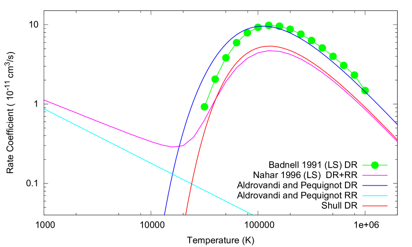
Figure 4: Comparison of previously existing S²⁺ DR and RR rate coefficients: the LS DR AUTOSTRUCTURE results of Badnell (1991) (green); the LS DR-plus-RR R-matrix results of Nahar (1995) (magenta); the DR (blue) and RR (cyan) results of Aldrovandi & Pequignot (1973); the DR results of Shull (red).

A prominent high-temperature peak is present in all the DR results, due to the dipole core-excited contributions in Eq. 8, but there are minimal features seen at lower temperatures — essentially the RR contribution only here. (It is helpful to note that the R-matrix results of Nahar (1995) include by necessity the coherent contributions of DR and RR.)

Our theoretical treatment for improvement on the existing DR data begins by including relativistic effects to first-order via the Breit-Pauli Hamiltonian (the previous LS calculations of Badnell (1991) and Nahar (1995) shown in Fig. 4 were non-relativistic) and follows similar recent work on DR of the isoelectronic Fe¹²⁺ (Badnell, 2006b) and the isonuclear S³⁺ (Abdel-Naby et al., 2012) ions. As in Badnell (2006b), the atomic basis used to describe the S²⁺ target states consists of Thomas-Fermi orbitals $\{1s,2s,2p,3s,3p,3d\}$ with the same scaling argument $\lambda=1.13$ for all orbitals, which was chosen so as to reproduce the fine-structure splitting of the $3s^{2}3p^{2}(^{3}P_{j})$ levels as compared to NIST (see Table 3).

Table 3: Energies (Ryd) of the S²⁺ target states.

Level	Present	NIST
$3s^{2}3p^{2}\,(^{3}P_{0})$	0.000000	0.000000
$3s^{2}3p^{2}\,(^{3}P_{1})$	0.002712	0.002722
$3s^{2}3p^{2}\,(^{3}P_{2})$	0.007638	0.007591
$3s^{2}3p^{2}\,(^{1}D_{2})$	0.128824	0.103180
$3s^{2}3p^{2}\,(^{1}S_{0})$	0.268614	0.247509
$3s3p^{3}\,(^{5}S_{2})$	0.469658	0.534658
$3s3p^{3}\,(^{3}D_{1})$	0.747518	0.765640
$3s3p^{3}\,(^{3}D_{2})$	0.747707	0.765890
$3s3p^{3}\,(^{3}D_{3})$	0.748146	0.766370
$3s3p^{3}\,(^{3}P_{2})$	0.888483	0.899833
$3s3p^{3}\,(^{3}P_{1})$	0.888986	0.900021
$3s3p^{3}\,(^{3}P_{0})$	0.889175	0.900078
$3s^{2}3p3d\,(^{1}D_{2})$	0.944683	0.949173
$3s^{2}3p3d\,(^{3}F_{2})$	1.101637	1.112826
$3s^{2}3p3d\,(^{3}F_{3})$	1.104230	1.115427
$3s^{2}3p3d\,(^{3}F_{4})$	1.107787	1.119023
$3s3p^{3}\,(^{1}P_{1})$	1.298494	1.247012
$3s3p^{3}\,(^{3}S_{1})$	1.307283	1.258155
$3s^{2}3p3d\,(^{3}P_{0})$	1.323255	1.303996
$3s^{2}3p3d\,(^{3}P_{1})$	1.325432	1.304182
$3s^{2}3p3d\,(^{3}P_{2})$	1.326393	1.304254
$3s^{2}3p3d\,(^{3}D_{1})$	1.357430	1.344589
$3s^{2}3p3d\,(^{3}D_{2})$	1.358329	1.345870
$3s^{2}3p3d\,(^{3}D_{3})$	1.359080	1.346358
$3s3p^{3}\,(^{1}D_{2})$	1.440140	1.384930
$3s^{2}3p3d\,(^{1}F_{3})$	1.460029	1.436251
$3s^{2}3p3d\,(^{1}P_{1})$	1.551177	1.495763

Within this orbital basis, we include intra-shell correlation configurations, most importantly, those arising from $3s^{2}\rightarrow 3p^{2}$ two-electron promotion, giving a target state configuration basis of $\{3s^{2}3p^{2},3s3p^{3},3s^{2}3p3d,3s3p^{2}3d,3s^{2}3d^{2},3s3p3d^{2},3s3d^{3},3p^{3}3d,3p^{2}3d^{2},3p3d^{3}\}$. By then performing a large-scale configuration-interaction calculation, including relativistic corrections to lowest order, we obtain the S²⁺ target energies listed in Table 3. While the present computed energies tend to align fairly well with the recommended NIST values, especially for the fine-structure-split states, we note theoretical energy overestimates of up to 0.05 Ryd for the higher-lying states. The dominant high-temperature DR rate coefficient is due to the core dipole transitions in Eq. 8, which are governed by the strongest core radiative rates, and so we list those in Table 4. The computed rates agree to within $\approx 10\%$ of the NIST values.

Table 4: The three strongest radiative rates $A_{r}$ ($\times 10^{9}$ s^-1) from dipole-core-excited states of S²⁺ to the $3s^{2}3p^{2}\,(^{3}P_{0})$ ground state.

Transition			Present	NIST
$3s3p^{3}\,(^{3}S_{1})$	$\rightarrow$	$3s^{2}3p^{2}\,(^{3}P_{0})$	1.82	1.60
$3s^{2}3p3d\,(^{3}P_{1})$	$\rightarrow$	$3s^{2}3p^{2}\,(^{3}P_{0})$	3.51	3.87
$3s^{2}3p3d\,(^{3}D_{1})$	$\rightarrow$	$3s^{2}3p^{2}\,(^{3}P_{0})$	7.27	6.93

Having adequately represented the N-electron target states of S²⁺, we then describe the various states of S⁺ taking part in Eq. 8 by a basis consisting of either a distorted-wave continuum ($\epsilon l$) or a valence orbital ($nl$) coupled to each of the S²⁺ target configurations, plus the so-called $(N+1)$-electron target-orbital basis: $3s^{2}3p^{3}$, $3s^{2}3p^{2}3d$, $3s^{2}3p3d^{2}$, $3s3p^{4}$, $3s3p^{3}3d$, $3s3p^{2}3d^{2}$, $3s^{2}3d^{3}$, $3s3p3d^{3}$, $3p^{5}$, $3p^{4}3d$, and $3p^{3}3d^{2}$ (all $N+1=15$ electrons occupy a target orbital $nl=\{1s,2s,2p,3s,3p,3d\}$). Many of these latter $(N+1)$-electron configurations have strong capture and radiative rates, and also give rise to near-threshold bound or resonance states, so they may play an important part in the low-temperature DR process, as will be seen. Within this large basis set, DR cross sections and Maxwellian-averaged rate coefficients are then computed, and these initial results are depicted in Figure 5. The upper panel shows the three strong ground core dipole-excited $3s3p^{3}(^{3}S_{1})nl$ and $3s^{2}3p3d(^{3}P_{1}\,\,\&\,\,^{3}D_{1})nl$ resonance series converging to their respective thresholds ($\approx 1.25-1.35$ Ryd, as indicated in Table 3). The second panel from the top focuses on the low-lying $(N+1)$-electron resonances, in particular the strong $3s3p^{3}3d(^{4}D_{7/2})$ state at 0.321 Ryd (see, also, Table 5). The third panel highlights the $3s^{2}3p^{2}(^{3}P_{1,2})nl$ spin-orbit-split series; these dominate the near-threshold energy region (as long as there are no strong low-lying $(N+1)$-electron resonances). In the bottom panel, the resultant Maxwellian-averaged rate coefficient indicates that there is a large high-temperature peak due to the core dipole-excited series, and then a mild rise at low temperature due to the spin-orbit-split series near threshold.

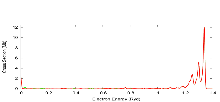
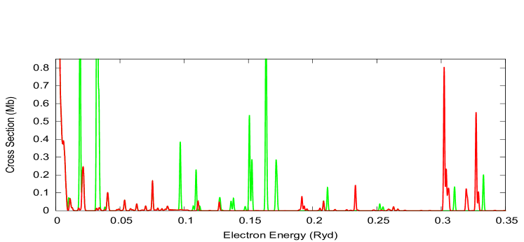
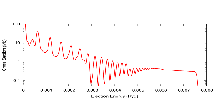
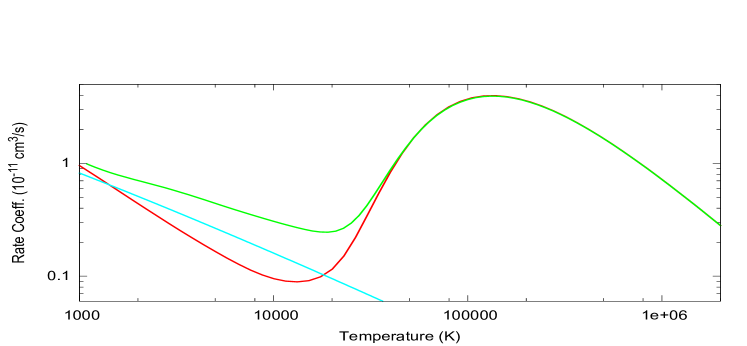
Figure 5: S²⁺ DR cross section (upper three panels, convolved with FWHM Gaussians convolutions of 0.01, 0.001, and 0.0001 Ryd in descending order) and Maxwellian-averaged rate coefficient (lower panel). Ab initio results are in red and those with all $(N+1)$-electron resonances shifted by -0.157 Ryd are in green. The computed RR rate coefficient is the cyan curve in the lower panel.

It is apparent from Figure 5 that at the temperature of interest — $10^{4}$ K, corresponding to an electron energy of about 0.06 Ryd — the DR rate coefficient is determined by the sum of three contributions: 1) the lower-temperature tail of the large contribution from dipole-excited resonances, 2) the higher-temperature tail of the near-threshold spin-orbit-split resonances, and 3) the $n=3$ $(N+1)$-electron resonances, with uncertain resonance positions. We note that while contributions 1) and 2) are subject to suppression at finite densities, according to Nikolić et al. (2013), contribution 3) is not.

Upon closer scrutiny of the energies of the $(N+1)$-electron bound states and resonances, and by comparing to available NIST bound state data, it is found that our limited (for computational feasibility) atomic description results in a general overestimate of these latter energies. In Table 5, we list three prominent $(N+1)$-electron S⁺ bound state energies — for the $3s3p^{4}\,(^{2}S_{1/2})$, $3s3p^{4}\,(^{2}P_{3/2})$, and $3s3p^{4}\,(^{2}P_{1/2})$ states. Relative to the S${}^{2+}3s^{2}3p^{2}\,(^{3}P_{0})$ threshold, corresponding to zero incident electron energy in the DR process, the theoretically-predicted energies are overestimated by $\approx 0.25-0.45$ Ryd. Also listed in this table is the strong S${}^{+}\,3s3p^{3}3d\,(^{4}D_{7/2})$ resonance, which has a theoretically-predicted energy position of $\approx 0.32$ Ryd (there are no available NIST or other data for this autoionizing energy position, to our knowledge). Given the overestimate of the corresponding bound $(N+1)$-electron energies, it is reasonable to infer that the energy of this autoionizing resonance is likewise overestimated, and that the “true” resonance position should be closer to threshold; this suggests that the “true” DR rate coefficient at $T=10^{4}$ K could be enhanced by the presence of such a strong resonance, compared to a computed rate coefficient where the theoretical resonance position is at higher energy. More generally, we expect the entire manifold of $(N+1)$-electron resonances to be positioned too high and so there may be similar contributions (DR enhancements) from a group of suitably re-positioned resonances.

To understand how the DR rate coefficient at $T=10^{4}$ depends on the precise position of a strong resonance, consider that, for an isolated resonance, the rate coefficient is given by

$$\alpha^{{\rm DR}}_{i}(T) \approx constant\times T^{-3/2}{\rm e}^{-E_{i}/kT}\ ,$$

where $E_{i}$ is the resonance position. For a given resonance strength, this contribution at $T=10^{4}\ (kT\approx 0.06\,{\rm Ryd})$ increases as the resonance position approaches threshold. For example, the enhancement to the $T=10^{4}$ rate coefficient by repositioning, or shifting, a single resonance from $E_{i}=0.32$ Ryd to $E_{i}^{shift}\approx 0$ is given by the factor ${\rm e}^{+E_{i}/kT}\approx{\rm e}^{0.32/0.06}\approx 200$. This example illustrates how uncertainties in resonance positions can translate into rather large uncertainties in the low-temperature DR rate coefficient. (At higher temperatures, any energy uncertainty is small compared to $kT$ so that there is far less sensitivity to the exact resonance position.)

Table 5: Energies (Ryd) of the S⁺ ground state and selected $(N+1)$-electron bound and resonance states, compared to the S²⁺ ground state. The present theoretical energies for $3s$-vacancy states, which are subject to relaxation effects, relative to the ground state of S²⁺, are overestimated by $\approx 0.2-0.4$ Ryd., as highlighted in boldfaced font.

		$E-E_{3s^{2}3p^{3}\,(^{4}S_{3/2})}$		$E-E_{3s^{2}3p^{2}\,(^{3}P_{0})}$
Ionic State		Present	NIST	Present	NIST	Overestimate
S+	$3s^{2}3p^{3}\,(^{4}S_{3/2})$	0.000	0.000	-1.630	-1.715
S+	$3s3p^{4}\,(^{2}S_{1/2})$	1.455	1.092	-0.175	-0.623	+0.448
S+	$3s3p^{4}\,(^{2}P_{3/2})$	1.488	1.326	-0.142	-0.389	+0.247
S+	$3s3p^{4}\,(^{2}P_{1/2})$	1.493	1.329	-0.137	-0.386	+0.249
S2+	$3s^{2}3p^{2}\,(^{3}P_{0})$	1.630	1.715	0.000	0.000
S+	$3s3p^{3}3d\,(^{4}D_{7/2})$	1.951		0.321

Guided by our initial supposition that the computed low-lying resonance energy positions are overestimated, we wish to investigate the effect of resonance position uncertainties on the low-temperature DR rate coefficient by performing two new DR calculations in which the $(N+1)$-electron resonance positions are shifted. In the first case, a global $(N+1)$-electron resonance shift of -0.32 Ryd was applied in order to realign the strongest S${}^{+}\,3s3p^{3}3d\,(^{4}D_{7/2})$ resonance to just above threshold (at +0.001 Ryd), thereby maximizing the resulting low-temperature rate coefficient. In the second case, a global shift of -0.157 Ryd was used, positioning instead that resonance at only 0.163 Ryd above threshold, but yielding a total DR rate coefficient of $3\times 10^{-12}$ cm³/s at $T=10^{4}$ K, consistent with the value derived in the previous section.

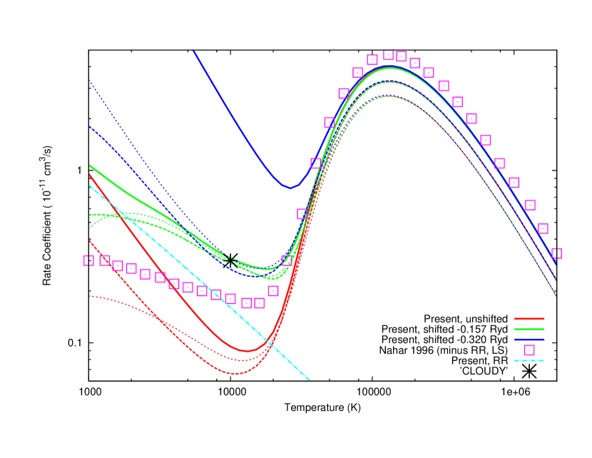
Figure 6: A comparison of S²⁺ DR and RR rate coefficients, including the breakdown of DR from the $3s^{2}3p^{2}(^{3}P_{j})$ ground ($j=0$, solid) and metastable ($j=1$, long-dashed) and ($j=2$, short-dashed) levels. The red curve indicates the ab initio calculations, where the strong $3s3p^{3}3d(^{4}D_{7/2})$ resonance is positioned at 0.321 Ryd above threshold. The blue curve corresponds to an empirical shift of all $n=3$ $(N+1)$-electron resonances by -0.32 Ryd so as to reposition the $3s3p^{3}3d(^{4}D_{7/2})$ resonances just above the $j=0$ ground state threshold, giving a maximum $j=0$ low-temperature rate coefficient. The green curve represents an artificial shift somewhere in between (-0.157 Ryd) which yields a statistically-averaged rate coefficient at $T=10^{4}$ K (see Table 6) consistent with the Cloudy deduced value (black asterisk) of $3\times 10^{-12}$ cm³/s. Also shown are the present RR results (cyan curve) and an estimate of the DR contribution from Nahar (1995) (magenta curve).

The computed DR rate coefficients are shown in Figure 6 for all three cases — ab initio (no shift), a shift of -0.32 Ryd, and a shift of -0.157 Ryd — and each case is further resolved by the various initial $3s^{2}3p^{2}(^{3}P_{j})$ levels, with $j=0$ corresponding to the ground state of S²⁺ and $j=1,2$ being the first two spin-orbit-split excited states (see Table 3). At lower temperatures, in particular, at $T=10^{4}$ K, the rate coefficient varies by about an order of magnitude between the ab initio results and the $-0.32$ Ryd shifted results. It should be noted, however, that the latter case corresponds to the optimal shift scenario in which the strongest resonance was positioned closest to threshold. Furthermore, this fortuitous positioning of the strong resonance just above the $j=0$ ground state (therefore below the two $j=1$ and $j=2$ excited states) results in a larger enhancement in the ground-state rate coefficient compared to the excited-state rate coefficients. In such cases where the various $j$-resolved results differ significantly, an observation-based rate coefficient could be used in conjunction with the theoretically-predicted $j$ variations to obtain density diagnostics.

Table 6: Computed S²⁺ DR and RR recombination rate coefficients (cm³ s^-1) evaluated at $T=10^{4}$ K. The computed results are resolved by ground ($j=0$) and metastable ($j=1$ and $j=2$) $3s^{2}3p^{2}(^{3}P_{j})$ initial states. The computed statistical averages and the high-density limit (HDL) derived rate coefficients are also listed.

$j$ DR RR 0 3.08E-12 1.60E-12 1 2.82E-12 1.59E-12 2 2.98E-12 1.50E-12 Avg. 2.94E-12 1.54E-12 HDL 3.10E-12 1.54E-12

The last case involved an intermediate scenario in which the $(N+1$)-electron resonances were shifted by $-0.157$ Ryd. This particular shift was chosen so as to produce a statistically-averaged (over initial $j$ levels) DR rate coefficient in line with the high-density limit (HDL) value of $3\times 10^{-12}$ cm³/s derived earlier (see Table 6, which lists the various DR and RR rate coefficients at $T=10^{4}$ K). Thus we have bootstrapped our DR calculations, that were initially suspect due to uncertainties in the $(N+1$)-electron resonance positions, by choosing a plausible shift of these resonances in order to reproduce a computed rate coefficient that agrees with the benchmark value at $T=10^{4}$ K.

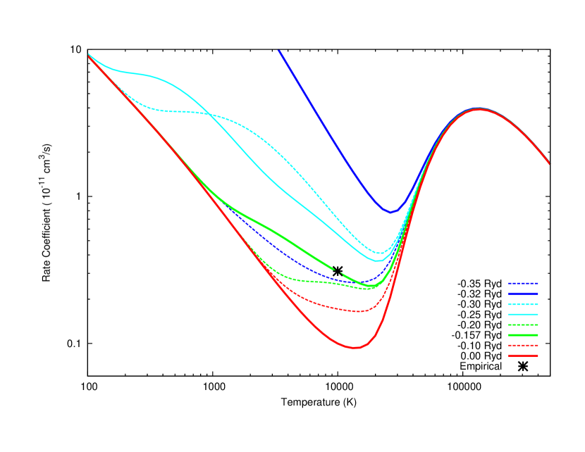
Figure 7: DR rate coefficients for electrons incident on the S${}^{2+}(3s^{2}3p^{2}\,{}^{3}P_{0})$ ground state, subject to a uniform shift in energy position of all $(N+1)$-electron resonances. The shifted energies for each case are shown in the legend, and the present observationally-derived empirical rate coefficient of $3.10\times 10^{-12}$ cm³/s at $T=10^{4}$ K is also shown.

To extend the usefulness of this approach to other photoionized plasmas (e.g. over $10^{3}-10^{4}$ K), we need to examine the spread of any family of curves, corresponding to different shifts, say, but which pass through our point at $10^{4}$ K. We do this in Figure 7, for the ground level only now. Of particular note are the three curves, with shifts of -0.20, and -0.35 Ryd, plus our original -0.157 Ryd. While all three are consistent with our empirical value at $10^{4}$ K, they show a rather broad variation away from this temperature, particularly at lower $T$. This is due to the fact that the increase at $10^{4}$ K, over the unshifted result, is due to the contribution of several resonances. To reduce the present uncertainty for this ion away from $10^{4}$ K we either need an observation at a second (lower) temperature to enable us to fix the slope of theoretical rate coefficient, as well as its magnitude, or we need to carry-out a more extensive $(N+1$)-electron structure calculation so as to try and reduce the uncertainty in position of this manifold of resonances, i.e., reduce the range of plausible energy shifts.

For all curves consistent with our empirical value, it is the $n=3$ $(N+1)$-electron resonances which dominate DR at the main temperatures of interest for photoionized plasma. As we have already noted, they should not be suppressed by density effects. The work of Nikolić et al. (2013) classifies the Si-like sequence as one for which DR suppression applies at/for all temperatures/resonances since it assumes that the fine-structure peak dominates at low temperatures. For the specific case of S²⁺, we re-classify it as an ion for which DR suppression is turned-off as the temperature drops below the high-temperature DR peak. Thus, we now use equation (14) of Nikolić et al. (2013) for S²⁺ with $\epsilon=1.3$ Ryd (=17.7 eV in the units of (14)), this being representative of the dipole core-excitation energies which give rise to the high-temperature DR peak.

Absent any additional resonance information, experimental or from more converged atomic structure calculations, we choose the final model for computing the DR rate coefficients at all temperatures to be that resulting from a shift of $-0.157$ Ryd. For efficient use in modeling codes such as Cloudy, it can be fit by the expression

$$\alpha^{{\rm DR}}(T) = T^{-3/2}\sum_{i}c_{i}{\rm e}^{-E_{i}/T}\ .$$

The DR fitting coefficients $c_{i}$ and $E_{i}$ for each $j$ are listed in Table 7 and are accurate to better than 5% above $T=200$ K. The total RR rate coefficient, which is fairly insensitive to the initial state $j$, can be fit by

$$\alpha^{{\rm RR}}(T)=A\,\sqrt{T_{0}/T}\,\left[\left(1+\sqrt{T/T_{0}}\right)^{1-B^{\prime}}\left(1+\sqrt{T/T_{1}}\right)^{1+B^{\prime}}\right]^{-1}\ ,$$

where

$$B^{\prime}=B+C\exp(-T_{2}/T)\ ,$$ (9)

and these coefficients are listed in Table 8.

Table 7: DR fitting coefficients $c_{i}$ (in cm³ K^3/2 s^-1) and $E_{i}$ (in K) for the $j=0,1,2$ levels of the S^{2+ 3}P ground term.

initial state	$c_{1}$	$c_{2}$	$c_{3}$	$c_{4}$	$c_{5}$	$c_{6}$	$c_{7}$
$e^{-}+3s^{2}3p^{2}(^{3}P_{0})$	2.539E-07	4.184E-07	2.763E-06	1.035E-05	7.592E-05	8.686E-03	5.991E-05
$e^{-}+3s^{2}3p^{2}(^{3}P_{1})$	1.130E-07	4.769E-07	2.841E-06	1.847E-05	4.040E-04	3.371E-03	3.371E-03
$e^{-}+3s^{2}3p^{2}(^{3}P_{2})$	3.176E-08	9.676E-07	2.311E-06	1.139E-05	1.645E-04	5.610E-03
initial state	$E_{1}$	$E_{2}$	$E_{3}$	$E_{4}$	$E_{5}$	$E_{6}$	$E_{7}$
$e^{-}+3s^{2}3p^{2}(^{3}P_{0})$	1.244E+02	1.428E+03	5.411E+03	2.514E+04	8.384E+04	2.050E+05	7.858E+05
$e^{-}+3s^{2}3p^{2}(^{3}P_{1})$	2.185E+02	1.889E+03	5.729E+03	3.255E+04	1.381E+05	2.047E+05	2.090E+05
$e^{-}+3s^{2}3p^{2}(^{3}P_{2})$	2.384E+02	2.149E+03	5.553E+03	2.616E+04	1.030E+05	2.031E+05

Table 8: RR fitting coefficients for the ground state of S²⁺.

$A$ (cm3 s-1)	$B$	$T_{0}(K)$	$T_{1}(K)$	$C$	$T_{2}(K)$
2.326E-11	0.4601	3.639E+02	2.170E+07	0.3398	7.597E+05

4 Discussion

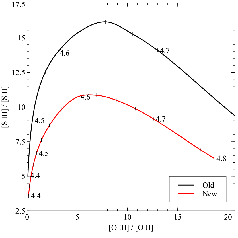
Figure 8: This shows the predicted ratios [S III] $\lambda$9530.6Å/[S II] $\lambda\lambda$ 6720Å and [O III] $\lambda$5006.84Å/[O II] $\lambda\lambda$ 3727Å where [S II] and [O II] are the summed intensities of the doublet. The model is of a blister H II region with Orion abundances and dust, ionized by various blackbodies with an ionization parameter of $\log U=-1.5$ (Osterbrock & Ferland, 2006). The blackbody temperatures were varied and the log of the value is indicated on the curves. The largest effect of the new recombination rate is to decrease [S III]/[S II] at a given [O III]/[O II].

The recombination rates recommended above have been adopted in the development version of Cloudy (Ferland et al., 2013) and will be used in the next release, now scheduled for early 2015. That version uses the general formula for DR suppression given by Nikolić et al. (2013). As recommended here, we do not suppress S${}^{2+}\rightarrow$S⁺ DR at photoionized plasma temperatures. These updates have a moderate effect on the spectrum. Cloudy includes an extensive suite of test cases that are used to validate its performance. This includes Active Galactic Nuclei, planetary nebulae, H II regions, and other classes of object. These tests show that the largest changes occur for H II regions ionized by cooler stars. The larger recombination rates increase the predicted [S II] / [S III], ratio by as much as 50% for late-type O stars. Figure 8 shows typical results. Changes in the [O II] and [O III] lines are modest and are caused by changes in the kinetic temperature resulting from changes in the S spectra. So the net effect is that, at a given [O II] / [O III] ratio, the [S II] / [S III] ratio is larger by $\sim 20-50$%.

This work was originally motivated by Henry et al. (2012), who documented “a Curious Conundrum Regarding Sulfur Abundances in Planetary Nebulae”. Uncertainties in the atomic database are a likely contributor to the conundrum. This pointed us towards the S${}^{2+}\rightarrow$S⁺ recombination rate, the only ion lacking modern DR calculations (e.g. missing from http://amdpp.phys.strath.ac.uk/tamoc/DR/). The revised DR rate derived here does not resolve the conundrum. We can only speculate as to its origin, but the ion state of S in an H II region, mainly single and doubly ionized, is lower than in a planetary nebula, with its hotter central star ionizing S to higher levels. The stellar SED was a major concern in the present study, and it seems likely that the SED for a planetary nebula nucleus might play a significant role in resolving the conundrum.

5 Conclusion

This paper suggests a way to make progress in solving the vexing and long-standing problem of finding good DR rates for the range of ions seen in astronomical observations. An observational program, combined with spectral modeling and a parallel effort in atomic theory, could make real progress in deriving DR rates for third and fourth row elements with well defined uncertainties. The elements of this program include the following:

Bootstrapping from astronomical observations of second-row elements. Section 2 outlined a novel method in which spectral models are used to match spectra produced by second-row elements, with good atomic data, to infer the rate for an ion on the third row. The key is that observations detect second-row ions which have a wider range of ionization potential than the species with the unknown rate. Section 3 shows that atomic theory can accommodate the empirical rate, and we illustrated the uncertainty which remains as we move away from the matching temperature. We concluded with a fit that can be used over all temperatures of physical interest. This procedure could be carried out for other species with adequate observations.

Insights from density dependencies. Astronomical observations of objects covering a range of densities can provide additional insights to the atomic structure. In the recombination process considered here the parent ion, S²⁺, has a ³P ground term. Our final fit to the DR rate predicts similar rate coefficients for the three $j=0,1,2$ levels within the ground term (Table 4), but this is not the case for results from other assumed atomic structures. Figure 6 shows that some predict a strong dependency on $j$. In those cases the total recombination rate will depend on the population of each $j$ level, which in turn depends on the electron density. So the recombination rate would have a strong density dependence if that structure was the correct one. Observations of nebulae that cover a range of densities could check whether this is the case, and could, absent the observations needed for the previous test, decide which curve in Figure 6 matches the observations.

References

- Abdel-Naby et al. (2012) Abdel-Naby, S. A., Nikolić, D., Gorczyca, T. W., Korista, K. T., & Badnell, N. R. 2012, A&A, 537, A40
- Aldrovandi & Pequignot (1973) Aldrovandi, S. M. V., & Pequignot, D. 1973, A&A, 25, 137
- Ali et al. (1991) Ali, B., Blum, R. D., Bumgardner, T. E., Cranmer, S. R., Ferland, G. J., Haefner, R. I., & Tiede, G. P. 1991, PASP, 103, 1182
- Asplund et al. (2009) Asplund, M., Grevesse, N., Sauval, A. J., & Scott, P. 2009, ARA&A, 47, 481
- Badnell (1991) Badnell, N. R. 1991, ApJ, 379, 356
- Badnell (2006a) —. 2006a, ApJS, 167, 334
- Badnell (2006b) —. 2006b, ApJ, 651, L73
- Badnell (2011) —. 2011, Computer Physics Communications, 182, 1528
- Badnell et al. (2003) Badnell, N. R., et al. 2003, A&A, 406, 1151
- Baldwin et al. (1991) Baldwin, J. A., Ferland, G. J., Martin, P. G., Corbin, M. R., Cota, S. A., Peterson, B. M., & Slettebak, A. 1991, ApJ, 374, 580
- Ferland & Savin (2001) Ferland, G., & Savin, D. W. 2001, Astronomical Society of the Pacific Conference Series, Vol. 247, Spectroscopic Challenges of Photoionized Plasmas
- Ferland (2003) Ferland, G. J. 2003, ARA&A, 41, 517
- Ferland et al. (1998) Ferland, G. J., Korista, K. T., Verner, D. A., Ferguson, J. W., Kingdon, J. B., & Verner, E. M. 1998, PASP, 110, 761
- Ferland et al. (2013) Ferland, G. J., et al. 2013, Rev. Mexicana Astron. Astrofis., 49, 137
- Henry et al. (2012) Henry, R. B. C., Speck, A., Karakas, A. I., Ferland, G. J., & Maguire, M. 2012, ApJ, 749, 61
- Jenkins (2009) Jenkins, E. B. 2009, ApJ, 700, 1299
- Kingdon & Ferland (1996) Kingdon, J. B., & Ferland, G. J. 1996, ApJS, 106, 205
- Kurucz (1979) Kurucz, R. L. 1979, ApJS, 40, 1
- Lanz & Hubeny (2003) Lanz, T., & Hubeny, I. 2003, ApJS, 146, 417
- Nahar (1995) Nahar, S. N. 1995, ApJS, 101, 423
- Nikolić et al. (2013) Nikolić, D., Gorczyca, T. W., Korista, K. T., Ferland, G. J., & Badnell, N. R. 2013, ApJ, 768, 82
- Nussbaumer & Storey (1983) Nussbaumer, H., & Storey, P. J. 1983, A&A, 126, 75
- Osterbrock & Ferland (2006) Osterbrock, D. E., & Ferland, G. J. 2006, Astrophysics of gaseous nebulae and active galactic nuclei
- Pauldrach et al. (2001) Pauldrach, A. W. A., Hoffmann, T. L., & Lennon, M. 2001, A&A, 375, 161
- Pauldrach et al. (1998) Pauldrach, A. W. A., Lennon, M., Hoffmann, T. L., Sellmaier, F., Kudritzki, R.-P., & Puls, J. 1998, in Astronomical Society of the Pacific Conference Series, Vol. 131, Properties of Hot Luminous Stars, ed. I. Howarth, 258
- Pequignot et al. (1978) Pequignot, D., Stasińska, G., & Aldrovandi, S. M. V. 1978, A&A, 63, 313
- Savin et al. (2012) Savin, D. W., et al. 2012, Reports on Progress in Physics, 75, 036901
- Schippers et al. (2004) Schippers, S., Schnell, M., Brandau, C., Kieslich, S., Müller, A., & Wolf, A. 2004, A&A, 421, 1185
- Sellmaier et al. (1996) Sellmaier, F. H., Yamamoto, T., Pauldrach, A. W. A., & Rubin, R. H. 1996, A&A, 305, L37+
- Simón-Díaz et al. (2006) Simón-Díaz, S., Herrero, A., Esteban, C., & Najarro, F. 2006, A&A, 448, 351
- Simón-Díaz & Stasińska (2008) Simón-Díaz, S., & Stasińska, G. 2008, MNRAS, 389, 1009
- van Hoof et al. (2004) van Hoof, P. A. M., Weingartner, J. C., Martin, P. G., Volk, K., & Ferland, G. J. 2004, MNRAS, 350, 1330
- Wen & O’Dell (1995) Wen, Z., & O’Dell, C. R. 1995, ApJ, 438, 784