Vertical Oscillations of Fluid and Stellar Disks

Abstract

A satellite galaxy or dark matter subhalo that passes through a stellar disk may excite coherent oscillations in the disk perpendicular to its plane. We determine the properties of these modes for various self-gravitating plane symmetric systems (Spitzer sheets) using the matrix method of Kalnajs. In particular, we find an infinite series of modes for the case of a barotropic fluid. In general, for a collisionless system, there is a double series of modes, which include normal modes and/or Landau-damped oscillations depending on the phase space distribution function of the stars. Even Landau-damped oscillations may decay slowly enough to persist for several hundred Myr. We discuss the implications of these results for the recently discovered vertical perturbations in the kinematics of solar neighborhood stars and for broader questions surrounding secular phenomena such as spiral structure in disk galaxies.

1 INTRODUCTION

In the $\Lambda$CDM cosmological paradigm, galactic disks are embedded in extended halos of dark matter, which are populated by satellite galaxies, star streams and dark matter subhalos. Inevitably, some of this halo substructure will pass through the disk, heating and thickening the disk and also triggering the development of secular phenomena such as spiral structure, bars, and warps.

In one of the earliest studies of disk heating, Toth & Ostriker (1992) calculated the energy that a passing satellite deposits in a stellar disk by assuming that the satellite gravitationally scatters individual disk stars. Their analysis, which was based on the Chandrasekhar (1943) dynamical friction formula, suggested that satellite infall could account for the thickness and velocity dispersion of galactic disks. On the other hand, the thinness and coldness of disks could be used to set constraints on the rate of satellite infall and hence the underlying cosmological model. Subsequent numerical experiments confirmed that satellites can in fact heat and thicken stellar disks, though perhaps not as efficiently as was suggested by Toth and Ostriker (see, for example Quinn et al. (1993); Walker et al. (1996); Huang & Carlberg (1997); Benson et al. (2004); Gauthier et al. (2006); Kazantzidis et al. (2008)).

The Toth & Ostriker (1992) calculation ignores two important effects. First, satellites are tidally disrupted by the gravitational field of the host galaxy, especially when their orbits take them into the central disk-dominated region. Second, disks can respond coherently to the gravitational field of a satellite. Hence, much of the energy that is transferred to the disk takes the form of large-scale perturbations such as warps in the outer disk (Quinn et al., 1993) or a tilt of the disk plane (Huang & Carlberg, 1997). Indeed satellites can change the morphology of a galaxy. Gauthier et al. (2006), Dubinski et al. (2008), and Kazantzidis et al. (2008) for example found that satellites and dark matter subhalos can provoke the formation of a bar and/or spiral structure. More recently, Purcell et al. (2011) suggested that the Sagittarius dwarf spheroidal galaxy might be responsible for the Milky Way’s bar and spiral structure.

The importance of coherent perturbations in disk-satellite interactions was stressed by Sellwood et al. (1998). They argued that a passing satellite transfers energy to the disk through the excitation of bending waves, which eventually decay through Landau damping. The upshot is that since the energy transfer from satellite to disk occurs through coherent perturbations disk heating is non-local.

Toomre (1966) derived the dispersion relation for bending waves in a stellar disk of zero thickness and uniform surface density. In general, these waves propagate in the disk plane with a group velocity that depends on the properties of the disk and the wavelength of the perturbation. Though Toomre’s analysis showed that a perturbation with a sufficiently short wavelength is susceptible to a buckling instability, he argued that this instability would be suppressed by the random motions of the stars in the vertical direction. These results were confirmed by Araki (1985) who studied wavelike perturbations of a stellar disk with finite thickness. In his equilibrium model, the surface density as well as the velocity dispersions in the vertical and horizontal directions are constant in space while the vertical structure is given by the isothermal plane solutions of Spitzer (1942) and Camm (1950). He found that the system avoided the buckling instability at all wavelengths provided the vertical velocity dispersion was greater than $0.293$ times the horizontal velocity dispersion. Araki (1985) also considered breathing modes, which correspond to compression and expansion of the disk perpendicular to and symmetric about the disk midplane. In this case, the system can undergo a Jeans instability.

Bending and breathing modes are the simplest modes in disklike systems, although they are no means only ones. In order to explore vertical perturbations in more detail, one can ignore variations in the horizontal direction. Antonov (1971); Kalnajs (1973); Fridman et al. (1984), for example, considered strictly vertical perturbations of a homogeneous slab and found an infinite double series of normal modes. On the other hand Mathur (1990) and Weinberg (1991) investigated vertical oscillations in a variant of the Spitzer sheet where the stellar energy distribution is truncated (the lowered Spitzer sheet) and were able to identify only a handful of normal modes.

Our aim is to carry out a comprehensive study of vertical oscillations in stellar and gaseous disks. In particular we extend the analysis of Mathur (1990) and Weinberg (1991) to Landau-damped oscillations by using the matrix method of Kalnajs (1977) and complex analysis techniques from Landau (1946) and Lynden-Bell (1962). We begin by calculating the normal modes of a gaseous disk, which serves as a warm-up to the the more complex collisionless case. We then discuss normal modes of the homogeneous slab. Finally we turn to the original (untruncated) and lowered Spitzer sheets. In both cases, we identify a double series of Landau-damped oscillations. We contend that these “modes”, combined with the normal modes found in Mathur (1990) and Weinberg (1991), are analogous to the double series of modes of the homogeneous slab. Since we only consider vertical motions we cannot directly address the question of how modes propogate in the disk plane as was done in Araki (1985) (see, also a brief discussion in Weinberg (1991)) though we do gain a more complete understanding of vertical modes and Landau-damped oscillations.

The primary motivation for this work comes from recent observations of vertical phase space structures in the kinematics of disk stars in the solar neighborhood of the Milky Way. These observations come free three surveys: the Sloan Extension for Galactic Understanding and Exploration (SEGUE; Yanny et al. (2009)), the RAdial Velocity Experiment (RAVE; Steinmetz et al. (2006)), and the LAMOST Experiment for Galactic Understanding and Exploration (LEGUE; Deng et al. (2012)). These surveys provide full six-dimensional phase space information for tens of thousands of stars within a few kiloparsecs of the Sun. Recently, several groups have detected vertical bulk motions using data from these surveys (Widrow et al., 2012; Williams et al., 2013; Carlin et al., 2013), which appear to take the form of compression and expansion of the stellar disk. In addition, Widrow et al. (2012) and Yanny & Gardner (2013) found evidence for wavelike North-South asymmetries in the number counts of solar neighborhood stars.

Velocity and number density perturbations normal to the Galactic midplane can result from satellite-disk interactions (Widrow et al., 2012; Gómez et al., 2013; Widrow et al., 2014). Gómez et al. (2013), for example, used N-body experiments to show that a Sagittarius-like dwarf with a mass of $10^{10.5}-10^{11}\,M_{\odot}$ could produce density perturbations of the same amplitude as was seen in Widrow et al. (2012) and Yanny & Gardner (2013). Simulations by Feldmann & Spolyar (2015) showed that lower mass ($10^{8}-10^{9}\,M_{\odot}$) satellites produce subtle features in the bulk velocity field of the disk that might be observed in the next generation of astrometric surveys such as Gaia (Perryman et al., 2001).

The bar and spiral structure of the Milky Way can also perturb the velocity distribution of stars in the disk and might therefore be responsible, at least in part, for the observations described above. In particular Dehnen (2000), Fux (2001) and Bovy (2010) showed that a resonant interaction between the Milky Way’s bar and stars in the solar neighborhood might be responsible for the Hercules stream, a group of co-moving stars whose bulk velocity is offset from that of the local standard of rest. Faure et al. (2014) used test-particle simulations to study the response of disk stars to a spiral potential perturbation and showed that spiral structure could generate vertical bulk motions in the disk akin to what has been observed in the SEGUE, RAVE, and LEGUE surveys. Debattista (2014) carried out a fully self-consistent N-body simulation of a spiral galaxy and came to similar conclusions. Essentially, a spiral arm causes compression and expansion as it sweeps through the disk.

Of course, since satellites have also been implicated in triggering the formation of bars and spiral structure, it may be difficult to disentangle perturbations that come directly from a disk-satellite interaction and perturbations due to structures in the disk, which themselves were the result of passing satellites. Widrow et al. (2014) followed the evolution of bending and breathing modes in the Gauthier et al. (2006) simulation, where the disk was subjected to the continual perturbations of a substructure-filled halo. Bending and breathing modes appear at early times as subhalos churn up the disk. The formation of a bar, which occurs at about $5\,{\rm Gyr}$, is clearly triggered by substructure-disk interactions and it may well be that the breathing mode perturbations are the mechanism by which this occurs. Moreover, at late times the bar itself maintains both bending and breathing modes, especially in the inner parts of the galaxy.

A second and more academic purpose for this work is to explore normal modes and Landau damping in self-consistent one-dimensional systems. In the usual textbook explanation of the Jeans instability one considers perturbations of a spatially homogeneous mass distribution. In the case of a fluid, one assumes that the sound speed is constant while for a collisionless system, one assumes a Maxwellian velocity distribution with constant velocity dispersion. In either case, one must confront the conundrum that the unperturbed gravitational potential $\psi_{0}$ is ill-defined. By symmetry, $\boldsymbol{\nabla}\psi_{0}=0$ in a homogeneous system whereas Poisson’s equation implies $\nabla^{2}\psi_{0}=4\pi G\rho_{0}$. These two equations are inconsistent. The Jeans swindle, wherein one makes the ad hoc assumption that Poisson’s equation applies only to perturbed quantities, provides a way forward (see Binney & Tremaine (2008) for a more detailed discussion). The linearized equations are then solved by making the ansatz that the perturbed density and potential vary harmonically in space and time. In both the fluid and collisionless cases a perturbation whose wavelength is longer than the Jeans length grows exponentially. A perturbation in a fluid whose wavelength is less than the Jeans length oscillates as sound waves. On the other hand, a short wavelength perturbation in a collisionless system undergoes Landau damping and rapidly decays. In the models considered here, the density is concentrated in the midplane and the Poisson equation can be solved without resorting to the Jeans swindle.

The outline of the paper is as follows: In Section 2 we find the normal modes for an isothermal plane-symmetric fluid. In Section 3, we derive normal and Landau-damped oscillations for the three examples of collisionless systems mentioned above. In Section 4, we present results from a simulations of a one-dimensional system that exhibits damping in a perturbed Spitzer sheet. We conclude in Section 5 with a summary and discussion of our results and some thoughts on further directions for this line of research. Three appendices provide mathematical details for some of our calculations.

2 LINEAR PERTURBATIONS OF AN ISOTHERMAL ONE-DIMENSIONAL FLUID

In this section and the ones that follow, we consider the vertical perturbations of plane symmetric systems. The idea of treating a galactic disk as a plane symmetric system can be traced to the seminal paper by Oort (1932), wherein the motions of stars perpendicular to the Galactic midplane were used to estimate the vertical force and mass distribution in the solar neighborhood. Spitzer (1942) derived an equilibrium model for a self-gravitating, plane-symmetric system of stars under the assumption that the stellar velocity dispersion is constant with height above the midplane. His derivation is based on the Jeans equations (i.e., moments of the collisionless Boltzmann equation) and is therefore akin to the derivation of the equilibrium fluid model considered in this section. Camm (1950) solved for the equilibrium distribution function, which provides the starting point for our analysis in Section 3. In what follows, we refer to these models collectively as Spitzer sheets.

We consider linear perturbations in a simple self-gravitating barotropic fluid. For an analysis of perturbations in a multiphase, magnetized model of the interstellar medium see Walters & Cox (2001). A fluid with density $\rho$, velocity $v$, pressure $p$, and gravitational potential $\psi$ obeys the continuity, Euler, and Poisson equations. For a plane symmetric system, these equations become

$$\frac{\partial\rho}{\partial t}+\frac{\partial}{\partial z}\left(\rho v\right)=0$$ (1)

$$\frac{\partial v}{\partial t}+v\frac{\partial v}{\partial z}=-\frac{1}{\rho}\frac{\partial p}{\partial z}-\frac{\partial\psi}{\partial z}$$ (2)

$$\frac{\partial^{2}\psi}{\partial z^{2}}=4\pi G\rho$$ (3)

where we choose our coordinate system so that the $z$-axis is normal to the symmetry plane. We assume that the fluid has an equation of state $p=p\left(\rho\right)$ and constant sound speed $v_{s}\equiv\left(dp/d\rho\right)^{1/2}$.

We write $\rho$, $v$, $p$, and $\psi$ as the sum of an equilibrium solution and a linear perturbation, e.g.,

$$\rho=\rho_{0}\left(z\right)+\rho_{1}\left(z,t\right)~{}.$$ (4)

For the equilibrium solution, $v_{0}=0$ and the continuity equation is satisfied automatically while the Euler and Poisson equations are solved by the following density-potential pair:

$$\psi_{0}\left(z\right)=2v_{s}^{2}\ln\left(\cosh\left(z/z_{0}\right)\right)$$ (5)

and

$$\rho_{0}\left(z\right)=\rho_{c}\,{\rm sech}^{2}\left(z/z_{0}\right)$$ (6)

where $z_{0}\equiv v_{s}/\left(2\pi G\rho_{c}\right)^{1/2}$ and $\rho_{c}$ is the density in the midplane (Spitzer, 1942; Camm, 1950).

In what follows, we use a system of units in which $z_{0}=v_{s}=G=1$ and $\rho_{c}=1/2\pi$. The linearized equations are

$$\frac{\partial\rho_{1}}{\partial t}+\frac{\partial}{\partial z}\left(\rho_{0}v_{1}\right)=0$$ (7)

$$\rho_{0}\frac{\partial v_{1}}{\partial t}=-\frac{\partial\rho_{1}}{\partial z}-\rho_{1}\frac{\partial\psi_{0}}{\partial z}-\rho_{0}\frac{\partial\psi_{1}}{\partial z}$$ (8)

$$\frac{\partial^{2}\psi_{1}}{\partial z^{2}}=4\pi\rho_{1}~{}.$$ (9)

To search for modes, we assume that the first-order quantities are proportional to $\exp{(-i\omega t)}$ (e.g., $\rho_{1}\left(z,\,t\right)=\exp\left({-i\omega t}\right)\tilde{\rho_{1}}(z)$) and combine the continuity and Euler equations to arrive at a single equation for $\tilde{\rho_{1}}$:

$$\omega^{2}\tilde{\rho_{1}}=-\frac{d^{2}\tilde{\rho_{1}}}{dz^{2}} -\frac{d\tilde{\rho_{1}}}{dz}\frac{d\psi_{0}}{dz}$$ (10)

$$-\tilde{\rho_{1}}\frac{d^{2}\psi_{0}}{dz^{2}}-\frac{d\rho_{0}}{dz}\frac{d\tilde{\psi_{1}}}{dz}-\rho_{0}\frac{d^{2}\tilde{\psi_{1}}}{dz^{2}}~{}.$$ (11)

For a homogeneous system, the fourth term on the right-hand side is zero while the second and third terms are ignored by implementing the Jeans swindle (Binney & Tremaine, 2008). We then assume a sinusoidal spatial dependence for the perturbation ($\tilde{\rho}_{1},~{}\tilde{\psi}_{1}\propto\exp{(ikz)}$) and use the first-order Poisson equation to arrive at the dispersion relation

$$\omega^{2}=v_{s}^{2}\left(k^{2}-k_{J}^{2}\right)=k^{2}-2$$ (12)

where $k_{J}\equiv\left(4\pi G\rho_{c}/v_{s}^{2}\right)^{1/2}=2^{1/2}$ is the Jeans wavenumber. For $k<k_{J}$ (long wavelength perturbations) $\omega$ is imaginary signaling an instability with growth rate $\alpha=\left(2-k^{2}\right)^{1/2}$. On the other hand, for $k>k_{J}$ perturbations oscillate with frequency $\omega=\left(k^{2}-2\right)^{1/2}$.

To study linear perturbations of the Spitzer sheet we use the Kalnajs matrix method and write $\tilde{\rho}_{1}$ and $\tilde{\psi}_{1}$ in terms of a biorthonormal basis (Kalnajs, 1971, 1977; Binney & Tremaine, 2008):

$$\tilde{\psi}_{1}\left(z\right)=\sum_{j}c_{j}\psi_{j}\left(z\right)~{}~{}~{}~{}~{}~{}\tilde{\rho}_{1}\left(z\right)=\sum_{j}c_{j}\rho_{j}\left(z\right)$$ (13)

where

$$\frac{d^{2}\psi_{j}}{dz^{2}}=4\pi\rho_{j}$$ (14)

and

$$\int_{-\infty}^{\infty}dz\,\psi_{j}^{*}(z)\rho_{k}(z)=-\delta_{jk}~{}.$$ (15)

We multiply Eq. 10 by $-\psi_{j}$ and integrate with respect to $z$ from $-\infty$ to $\infty$ to obtain a matrix equation of the form

$$\omega^{2}c_{j}=\sum_{k}M_{jk}c_{k}~{}.$$ (16)

Evidently, the eigenvalues of ${\bf M}$ are the squares of the mode frequencies.

For the calculation at hand we use the basis introduced in Araki (1985):

$$\psi_{j}\left(z\right)=N_{j}P_{j}(u)$$ (17)

and

$$\rho_{j}\left(z\right)=-N_{j}\frac{j\left(j+1\right)}{4\pi}\left(1-u^{2}\right)P_{j}(u)$$ (18)

where $u={\rm tanh}(z)$, $P_{j}$ are Legendre polynomials, and $N_{j}\equiv\left(2\pi\left(2j+1\right)/{j\left(j+1\right)}\right)^{1/2}$ are normalization constants. The matrix elements $M_{jk}$ can be calculated analytically (see Appendix A). Note that $M_{jk}$ is nonzero if and only if $j=k-2,\,k,$ or $k+2$. The matrix therefore separates into two independent matrices, one where $j$ and $k$ are both even and the other where $j$ and $k$ are both odd. The physical implication is that modes have definite parity, a property that follows from the symmetry of the equilibrium system under the transformation $z\to-z$.

The eigenvalues and eigenvectors for these sparse matrices are found using the software package LAPACK (Anderson et al., 1992). The frequencies $\omega_{n}$ and eigenfunctions for the lowest eight modes are given in Table 1 and Figure 1. The eigenfunction label $n$ corresponds to the number of nodes in the density profile. Note that the $n=1$ mode, which has zero frequency, corresponds to a shift in the system as a whole.

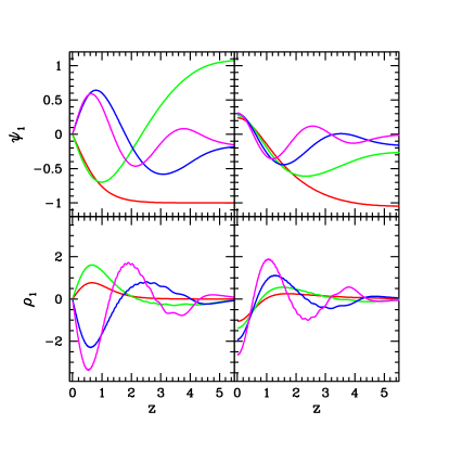
Figure 1: Normal modes of the fluid Spitzer sheet. Panels on the left show the potential (top) and density (bottom) for the odd parity modes with $n=1$ (red curve), $n=3$ (green), $n=5$ (blue) and $n=7$ (magenta). Panels on the right show the even parity modes $n=2$ (red curve), $n=4$ (green), $n=6$ (blue) and $n=8$ (magenta).

odd modes		even modes
$n$	$\omega_{n}$	$n$	$\omega_{n}$
1	0	2	1.129
3	1.522	4	2.180
5	3.138	6	4.373
7	5.976	8	7.865

Table 1: Frequencies, in units of where $v_{s}=z_{0}=1$ for the first four even and first four odd modes.

3 COLLISIONLESS SYSTEMS

3.1 Formalism

The dynamics of a collisionless, plane symmetric system is described by the collisionless Boltzmann and Poisson equations in one dimension. We follow the formalism found in Mathur (1990) and Weinberg (1991) in which the collisionless Boltzmann equation is written in terms of angle-action variables (see, also Binney & Tremaine (2008)). For an alternate approach based on Jeans equations, see Louis (1992). A particle in a time-independent potential, $\psi_{0}(z)$ executes periodic motion with constant energy $E=v^{2}/2+\psi_{0}\left(z\right)$, period $T(E)$, and maximum excursion from the midplane $z_{\rm max}$ where $\psi_{0}\left(z_{\rm max}\right)=E$. We can therefore introduce the angle-action variables $\left(\theta,\,E\right)$ where $\theta$ is defined so that $dt=T(E)d\theta/2\pi$ and $\theta=0$ corresponds to $\left(z,\,v\right)=\left(-z_{\rm max},\,0\right)$.

As before, we write the density and potential, along with the distribution function, as the sum of an equilibrium solution and a linear perturbation. For example

$$f\left(E,\,\theta,\,t\right)=f_{0}\left(E\right)+f_{1}\left(E,\,\theta,\,t\right)~{}.$$ (19)

The linearized collisionless Boltzmann and Poisson equations are then

$$\frac{\partial f_{1}}{\partial t}+\frac{2\pi}{T(E)}\frac{\partial f_{1}}{\partial\theta}-\frac{2\pi}{T(E)}\frac{\partial f_{0}}{\partial E}\frac{\partial\psi_{1}}{\partial\theta}=0$$ (20)

and

$$\frac{\partial^{2}\psi_{1}}{\partial z^{2}}=4\pi G\int dv\,f_{1}~{}.$$ (21)

Note that the Newtonian potential that appears in the collisionless Boltzmann equation includes contributions from both the system and any external perturbations while $f_{1}$ refers only to the system.

Since particle orbits are periodic in $\theta$ we can expand each of the first-order quantities in a Fourier series, e.g.,

$$f_{1}\left(E,\,\theta,t\right)=\sum_{n=-\infty}^{\infty}f_{n}\left(E,\,t\right)e^{in\theta}~{}.$$ (22)

Eq. 20 is satisfied for each Fourier component:

$$\frac{\partial f_{n}}{\partial t}+\frac{2\pi in}{T(E)}f_{n}-\frac{2\pi in}{T(E)}\frac{\partial f_{0}}{\partial E}\psi_{n}=0~{}.$$ (23)

The temporal Fourier transform of $f_{n}$ is

$$\tilde{f}_{n}\left(E,\,\omega\right)=\int_{0}^{\infty}dt\,f_{n}\left(E,\,t\right)e^{i\omega t}$$ (24)

and similarly for $\psi_{n}$. In writing $\tilde{f}_{n}$, we have assumed that $f_{n}=0$ for $t<0$ and that there exists a real number $\gamma>0$ such that $\int dt\,{\rm exp}\left(-\gamma t\right)f_{n}(t)$ converges. The latter condition insures the existence of the inverse Fourier transform (Binney & Tremaine (2008) – see Eq. 35 below. We multiply Eq. 23 by ${\rm exp}\left(i\omega t\right)$ and integrate over $t$. The first term is handled by an integration by parts and we obtain an algebraic equation for $\tilde{f}_{n}$, which can be written as

$$\tilde{f}_{n}\left(E,\,\omega\right)=\frac{df_{0}}{dE}\frac{n\Omega(E)\tilde{\psi}_{n}\left(E,\,\omega\right)}{n\Omega(E)-\omega}$$ (25)

where $\Omega(E)\equiv 2\pi/T(E)$ is the orbital frequency for a particle with energy $E$.

As in the fluid case, we decompose the density and potential in terms of a biorthonormal basis. Let $\psi_{1}^{s}$ be the linear perturbation to the potential due to the system itself and $\psi_{1}^{e}$ be the linear external potential (if one exists). For the system, we have

$$\tilde{\psi}_{1}^{s}\left(z,\,\omega\right)=\sum_{j=1}^{\infty}c_{j}\left(\omega\right)\psi_{j}\left(z\right)$$ (26)

and

$$\tilde{\rho}_{1}^{s}=\int dv\,f_{1}=\sum_{j=1}^{\infty}c_{j}\left(\omega\right)\rho_{j}\left(z\right)$$ (27)

where the potential-density pair $\left(\psi_{j},\,\rho_{j}\right)$ satisfy Eqs. 13-15. Likewise, for the external potential, we have

$$\tilde{\psi}_{1}^{e}\left(z,\,\omega\right)=\sum_{j=1}^{\infty}d_{j}\left(\omega\right)\psi_{j}\left(z\right)~{}.$$ (28)

We then write $\psi_{j}$ as a Fourier series

$$\psi_{j}(z)=\sum_{n=-\infty}^{\infty}\psi_{jn}(E)e^{in\theta}$$ (29)

where

$$\psi_{nj}(E)=\frac{1}{2\pi}\int_{0}^{2\pi}d\theta\,\psi_{j}\left(z\left(E,\,\theta\right)\right)e^{-in\theta}~{}.$$ (30)

We now use Eq. 25 and the expansions defined above to write the Poisson equation as follows:

$$\frac{1}{4\pi G}\frac{d^{2}\tilde{\psi}_{1}}{dz^{2}} =\sum_{j=1}^{\infty}c_{j}\rho_{j}$$

$$=\sum_{n=-\infty}^{\infty}\int dv\frac{df_{0}}{dE}\frac{n\Omega\tilde{\psi}_{n}}{n\Omega-\omega}e^{in\theta}$$ (31)

where $\tilde{\psi}_{n}=\tilde{\psi}_{n}^{s}+\tilde{\psi}_{n}^{e}=\sum_{j}\left(c_{j}+d_{j}\right)\psi_{jn}$.

We multiply this equation by $-\psi_{j}(z)$ and integrate over $z$ to arrive at a matrix equation the expansion coefficients $c_{j}$:

$$c_{j}\left(\omega\right)=M_{jk}\left(\omega\right)\left(c_{k}\left(\omega\right)+d_{k}\left(\omega\right)\right)$$ (32)

where

$$M_{jk}\left(\omega\right)=-4\pi\sum_{n=1}^{\infty}\int dE\frac{df_{0}}{dE}\frac{\Omega\psi_{jn}\psi_{kn}}{\Omega^{2}-\omega^{2}/n^{2}}$$ (33)

(Mathur, 1990; Weinberg, 1991). Note that in deriving Eq. 33, we have combined positive and negative values of $n$ and also omitted the $n=0$ term as its contribution to the sum is zero. The matrix ${\bf M}$, which is sometimes referred to as the polarization matrix (Binney & Tremaine, 2008), describes the response of the system to the total perturbing potential (system plus external). We can rewrite Eq. 32 as an explicit equation for the $c_{j}$:

$$c_{j}\left(\omega\right)=\sum_{k}R_{jk}\left(\omega\right)d_{k}\left(\omega\right)$$ (34)

where ${\bf R}\equiv\left({\bf I-M}\right)^{-1}{\bf M}$ describes the response of the system to an external potential.

The time-dependent response of the system is determined by calculating the inverse Fourier transform of $c_{j}$:

$$c_{j}\left(t\right) =\frac{1}{2\pi}\int_{i\gamma-\infty}^{i\gamma+\infty}d\omega\,c_{j}\left(\omega\right)e^{-i\omega t}$$ (35)

$$=-i\sum_{r}c_{j,r}\left(\omega_{r}\right)e^{-i\omega_{r}t}$$ (36)

where $\omega_{r}$ are the poles of the function $c_{j}\left(\omega\right)$. These poles occur at the poles of the response matrix ${\bf R}$ or equivalently, where either ${\rm det}({\bf M})$ is singular or ${\rm det}\left({\bf I}-{\bf M}\right)=0$. The second of these conditions is equivalent to the eigenvalue equation

$$c_{j}\left(\omega\right)=\sum_{k}M_{jk}\left(\omega\right)c_{k}\left(\omega\right)~{}.$$ (37)

Our goal is therefore to find frequencies $\omega_{m}$ such that one of the eigenvalues of ${\bf M}$ is equal to unity. The corresponding functions $\psi_{1}^{s}\left(z,\,\omega_{m}\right)$ and $\rho_{1}^{s}\left(z,\,\omega_{m}\right)$ are then the potential-density pairs for either normal modes, when ${\rm Im}\left(\omega_{m}\right)=0$ or Landau-damped oscillations, when ${\rm Im}\left(\omega_{m}\right)<0$.

3.2 Homogeneous slab of stars

We first determine the normal modes of the spatially homogeneous slab (Antonov, 1971; Kalnajs, 1973; Fridman et al., 1984), where the distribution function for the equilibrium system is given by

$$f_{0}(E)=\begin{cases}f_{c}\left(1-E/\sigma^{2}\right)^{-1/2}&{\rm for}~{}~{}0<E<\sigma^{2}\\ 0&{\rm otherwise}~{}.\end{cases}$$ (38)

The density is equal to the constant $\rho_{c}=2^{1/2}\pi\sigma f_{c}$ for $|z|<\left(\sigma^{2}/2\pi G\rho_{c}\right)^{1/2}$ and zero otherwise. All particles execute simple harmonic motion about the midplane with frequency $\Omega_{c}=\left(4\pi G\rho_{c}\right)^{1/2}$. We choose units akin to those used in the previous section, namely $\sigma=G=1$ and $\rho_{c}=1/2\pi$. The edge of the slab is then at $z=\pm 1$ and $\Omega_{c}=2^{1/2}$.

Following Kalnajs (1973) we use the biorthonormal basis to describe the density and potential inside the slab:

$$\psi_{j}(z)=N_{j}\left(P_{j+1}(z)-P_{j-1}(z)\right)$$ (39)

and

$$\rho_{j}(z)=-\frac{N_{j}}{4\pi}\frac{j\left(j+1\right)}{1-z^{2}}\left(P_{j+1}(z)-P_{j-1}\right)$$ (40)

where $N_{j}=\left(2\pi/\left(2j+1\right)\right)^{1/2}$. In fact, $\left(\psi_{j},\,\rho_{j}\right)$ are the normal modes of the system. We see that the density and potential have even parity when $j$ is odd and vice versa. Furthermore, when $j$ is odd, there are $\left(j+1\right)/2$ distinct modes (Kalnajs, 1973). We label the frequencies for these modes $\omega_{j,k}$ where $k=1,\,3\dots\left(j+1\right)/2$. Likewise, when $j$ is even, there are $\left(j+2\right)/2$ modes. For example, there is a single mode with $j=1$: $\psi_{1}=\left(3N_{1}/2\right)\left(z^{2}-1\right)$, $\rho_{1}=3N_{1}/4\pi$, and $\omega_{1,1}=6^{1/2}=1.73\Omega_{c}$ (Antonov, 1971; Kalnajs, 1973; Fridman et al., 1984). The distribution function for this mode is

$$f_{1}\left(z,\,v\right)=\frac{3N_{1}E}{2}\,\frac{df_{0}}{dE}\,\frac{\cos{2\theta}}{2-\omega^{2}/4}$$ (41)

(see Appendix B). The frequencies of the $j\leq 5$ modes are depicted in Figure 2; numerical values can be found in Kalnajs (1973).

Self-consistency requires $\rho_{1}=\int dv\,f_{1}$. Formally, this integral is infinite because of the strong divergence of $df_{0}/dE$ as $E\to 1$. To handle this divergence we consider a family of functions $f_{\lambda}(E)$ that are continuous, that vanish as $E\to\infty$ and that approach Eq. 38 in the limit $\lambda\to\infty$. We can then perform an integration by parts and afterwards let $\lambda\to\infty$ (see for example, Fridman et al. (1984)). As shown in Appendix B, this procedure leads to the required relation between $\rho_{1}$ and $f_{1}$. A similar trick can be used to evaluate the matrix elements in Eq. 33 where we can write

$$M_{jk}\left(\omega\right)=-\sum_{n}\frac{4\pi\Omega_{c}}{\Omega_{c}^{2}-\omega^{2}/n^{2}}\,\int dE\,f_{0}\frac{d}{dE}\left(\psi_{jn}\psi_{kn}\right).$$ (42)

The function $f_{0}$ has an integrable singularity at $E=1$ and the matrix elements can be calculated numerically. In doing so, we find that ${\bf M}$ is indeed diagonal, a result that Kalnajs (1973) showed using various relations between Legendre polynomials and hypergeometric functions.

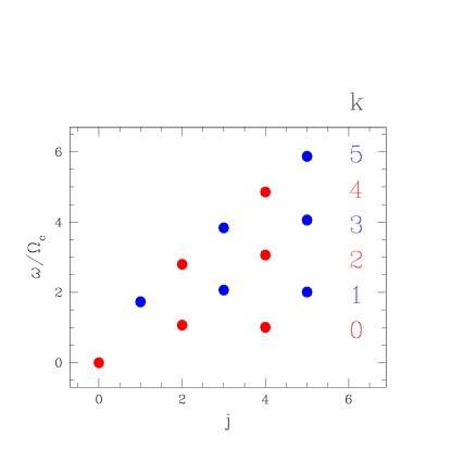
Figure 2: Frequencies for normal modes of the homogeneous stellar slab. The dots give the frequencies from Kalnajs (1973) for different values of the eigenvalues $j$ and $k$. Red dots are for even $j$ and correspond to modes where the density and potential have odd parity under $z\to-z$. Blue does are for even parity (odd $j$) modes. Modes in the same column have the same density and potential but different phase space distribution functions.

In Figure 3 we show the density and potential pairs for the even parity modes with $j=1,\,3,\,5$. The case $j=1$ is a breathing mode in which the density within the slab depends on $t$ but not $z$, while the boundaries of the slab move in and out accordingly. The distribution functions for the six distinct modes with these values of $j$ are shown in Figure 4. Modes in the same row have frequencies that cluster about $\left(j+1\right)\Omega_{c}$, as in Figure 2. For example, the three modes along the bottom row have frequencies from left to right of $\omega/\Omega_{c}=1.73,2.07,2.01$. Particles make roughly half an orbit in the time it takes the system to execute a single mode oscillation of this type. The frequencies for the two modes in the middle row are $\omega/\Omega_{c}=3.83,\,4.06$ so that particles make roughly one quarter of an orbit during one oscillation period. Modes in the same column have the same density profile and potential since they have the same eigenvalue $j$.

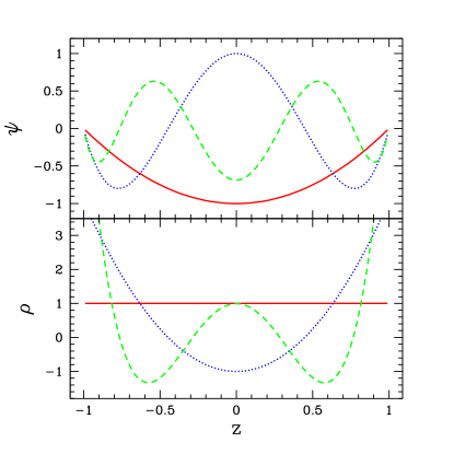
Figure 3: Even parity normal modes of the homogeneous slab. The linear potential (top panel) and density (bottom panel) are shown as a function of $z$ for $j=1$ (red/solid), $j=3$ (blue/dotted) and $j=5$ (green/dashed).

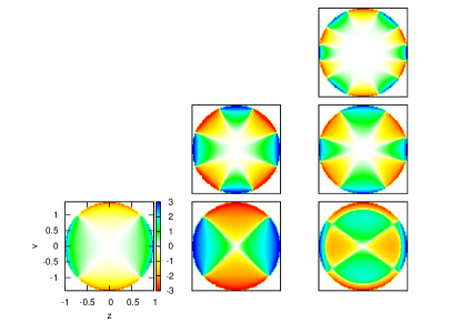
Figure 4: Distribution functions for even parity modes of the homogeneous slab with $j=1,\,3,\,5$. The arrangement of the panels is the same as the arrangement of the blue dots in Figure 2. Thus, the three modes along the bottom row have, from left to right, $j=1,\,3,$ and $5$ and $\omega\simeq 1.73,\,2.07,$ and $2.01$. The three modes along the right column all have $j=5$ and have a density profile and potential given by the green/dashed curves in Figure 3.

3.3 Linear perturbations of the stellar Spitzer sheet

In a collisionless system, oscillations that are in resonance with any of the particles in the distribution will decay via Landau damping whereby coherent energy in the oscillations is transferred to energy in random particle motion. The homogeneous slab is a special example where all particles have the same orbital frequency $\Omega_{c}$. Since the mode frequencies are all slightly off resonance there is no Landau damping, at least not formally.

In this section we consider the stellar Spitzer sheet where the distribution function is

$$f_{0}(E)=f_{c}e^{-E/\sigma^{2}}~{}.$$ (43)

The density and potential have the same form as in the fluid case (Eqs. 5 and 6) but with $v_{s}$ replaced by $\sigma$ and $f_{c}=\rho_{c}/\left(2\pi\sigma^{2}\right)^{1/2}$. As before, we choose units in which $G=z_{0}=\sigma=1$. In these units, the orbital frequencies range from $\Omega(E)\to\Omega_{c}=2^{1/2}$ for $E\to 0$ to $\Omega(E)\to 0$ for $E\to\infty$. Thus, coherent oscillations with frequency $\omega$ will be in resonance with particles whose orbital frequencies are $\Omega_{n}=\omega/n$ where $n=n_{\rm min},\,n_{\rm min}+1,\,\dots$ and $n_{\rm min}={\rm Int}(\Omega_{c}/\omega)$. This point is illustrated in Figure 5. The line segments in the middle portion of the diagram show the range in orbital frequencies and higher harmonics for the Spitzer sheet. The dots along the top portion of the diagram show the same for the homogeneous slab. The modes of the homogeneous slab are all off-resonance, that is, reside in the gaps between the dots. No such gaps exist in the case of the Spitzer sheet. The implication is that all coherent oscillations of the Spitzer sheet are damped.

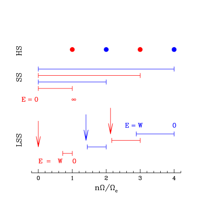
Figure 5: Range of allowed frequencies for orbits of stars and their harmonics in the lowered Spitzer sheet (LSS), the Spitzer sheet of Spitzer (1942) and Camm (1950) (SS) and the homogeneous plane (HS). The left-most horizontal bar in the row marked LSS shows the range of allowed frequencies for orbits in the lowered Spitzer sheet with $W=2$. The blue bar immediately to the right of this shows the frequencies for the second harmonics of these orbits, and so on. The vertical arrows mark the positions of the modes found by Mathur (1990) and Weinberg (1991). The frequency ranges for the Spitzer sheet are displayed in the same way while for the homogeneous plane all particles orbit at the same frequency. Odd parity modes and frequencies are shown in red while even parity modes and frequencies are shown in blue.

We also consider the lowered Spitzer sheet, which provides a link between the the homogeneous slab and the Spitzer sheet. This model the one-dimensional analog of the lowered isothermal sphere or King model and has a distribution function that is given by

$$f_{0}(E)=\begin{cases}f_{W}\left(e^{-E/\sigma^{2}}-e^{-W/\sigma^{2}}\right)&0<E<W\\ 0&{\rm otherwise}~{}.\end{cases}$$ (44)

With $\sigma=1$ and

$$f_{W}=\sigma^{-1}\left(\left(2\pi\right)^{3/2}{\rm erf}\left(y_{0}\right)-2^{5/2}\pi y_{0}e^{-y_{0}^{2}}\right)^{-1}$$ (45)

where $y_{0}\equiv W^{1/2}/\sigma$, the density in the midplane is $\rho_{c}=1/2\pi$ and the maximum orbital frequency is $\Omega_{c}=2^{1/2}$ (See Appendix C2 for details). For finite $W$ there is a lower bound on the particle frequencies: $\Omega_{\rm min}\equiv\Omega(W)$.

The horizontal line segments in the lower portion of Figure 5 show the range in frequencies and higher harmonics for the case $W=2$. We see that there are no resonant particles for $0<\omega\la 0.72\,\Omega_{c}$. Mathur (1990) and Weinberg (1991) refer to this range in frequency as the principal gap. Likewise, there are no particles with $\Omega_{c}<\omega\la 1.45\,\Omega_{c}$ (the first gap).

As discussed above, our aim is to find values of $\omega$ for which one of the eigenvalues of the matrix ${\bf M}$ is equal to one. Mathur (1990) and Weinberg (1991) restrict their search for modes to real values $\omega$ that reside in the frequency gaps. In doing so, they avoid any potential singularities in the energy integrals necessary for calculating the matrix elements. The vertical arrows in Figure 5 indicate the positions of the modes found by the method outlined in Mathur (1990) and Weinberg (1991). Note that apart from the $\omega=0$ mode, the frequencies are slightly less than $n\Omega_{\rm min}$.

Next we consider complex values of $\omega$. Recall that the Fourier transform $\tilde{f}_{n}$ and hence the matrix elements $M_{jk}$ are defined for ${\rm Im}(\omega)>0$. In this regime, the energy integrals in Eq. 33 can be calculated by a straightforward numerical integration since the singularity in the integrand occurs in the lower half of the complex $E$ plane and is avoided as one integrates along the real $E$ axis.

To explore solutions with ${\rm Im}(\omega)\leq 0$ we analytically continue ${\bf M}$ into this region of the complex $\omega$ plane. To see how this works we define ${\cal M}_{jk}\left(\omega_{R},\,\omega_{I};\lambda\right)\equiv M_{jk}\left(\omega_{R}+i\lambda\omega_{I}\right)$ to be a function of the real variable $\lambda$ with $\omega_{R}$ and $\omega_{I}$ taken to be positive constants. The analytic continuation of $M_{jk}$ will have the property that ${\cal M}_{jk}$ is a continuous function of $\lambda$. When $\lambda$ changes from positive to negative values, the singularity in the energy integral crosses from the lower half of the complex energy plane to the upper half. Thus, if $M_{jk}$ is to be continous when this happens, the integration contour for the energy integral must deformed so that the it always remains above the singularity. This deformed contour is analogous to the so-called Landau contour used to carry out the velocity-space integral in the usual derivation of Landau damping for a homogeneous system (Landau, 1946; Lynden-Bell, 1962; Binney & Tremaine, 2008). We then have two contributions to the energy integrals in Eq. 33, one from the principal part of the integral, and the other from the residue due to the singularity at $\Omega(E)=\omega/n$. That is, each term of the sum in Eq. 33 becomes

$$-4\pi{\cal P}\int dE\,\frac{\Omega\psi_{jn}\psi_{kn}}{\Omega^{2}-\omega^{2}/n^{2}}\frac{df_{0}}{dE}+4\pi^{2}i\left(\psi_{jn}\psi_{kn}\frac{dE}{d\Omega}\frac{df_{0}}{dE}\right)_{\Omega=\omega/n}$$ (46)

The second term requires us to treat the quantities inside the parenthesis as complex analytic functions of complex energy. Details of how this is done can be found in Appendix C.

We evaluate ${\bf M}$ as a function of complex $\omega$ for $0<{\rm Re}(\omega)<8$ and $-0.6<{\rm Im}(\omega)<0$. For each $\omega$ we determine the eigenvalues of ${\bf M}$ using LAPACK (Anderson et al., 1992) and find the eigenvalue closest to unity, $\lambda^{*}$ Figure 6 shows heat maps of $H\equiv{\rm log}(|\lambda^{*}-1|)$ as a function of $\omega$ for a lowered Spitzer sheet with $W=2$ and $W=5$ and for the infinity (i.e., $W\to\infty$) Spitzer sheet. Places where $H$ is a large negative number indicate mode frequencies. The matrix ${\bf M}$ is truncated at $j=8$, which explains why only $7$ or $8$ candidate modes are found. In the $W=2$ case, there is a single undamped breathing mode with $\omega\simeq 1.4\Omega_{c}$ as well as seven damped oscillations. For the latter, the ratio of the exponential decay time to the oscillation period is $\tau/T={\rm Re}(\omega)/2\pi{\rm Im}(\omega)\simeq 2.5-8$.

Figure 6 focuses on modes with frequencies clustered around ${\rm Re}\left(\omega\right)=2\Omega_{c}$ but with very different spatial structures. Thus, they would correspond to the left-most column in in Figure 4 or the column of modes at $\omega\simeq 2$ in Figure 2. In Figure 7 we zoom out for a wider view of the imaginary-$\omega$ half-plane to show positions of modes clustered about ${\rm Re}\left(\omega\right)/\Omega_{c}=2,\,4,\,6$.

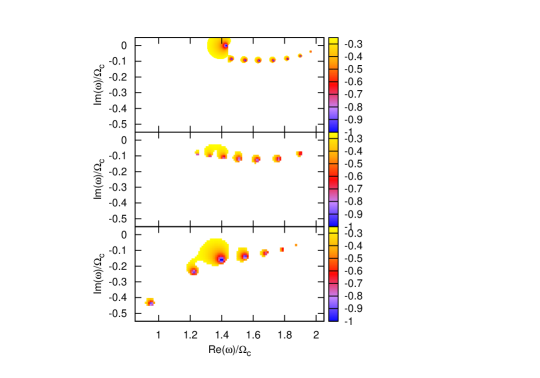
Figure 6: Heat map showing the position of (Landau) modes in the complex frequency plane for the lowered Spitzer sheet with $W=2$ (top panel) and $W=5$ (middle panel) and for the isothermal plane (bottom panel). Colors indicate log-base 10 of the eigenvalue of the matrix $M_{ij}-\delta_{ij}$ that comes closest to zero.

Figure 7: Positions of solutions to the dispersion equation for the $W=2$ lowered Spitzer plane. The cluster of modes at ${\rm Re}(\omega)/\Omega_{c}\simeq 1.7$ and ${\rm Im}(\omega)/\Omega_{c}\simeq-0.07$ is the same as the modes depicted in the top panel of Figure 6.

4 SIMULATIONS

In this section, we present results from a simple one-dimensional simulation that illustrates the behaviour predicted by our linear theory calculations. Our N-body system comprises self-gravitating, collisionless infinite sheets. We use a particle-mesh scheme in which the density is calculated on a one-dimensional grid and the force on a sheet at position $z$ is determined from the integral

$$F(z)=2\pi G\int dz^{\prime}\,\rho(z^{\prime}){\rm sgn}\left(z^{\prime}-z\right)~{}.$$ (47)

Similar simulations were presented in Weinberg (1991); Widrow et al. (2012) and Widrow et al. (2014).

We use initial conditions that correspond to a simple breathing mode by first setting up an equlibrium distribution and then perturbing the positions and velocities according to the relations $z=\lambda_{z}z_{e}$ and $v=\lambda_{v}v_{e}$ where ($z_{e},\,v_{e}$) are the phase space coordinates of a particle in the unperturbed system and $\lambda_{e,v}$ are constants. With our choice of units, the total kinetic and potential energies of the unperturbed system are $T=1/2\pi$ and $V=1/\pi$ respectively. With this in mind, we choose $\lambda_{v}=\left(3-2\lambda_{z}\right)^{1/2}$. The total energy of the perturbed and unperturbed systems are therefore the same while the initial virial ratio for the perturbed system is $R=2T/V=\left(3-2\lambda_{z}\right)/\lambda_{z}$.

In Figure 8 we show the time evolution of various system properties for a simulation with $200K$ particles and $\lambda_{z}=0.9$. For example, in the upper left panel, we show the virial ratio $R$. During the initial phase from $t=0$ to $t\simeq 12$ the amplitude of the oscillations in $R$ damps from an initial value of $0.3$ to $\sim 0.02$. The time-dependence of $R$ during this phase can be described by a model comprised of the sum of damped exponentials:

$$R=R_{0}+\sum_{i=1}^{n}C_{i}\cos{\left(\omega_{i}t-\beta_{i}\right)}e^{-\alpha_{i}t}~{}.$$ (48)

The fit for the run shown in Figure 8 has two terms with $\left(\omega_{i},\,\alpha_{i}\right)\simeq\left(1.5,\,0.25\right),\,\left(2.0,\,0.24\right)$. Note that we only fit Eq. 48 for $t<12$. At later times, perturbations are driven by the Poisson noise of the simulation (see below). The simulation results are in good qualitative agreement with our analytic results. In particular, the lower panel of Figure 6 shows that the typical modes of the Spitzer sheet have an oscillation frequency of ${\rm Re}(\omega)\simeq 2$ and an exponential damping constant of ${\rm Im}(\omega)\simeq 0.2$. However, because the oscillations damp after only a few cycles we are unable to resolve the detailed mode structure anticipated in Figure  6.

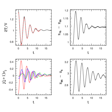
Figure 8: Time evolution of a perturbed plane symmetric collisionless system. The upper left panel shows the virial ratio $R\equiv 2T/V$ as a function of time (black solid curve) as well as a two-term fit based on Eq. 48 (red dashed curved). The lower left panel shows the first four even coefficients $j\left(j+1\right)c_{j}$ that appear in the expansion for the density. Colors are red, blue, magenta, and green for $j=2,\,4,\,6$ and $8$ respectively. The upper right panel shows the time evolution of the width of the region that contains the inner $50\%$ of the mass. The lower right panel shows the same for the inner $90\%$ of the mass.

A key feature of vertical oscilations is that they damp most rapidly in the inner parts of the distribution. This is illustrated in the lower left panel of Figure 8 where we see that the damping rate decreases with increasing $j$. Furthermore, if we compare the top and bottom panels on the right, we see that the oscillations of the region containing 50% of the mass damp more rapidly than the oscilations of the region containing 90% of the mass. Widrow et al. (2014) also noticed that the high energy part of the distribution function was more susceptible to vertical oscillations that were provoked by a passing satellite. We can therefore predict that bulk vertical motions will be strongest among stars in the high (vertical) energy tail of the phase space distribution.

At late times, the initial perturbation has damped away but oscilations, seeded by Poisson noise due to the finite number of particles, persist. In Figure 9 we show late time behaviour of a low-resolution (10K particle) simulation that was evolved until $t\simeq 1300$. We show a portion of the time evolution of the virial ratio (upper panel) and the power spectrum of the time-domain Fourier transform (lower panel). We see that there are continous oscillations with randomly changing phase and amplitude but with a characteristic frequencies of $\omega\simeq 2$ and $\omega\simeq 4$.

Figure 9: Results from a low resolution simulation with 10K particles that was run until $t=1300$. The upper panel shows a small section of the time evolution of the virial ratio while the lower panel shows the power spectrum.

5 DISCUSSION AND CONCLUSIONS

A passing satellite can irrevocably change the properties of a galactic disk in two fundamental ways. First, orbital energy from the satellite can be transferred to disk stars thereby heating and thickening the disk. Second, the satellite can provoke the formation of secular phenomena such as a bar, warp, or spiral structure. In either case, the initial response of the disk to the satellite can involve coherent oscillations. The subsequent evolution of these motions is governed by a mix of processes that include the restoring force of the disk’s own self-gravity, Landau damping, differential rotation, and swing amplification of spiral waves. In this paper, we have focused on the first two of these effects by restricting our attention to plane symmetric systems. Indeed, the structure of the oscillatory behaviour for a self-gravitating, plane-symmetric system is already quite complicated, especially in the case of a collisionless (i.e., stellar) system. There, the modes form a double series defined by two eigenvalues, one that determines the mode’s frequency and the other that determines its spatial structure

Linear perturbations of both gaseous and stellar plane symmetric systems divide neatly according to their parity with respect to the Galactic midplane. The North-South asymmetries in the number counts found in Widrow et al. (2012) and Yanny & Gardner (2013) by construction picked out odd parity density modes. Bending modes, which correspond local displacements of the disk from the midplane, can also be thought of as odd parity density perturbations. The midplane displacements seen in the interstellar medium (Nakanishi & Sofue, 2006) are an example of this.

By contrast modes where the density perturbation has even parity have bulk velocity fields that are odd in parity. The simplest example is the breathing mode perturbation, which may be present in the SEGUE (Widrow et al., 2012), RAVE (Williams et al., 2013), and LAMOST (Carlin et al., 2013) data sets. Unfortunately, a clear picture of the velocity field throughout the 1-2 kiloparsec neighbourhood of the Sun is lacking in large part because of the complicated and incomplete footprints of the surveys (see Carlin et al. (2013) for a detailed discussion). A combined analysis of the three data sets might improve this situation as will satellite data from Gaia (Perryman et al., 2001). As well, Bovy et al. (2014) proposed an alternative way to characterize the velocity field of the Galactic disk. The idea is to calculate the power spectrum of the velocity field after subtracting an axisymmetric model that accounts for the rotation of the disk. They find that the largest contribution to the power spectrum on large scales comes from the Sun’s motion relative to the local standard of rest. In addition, they find a broad peak in the power spectrum with $0.2\,{\rm kpc}^{-1}<k<0.9\,{\rm kpc}^{-1}$ and the associated motions might be associated with the time-dependent gravitational potential of the bar. While their analysis uses only heliocentric line-of-sight velocities and focuses on the two-dimensional in-plane velocity field, the technique could easily be extended to include proper motions and velocities perpendicular to the Galactic plane.

Robin et al. (2003) estimate the density of stars and dark matter in the midplane of the Galaxy at the position of the Sun is $\rho_{c}\simeq 0.055\,M_{\odot}\,{\rm pc}^{-3}$. The period of vertical oscillations for a star near the midplane is therefore $T_{c}\simeq 110\,{\rm Myr}$ or approximately one half the period for a star at this radius to orbit about the center of the Galaxy. In Section 3, we found that in the solar neighbourhood, the ratio of the exponential decay time to the vertical oscillation period for pure vertical modes typically fell in the range $\tau/T\simeq 2.5-8$. Thus, these modes might be expected to persist for $1-4$ orbital periods or $200-800\,{\rm Myr}$.

Of course, any application of our results to the Milky Way will require a more detailed understanding of how vertical modes couple to modes in the disk plane. As a satellite galaxy passes through the disk, it excites both bending and breathing modes (Widrow et al., 2014). The former have been implicated in the generation of galactic warps. Debattista (2014) has shown that spiral arms generate compression and rarefaction in the disk but the reverse seems plausible, namely that the compression and rarefaction perturbations due to a satellite, sheared by differential rotation of the disk, generate spiral structure. Sellwood & Carlberg (2014) have argued that spiral activity in disk galaxies arise from the superposition of transient unstable spiral modes. Satellite galaxies and dark matter subhalos would seem to provide a natural seed for these instabilities.

Appendix A MATRIX ELEMENTS FOR THE FLUID CASE

In this appendix, we describe the calculation of the matrix elements $M_{jk}$ in Eq. 16. As indicated in the text, we multiply both sides of Eq. 10 by $-\psi_{j}$ and integrate with respect to $z$ from $-\infty$ to $\infty$. The left hand side becomes $\omega^{2}c_{j}$.

The first two terms on the right-hand side of Eq. 10 can be combined to give

$$\int_{-\infty}^{\infty} dz\,\psi_{j}\left(\frac{d^{2}\rho_{1}}{dz^{2}}+\frac{d\psi_{0}}{dz}\frac{d\rho_{1}}{dz}\right)$$ (49)

$$=\int_{-1}^{1}du\,\left(1-u^{2}\right)\psi_{j}\frac{d^{2}\rho_{1}}{du^{2}}$$ (50)

$$=\sum_{k}{\cal N}_{jk}\int_{-1}^{1}du\,\left(1-u^{2}\right)P_{j}\frac{d^{2}}{du^{2}}\left(\left(1-u^{2}\right)P_{k}\right)$$ (51)

where ${\cal N}_{jk}=k\left(k+1\right)N_{j}N_{k}$. We can then use Legendre’s differential equation as well as the identity

$$\left(1-u^{2}\right)P^{\prime}_{j}(u)=j\left(P_{j-1}(u)-uP_{j}\right)$$ (52)

to write this expression in terms of the integrals

$$I_{j_{k}}^{1}=\int_{-1}^{1}du\,P_{j}(u)P_{k}(u)~{},$$ (53)

$$I_{j_{k}}^{2}\equiv\int_{-1}^{1}du\,u^{2}P_{j}(u)P_{k}(u)$$ (54)

and

$$I_{j_{k}}^{3}\equiv\int_{-1}^{1}du\,uP_{j}(u)P_{k-1}(u)~{},$$ (55)

which can be evaluated analytically (Arfken & Weber, 2005; Weisstein, 2014).

The third and fifth terms of Eq. 10 can be combined to yield

$$\int_{-\infty}^{\infty}dz\,\psi_{j} \left(\rho_{1}\frac{d^{2}\psi_{0}}{dz^{2}}+\rho_{0}\frac{d^{2}\psi_{1}}{dz^{2}}\right)$$ (56)

$$=-4\sum_{k}{\cal N}_{jk}\left(I_{j_{k}}^{1}-I_{j_{k}}^{2}\right)$$ (57)

while the fourth term gives

$$\int_{-\infty}^{\infty}dz\,\psi_{j}\frac{d\rho_{0}}{dz}\frac{d\psi_{1}}{dz}{dz}=4\sum_{k}kN_{j}N_{k}\left(I^{2}_{jk}-I^{3}_{jk}\right)~{}.$$ (58)

Appendix B HOMOGENEOUS SLAB

For the lowest order even parity mode ($j=1$) the potential can be written as

$$\psi_{1}=\frac{3N_{1}}{2}\left(E\cos^{2}\theta-1\right)$$ (59)

while density is constant: $\rho_{1}=3N_{1}/4\pi$. Since we are considering an even parity mode, we can write the Fourier series for $\psi$ as

$$\psi_{1}=\sum_{n=0}^{\infty}\psi_{1,n}\cos{n\theta}~{}.$$ (60)

We note that the $n=0$ term does not contribute to the distribution function. The relevant Fourier coefficient is then $\psi_{1,2}=3N_{1}E/4$ distribution function is then

$${\rm Re}\left(f_{1}\right)=\frac{df_{0}}{dE}\frac{3N_{1}E}{2}\frac{\cos{2\theta}}{2-\omega^{2}/4}~{}.$$ (61)

In order to show that this is indeed a true mode of the system, we calculate the density directly from the distribution function: $\rho_{1}=\int dv\,f_{1}$. As discussed in the text, this integral formally diverges but can be handled by considering a family of equilibrium distribution functions $f_{\lambda}(E)$ that approximate $f_{0}$ but are continuous at $E=1$. We then have

$$\int dv\,v^{2}\frac{df_{\lambda}}{dE}=\int dv\,v\frac{df_{\lambda}}{dv}=-\int dv\,f_{\lambda}=-\rho_{0}$$ (62)

where at the last equality, we let $\lambda\to\infty$. Moreover, the term proportional to $z^{2}$ vanishes. To see this, write $df_{0}/dE=\left(1/2z\right)df_{0}/dz$ and perform the integration over velocities before differentiating. The net result is that

$$\rho_{1}=\frac{3N_{1}}{8\pi}\frac{1}{2-\omega^{2}/4}~{},$$ (63)

which gives $\omega=6^{1/2}$ (Antonov, 1971; Kalnajs, 1973; Fridman et al., 1984).

The next mode ($j=3$) is

$$\psi_{3}=N_{3}\left(P_{4}(z)-P_{2}(z)\right)=\frac{7N_{3}}{8}\left(5z^{2}-1\right)\left(z^{2}-1\right)~{}.$$ (64)

Writing out in terms of trig functions

$$\psi_{3}=\frac{7N_{3}}{8}\left(5E^{2}\cos^{4}\theta-6E\cos^{2}\theta+1\right)~{}.$$ (65)

With the help of various trigonometric identities, we find

$$\psi_{3,4}=\frac{7N_{3}}{8}\frac{5E^{2}}{8}$$ (66)

and

$$\psi_{3,2}=\frac{7N_{3}}{8}\left(\frac{5E^{2}}{2}-3E\right)~{}.$$ (67)

Thus, for the distribution function, we have

$$Re\left(f_{3}\right)=\frac{df_{0}}{dE}\left(\frac{2\psi_{3,2}}{2-\omega^{2}/4}\cos{2\theta}+\frac{2\psi_{3,4}}{2-\omega^{2}/16}\cos{4\theta}\right)~{}.$$ (68)

A straightforward, but tedious calculation similar to the one performed above leads to an expression for $\rho_{3}$, which, when combined with Eq. 65, yields a quadratic equation for $\omega^{2}$ whose solutions are $\omega/\Omega_{c}=2.07,\,3.83$.

Appendix C DYNAMICS IN THE COMPLEX ENERGY PLANE

For the Spitzer sheet, we can find the density as a function of the potential by integrating the distribution function (Eq. 43) over $v$:

$$\rho\left(\psi\right)=\int_{-\infty}^{\infty}dv\,f(E)=\frac{1}{2\pi}e^{-\psi}~{}.$$ (69)

The Poisson equation $d^{2}\psi/dz^{2}=2\exp{\left(-\psi\right)}$ can then be integrated to obtain as expression for the force as a function of the potential:

$$F\left(\psi\right)=-\frac{d\psi}{dz}=-2\left(1-e^{-\psi}\right)^{1/2}~{}.$$ (70)

The period for a particle with energy $E$ is

$$T(E) =-4\int_{v_{\rm max}}^{v(t)}\frac{dv^{\prime}}{F\left(\psi\right)}$$ (71)

$$=2^{3/2}E^{1/2}\int_{0}^{\pi/2}\frac{\cos{\varphi}d\varphi}{\left(1-e^{-E\cos^{2}\varphi}\right)^{1/2}}$$ (72)

where $v_{\rm max}$ is the maximum velocity of the particle along its orbit (Araki, 1985). In deriving the second expression, we write $v$ and $\psi$ in terms of the parameter $\varphi$:

$$v=\left(2E\right)^{1/2}\sin{\varphi}~{}~{}~{}~{}~{}~{}~{}\psi=E\cos^{2}{\varphi}$$ (73)

More generally, we can write $t$ along the first quarter of the particle’s orbit as a function of $\varphi$:

$$t\left(\varphi,\,E\right)=\left(\frac{E}{2}\right)^{1/2}\int_{0}^{\varphi(t)}\frac{\cos\varphi^{\prime}d\varphi^{\prime}}{\left(1-e^{-E\cos^{2}\varphi^{\prime}}\right)^{1/2}}$$ (74)

Similarly

$$z\left(\varphi,\,E\right)=E\int_{0}^{\varphi(t)}\frac{\sin{\varphi^{\prime}}\cos{\varphi^{\prime}}d\varphi^{\prime}}{\left(1-e^{-E\cos^{2}{\varphi}^{\prime}}\right)^{1/2}}$$ (75)

For the lowered Spitzer sheet, $\rho(\psi)$ is given by

$$\rho(\psi)=f_{W}e^{-\psi}\left(\left(2\pi\right)^{1/2}{\rm erf}\left(y\right)-2^{3/2}ye^{-y^{2}}\right)$$ (76)

where $y=\left(W-\psi\right)^{1/2}/\sigma$. As before, we integrate the Poisson equation and find

$$F(\psi)=\left(8\pi\right)^{1/2}\left({\cal F}\left(y_{0}\right)-{\cal F}\left(y\right)\right)^{1/2}$$ (77)

where $y_{0}\equiv W^{1/2}$ and

$${\cal F}(z)=\left(2\pi\right)^{1/2}e^{z^{2}}{\rm erf}z-2^{3/2}\left(z+\frac{2z^{3}}{3}\right)$$ (78)

Finally, we write the complex Fourier coefficients of the basis functions $\psi_{j}$ as

$$\psi_{nj}(E)=\frac{1}{T(E)}\int_{0}^{2\pi}d\varphi\,\frac{dt}{d\varphi}\,\psi_{j}\left(z\left(E,\,\theta\right)\right)e^{-in\theta}$$ (79)

where $z$, $t$, and $\theta$ are complex functions of $E$ and of the real integration variable $\varphi$ through Eqs. 74 and 75.

References

- Anderson et al. (1992) Anderson, E., Bai, Z., & Bischof, C. 1992, Philadelphia, PA: SIAM (Society for Industrial and Apllied Mathematics), 1992, For Release 1.0 of LAPACK, edited by Anderson, E.; Bai, Z.; Bischof, C.,
- Antonov (1971) Antonov, V. A. 1971, Trudy Astronomicheskoj Observatorii Leningrad, 28, 64
- Araki (1985) Araki, S. 1985, Ph.D. Thesis, Massachusetts Institute of Technology
- Arfken & Weber (2005) Arfken, G. B., & Weber, H. J. 2005, ”Mathematical methods for physicists 6th ed.by George B. Arfken and Hans J. Weber. Published :Amsterdam; Boston : Elsevier
- Binney & Tremaine (2008) Binney, J., & Tremaine, S. 2008, Galactic Dynamics: Second Edition, by James Binney and Scott Tremaine. ISBN 978-0-691-13026-2 (HB). Published by Princeton University Press, Princeton, NJ USA, 2008
- Benson et al. (2004) Benson, A. J., Lacey, C. G., Frenk, C. S., Baugh, C. M., & Cole, S. 2004, MNRAS, 351, 1215
- Bovy (2010) Bovy, J. 2010, ApJ, 725, 1676
- Bovy et al. (2014) Bovy, J., Bird, J. C., García Pérez, A. E., & Zasowski, G. 2014, arXiv:1410.8135
- Camm (1950) Camm, G. L. 1950, MNRAS, 110, 305
- Carlin et al. (2013) Carlin, J. L., DeLaunay, J., Newberg, H. J., et al. 2013, arXiv:1309.6314
- Chandrasekhar (1943) Chandrasekhar, S. 1943, ApJ, 97, 255
- Cui et al. (2012) Cui, X.-Q., Zhao, Y.-H., Chu, Y.-Q., et al. 2012, Research in Astronomy and Astrophysics, 12, 1197
- Debattista (2014) Debattista, V. P. 2014, MNRAS, 443, L1
- Dehnen (2000) Dehnen, W. 2000, AJ, 119, 800
- Deng et al. (2012) Deng, L.-C., Newberg, H. J., Liu, C., et al. 2012, Research in Astronomy and Astrophysics, 12, 735
- Dubinski et al. (2008) Dubinski, J., Gauthier, J.-R., Widrow, L., & Nickerson, S. 2008, Formation and Evolution of Galaxy Disks, 396, 321
- Faure et al. (2014) Faure, C., Siebert, A., & Famaey, B. 2014, MNRAS, 440, 2564
- Feldmann & Spolyar (2015) Feldmann, R., & Spolyar, D. 2015, MNRAS, 446, 1000
- Fridman et al. (1984) Fridman, A. M., Polyachenko, V. L., Aries, A. B., & Poliakoff, I. N. 1984, Physics of gravitating systems. I. Equilibrium and stability.. A. M. Fridman, V. L. Polyachenko, translated by A. B. Aries, I. N. Poliakoff.Springer Verlag, New York
- Fux (2001) Fux, R. 2001, A&A, 373, 511
- Gao et al. (2004) Gao, L., White, S. D. M., Jenkins, A., Stoehr, F., & Springel, V. 2004, MNRAS, 355, 819
- Gauthier et al. (2006) Gauthier, J.-R., Dubinski, J., & Widrow, L. M. 2006, ApJ, 653, 1180
- Gómez et al. (2012) Gómez, F. A., Minchev, I., Villalobos, Á., O’Shea, B. W., & Williams, M. E. K. 2012, MNRAS, 419, 2163
- Gómez et al. (2012) Gómez, F. A., Minchev, I., O’Shea, B. W., et al. 2012, MNRAS, 423, 3727
- Gómez et al. (2013) Gómez, F. A., Minchev, I., O’Shea, B. W., et al. 2013, MNRAS, 429, 159
- Huang & Carlberg (1997) Huang, S., & Carlberg, R. G. 1997, ApJ, 480, 503
- Hunter & Toomre (1969) Hunter, C., & Toomre, A. 1969, ApJ, 155, 747
- Kalnajs (1971) Kalnajs, A. J. 1971, ApJ, 166, 275
- Kalnajs (1973) Kalnajs, A. J. 1973, ApJ, 180, 1023 (erratum: 1973, ApJ, 185, 393)
- Kalnajs (1977) Kalnajs, A. J. 1977, ApJ, 212, 637
- Kazantzidis et al. (2008) Kazantzidis, S., Bullock, J. S., Zentner, A. R., Kravtsov, A. V., & Moustakas, L. A. 2008, ApJ, 688, 254
- Klypin et al. (1999) Klypin, A., Kravtsov, A. V., Valenzuela, O., & Prada, F. 1999, ApJ, 522, 82
- Kuijken & Gilmore (1989) Kuijken, K., & Gilmore, G. 1989, MNRAS, 239, 571
- Landau (1946) Landau, L., 1946, J. Phys. USSR 10 (JETP, 16, 574)
- Louis (1992) Louis, P. D. 1992, MNRAS, 258, 552
- Lynden-Bell (1962) Lynden-Bell, D. 1962, MNRAS, 124, 279
- Lynden-Bell (1965) Lynden-Bell, D. 1965, MNRAS, 129, 299
- Mathur (1990) Mathur, S. D. 1990, MNRAS, 243, 529
- Minchev et al. (2009) Minchev, I., Quillen, A. C., Williams, M., et al. 2009, MNRAS, 396, L56
- Moore et al. (1999) Moore, B., Ghigna, S., Governato, F., et al. 1999, ApJL, 524, L19
- Nakanishi & Sofue (2006) Nakanishi, H., & Sofue, Y. 2006, PASJ, 58, 847
- Oort (1932) Oort, J. H. 1932, BAN, 6, 249
- Perryman et al. (2001) Perryman, M. A. C., de Boer, K. S., Gilmore, G., et al. 2001, A&A, 369, 339
- Purcell et al. (2011) Purcell, C. W., Bullock, J. S., Tollerud, E. J., Rocha, M., & Chakrabarti, S. 2011, Nature, 477, 301
- Quinn et al. (1993) Quinn, P. J., Hernquist, L., & Fullagar, D. P. 1993, ApJ, 403, 74
- Robin et al. (2003) Robin, A. C., Reylé, C., Derrière, S., & Picaud, S. 2003, A&A, 409, 523
- Sellwood (2013) Sellwood, J. A. 2013, Planets, Stars and Stellar Systems. Volume 5: Galactic Structure and Stellar Populations, 923
- Sellwood et al. (1998) Sellwood, J. A., Nelson, R. W., & Tremaine, S. 1998, ApJ, 506, 590
- Sellwood & Carlberg (2014) Sellwood, J. A., & Carlberg, R. G. 2014, ApJ, 785, 137
- Spitzer (1942) Spitzer, L., Jr. 1942, ApJ, 95, 329
- Spitzer (1958) Spitzer, L., Jr. 1958, ApJ, 127, 17
- Steinmetz et al. (2006) Steinmetz, M., Zwitter, T., Siebert, A., et al. 2006, AJ, 132, 1645
- Toth & Ostriker (1992) Toth, G., & Ostriker, J. P. 1992, ApJ, 389, 5
- Toomre (1966) Toomre, A. 1966, in Geophys. Fluid Dyn. (Notes on the 1966 Summer Study Program at the Woods Hole Oceanographic Institute, Ref. No. 66-46) 66 J. 1972, ApJ, 178, 623
- Walker et al. (1996) Walker, I. R., Mihos, J. C., & Hernquist, L. 1996, ApJ, 460, 121
- Walters & Cox (2001) Walters, M. A., & Cox, D. P. 2001, ApJ, 549, 353
- Weinberg (1991) Weinberg, M. D. 1991, ApJ, 373, 391
- Weisstein (2014) Weisstein, Eric W. “Legendre Polynomial.” From MathWorld–A Wolfram Web Resource. http://mathworld.wolfram.com/LegendrePolynomial.html
- Widrow et al. (2012) Widrow, L. M., Gardner, S., Yanny, B., Dodelson, S., & Chen, H.-Y. 2012, ApJL, 750, L41
- Widrow et al. (2014) Widrow, L. M., Barber, J., Chequers, M. H., & Cheng, E. 2014, MNRAS, 440, 1971
- Williams et al. (2013) Williams, M. E. K., Steinmetz, M., Binney, J., et al. 2013, arXiv:1302.2468
- Yanny & Gardner (2013) Yanny, B., & Gardner, S. 2013, arXiv:1309.2300
- Yanny et al. (2009) Yanny, B., Rockosi, C., Newberg, H. J., et al. 2009, AJ, 137, 4377
- Zhao et al. (2012) Zhao, G., Zhao, Y.-H., Chu, Y.-Q., Jing, Y.-P., & Deng, L.-C. 2012, Research in Astronomy and Astrophysics, 12, 723